


ABSTRACT
We report on the results of four XMM–Newton observations separated by about ten days from each other of Cyg OB2 #8A [O6If + O5.5III(f)]. This massive colliding wind binary is a very bright X-ray emitter — one of the first X-ray emitting O-stars discovered by the Einstein satellite — as well as a confirmed non-thermal radio emitter whose binarity was discovered quite recently. The X-ray spectrum between 0.5 and 10.0 keV is essentially thermal, and is best fitted with a three-component model with temperatures of about 3, 9 and 20 MK. The X-ray luminosity corrected for the interstellar absorption is rather large, i.e. about 1034 erg s−1. Compared to the ‘canonical’LX/Lbol ratio of O-type stars, Cyg OB2 #8A was a factor of 19–28 overluminous in X-rays during our observations. The EPIC spectra did not reveal any evidence for the presence of a non-thermal contribution in X-rays. This is not unexpected considering that the simultaneous detections of non-thermal radiation in the radio and soft X-ray (below 10.0 keV) domains is unlikely. Our data reveal a significant decrease in the X-ray flux from apastron to periastron with an amplitude of about 20 per cent. Combining our XMM–Newton results with those from previous ROSAT-PSPC and ASCA-SIS observations, we obtain a light curve suggesting a phase-locked X-ray variability. The maximum emission level occurs around phase 0.75, and the minimum is probably seen shortly after the periastron passage. Using hydrodynamic simulations of the wind–wind collision, we find a high X-ray emission level close to phase 0.75, and a minimum at periastron as well. The high X-ray luminosity, the strong phase-locked variability and the spectral shape of the X-ray emission of Cyg OB2 #8A revealed by our investigation point undoubtedly to X-ray emission dominated by colliding winds.
1 INTRODUCTION
The Cyg OB2 (VI Cygni) association has several particularities that stimulated the interest of astronomers. It has a diameter of about 2°, corresponding to about 60 pc at a distance of 1.7 kpc (Knödlseder 2000). It harbours a huge number of early-type stars: about 100 O-type and probably more than 2000 B-type stars (Knödlseder 2000; Comerón et al. 2002). Considering its mass, density and size, Knödlseder (2000) proposed it may be the first object in the Galaxy to be reclassified as a young globular cluster. However, a complete census of the massive star content of Cyg OB2 is not easy to achieve because of the heavy extinction in this direction (Comerón et al. 2002). So far, a spectral classification has only been proposed for its brightest and bluest members (Massey & Thompson 1991).
Another particularity of Cyg OB2 is that it contains some of the brightest OB stars of our Galaxy (see e.g. Herrero, Puls & Najarro 2002), among which we find some of the brightest X-ray emitting early-type stars. Historically, the Einstein X-ray observatory discovered the first X-ray sources whose optical counterparts were known to be massive stars in Cyg OB2, i.e. Cyg OB2 #5, #8A, #9 and #12 (Harnden et al. 1979). The same field was further investigated with various X-ray observatories: ROSAT (Waldron et al. 1998), ASCA (Kitamoto & Mukai 1996; De Becker 2001) and more recently Chandra (Waldron et al. 2004). This paper is the first of a series presenting the XMM–Newton view of Cyg OB2. It will focus on its brightest X-ray emitter, i.e. Cyg OB2 #8A (BD +40° 4227).
Cyg OB2 #8A was recently discovered to be a binary system consisting of an O6If primary and an O5.5III(f) secondary (De Becker, Rauw & Manfroid 2004c; De Becker & Rauw 2006). The system is eccentric (e= 0.24 ± 0.04) with a period of 21.908 ± 0.040 d and a major axis of 142 ± 6 R⊙. The fact that Cyg OB2 #8A is a binary system could reconcile the high bolometric luminosity reported by Herrero et al. (2002) with its spectral classification, believed at that time to be a single O5.5I(f) star. The analysis of a time-series of the He ii λ 4686 line revealed a phase-locked profile variability likely attributed to a wind–wind interaction (De Becker & Rauw 2006).
In the framework of the campaign devoted to the multiwavelength study of non-thermal radio emitters (see De Becker 2005), Cyg OB2 #8A is a particularly interesting target. The non-thermal radio emission, supposed to be synchrotron radiation (White 1985), requires (i) the presence of a magnetic field and (ii) the existence of a population of relativistic electrons. Although in the past few years the first direct measurements of surface magnetic fields have been performed for a few early-type stars, e.g. β Cep (Donati et al. 2001), θ1 Ori C (Donati et al. 2002) and ζ Cas (Neiner et al. 2003), the estimation of the strength of the magnetic field of massive stars remains a difficult task. Indeed, the Zeeman effect in spectral lines is concealed by the large rotational broadening of massive stars. Therefore, our knowledge of magnetic fields in early-type stars is at most fragmentary. The relativistic electrons are supposed to be accelerated through the first-order Fermi mechanism described for instance by Bell (1978), and applied to the case of massive stars by Pollock (1987), Eichler & Usov (1993) and Chen & White (1994). This process requires the presence of hydrodynamic shocks. We mention that an alternative scenario was proposed by Jardine, Allen & Pollock (1996), but we will assume here that the first-order Fermi mechanism in the presence of hydrodynamic shocks (the so-called diffusive shock acceleration–DSA–mechanism) is the dominant process. For a discussion of the physical processes involved in the general scenario of the non-thermal emission from massive stars, we refer, for example, to De Becker, Rauw & Swings (2005a) and references therein. The issue to be addressed here is that of the nature of these shocks: are they intrinsic to the stellar winds (see e.g. Feldmeier, Puls & Pauldrach 1997), or are they due to the wind–wind collision in a binary system (see e.g. Stevens, Blondin & Pollock 1992).
In the case of Wolf–Rayet (WR) stars, the non-thermal radio emitters are mostly binary systems: out of 17, 14 are at least suspected binaries (for a general discussion, see De Becker 2005). In some cases the non-thermal emitting region has been resolved and is clearly associated with the colliding-wind region (see e.g. the case of WR 140 Dougherty et al. 2005). But for the O-stars, the situation is less clear even though the fraction of binaries (confirmed or suspected) among non-thermal radio emitters has recently evolved to a value closer to that of WR stars. We know indeed that among the 16 non-thermal O-type radio emitters, 11 are confirmed binaries and two more are suspected binaries (see De Becker 2005). The recent discovery of the binarity of Cyg OB2 #8A lends further support to the second scenario where the population of relativistic electrons, and consequently the non-thermal radio emission, is produced in the interaction zone between the winds of two stars (in this binary system).
In addition, one can wonder whether non-thermal radiation can be produced in the high-energy domain as a counterpart to this non-thermal emission in the radio waveband. The detection of radio synchrotron radiation is an evidence for the presence of relativistic electrons. The existence of such high-energy electrons suggests that other non-thermal emission mechanisms such as inverse Compton (IC) scattering may be at work. The relativistic electrons accelerated at the collision zone may transfer energy to the ultraviolet (UV) photons emitted by the photosphere of the stars, therefore upscattering them to the high-energy domain. As a result, these radio non-thermal emitting binary systems could be non-thermal emitters in the X-ray and soft γ-ray domains as well. In this context, several targets have been investigated in the X-ray domain with XMM–Newton: 9 Sgr (Rauw et al. 2002), HD 168112 (De Becker et al. 2004b) and HD 167971 (De Becker et al. 2005b). Up to now, no unambiguous detection of non-thermal X-ray emission has been revealed by the X-ray observations of non-thermal radio emitters.
Beside the putative non-thermal emission, the X-ray spectrum of massive binaries like Cyg OB2 #8A is expected to be dominated by thermal emission produced by the plasma heated by hydrodynamic shocks due to intrinsic instabilities or to the wind–wind collision. As a colliding wind binary, Cyg OB2 #8A might be compared to other massive binaries where the colliding winds contribute significantly to the thermal X-ray emission (see for instance WR 140, Pollock et al. 2005; and WR 25, Pollock & Corcoran 2005). In this context, the possibility to detect a non-thermal emission component as discussed above will depend strongly on the properties of the thermal emission contributions. De Becker et al. (2005b) discussed the unlikelihood of the simultaneous detection of non-thermal radio and soft X-ray emission and proposed that short period binaries (a few days) were more likely to present a non-thermal X-ray emission below 10.0 keV than wide binaries. A more detailed discussion of this issue can be found in De Becker (2005). To investigate the X-ray emission of the massive members of Cyg OB2, we obtained four pointings with the XMM–Newton X-ray observatory. This paper is devoted to the massive binary Cyg OB2 #8A. The study of the other bright X-ray emitting massive stars, along with that of other fainter sources of the field, is postponed to a forthcoming paper.
The present paper is organized as follows. Section 2 describes the observations and the data reduction procedure. The spectral analysis of EPIC and RGS data of Cyg OB2 #8A is discussed in Section 3, whilst Section 4 is devoted to a discussion of the X-ray luminosity and to its variability. The discussion of archive X-ray data is provided in Section 5. Section 6 is devoted to a general discussion. Finally, Section 7 summarizes the main results of this analysis and presents the conclusions.
2 OBSERVATIONS
We have obtained four observations of Cyg OB2 with the XMM–Newton satellite, with a separation of about ten days between each pointing (see Table 1). The aim-point was set to the position of Cyg OB2 #8A in order to obtain high-resolution RGS spectra of this system. Because of the brightness of the massive stars located in the field of view we used the EPIC medium filter to reject optical light.
Observations of Cyg OB2 performed in 2004 with XMM–Newton. The columns yield, respectively, the (1) revolution number, (2) the observation ID, (3) the observation date, (4) the beginning and ending times expressed in Julian days, (5) the orbital phase at mid-exposure according to the ephemeris determined by De Becker et al. (2004c), and finally (6) the performed exposure time expressed in ks.
| Revolution number | Observation ID | Date | JD −2 453 300 | φ | Exposure time (ks) |
|---|---|---|---|---|---|
| (1) | (2) | (3) | (4) | (5) | (6) |
| 896 | 0200450201 | 10/29–30 | 8.458–8.701 | 0.534 | 21 |
| 901 | 0200450301 | 11/08–09 | 18.425–18.691 | 0.989 | 23 |
| 906 | 0200450401 | 11/18–19 | 28.399–28.688 | 0.445 | 25 |
| 911 | 0200450501 | 11/28–29 | 38.372–38.639 | 0.900 | 23 |
2.1 EPIC data
2.1.1 Data reduction
All three EPIC instruments were operated in the full frame mode (Turner et al. 2001; Strüder et al. 2001). We used the version 6.0.0 of the XMM Science Analysis System (sas) for the data reduction. The raw EPIC data of the four pointings were processed through the emproc and epproc tasks. The event lists were screened in the standard way: we considered only events with pattern 0–12 and pattern 0–4, respectively, for EPIC-MOS and EPIC-pn.
We selected the source X-ray events from inside a 60 arcsec radius circular region centred on Cyg OB2 #8A, excluding its intersection with a circular 15 arcsec radius region centred on Cyg OB2 #8C [right ascension (RA) = 20:33:17.9 and declination (Dec.) =+41:18:29.5, Equinox 2000.0]. The background region was defined as an annulus centred on the source and covering the same area as the circular source region, excluding its intersection with a 15 arcsec circular region centred on a point source (RA = 20:33:13.9 and Dec. =+41:20:21.4, Equinox 2000.0). For EPIC-MOS2 data, we excluded the intersection of these two regions (source and background) with a rectangular box to reject a bad column that crosses the central CCD, at slightly more than 30 arcsec away from the centre of the source region. We did the same in the case of EPIC-pn data to avoid a CCD gap located at about 40 arcsec from Cyg OB2 #8A. In each case, the boxes were adjusted after a careful inspection of the relevant exposure maps. Fig. 1 shows the source and background regions used for the three EPIC instruments in the case of Observation 1. The regions for the other observations differ only by the rotation angle. We generated the response matrix files (RMFs) with the rmfgen task for EPIC-MOS data. For EPIC-pn data, because of a problem with rmfgen,1 we used the canned response matrix for on-axis sources provided by the SOC. The ancilliary response files (ARFs) were generated with the arfgen task. We finally rebinned our spectra to get at least nine and 16 counts per energy bin, respectively, for EPIC-MOS and EPIC-pn. All our spectra were then analysed using the xspec software (see Section 3.1).

Source (circle) and background (annulus) regions selected for the spectrum extraction of Cyg OB2 #8A for the first XMM–Newton observation. Boxes were used to exclude the CCD gap for EPIC-pn and the bad column for EPIC-MOS2. Small circular regions were used to exclude faint point sources close to Cyg OB2 #8A. The EPIC-pn image was corrected for out of time (OOT) events. The inner circle has a radius of 60 arcsec. North is up and east is to the left-hand side.
2.1.2 High-level background episodes
We extracted a high-energy light curve (pulse invariant–PI–channel numbers >1000, i.e. photon energies above ∼10 keV) from the complete event lists to investigate the behaviour of the background level during the four pointings. High background time intervals are known to occur because of solar soft proton flares (Lumb 2002). We detected high background level episodes mostly in the fourth pointing. Even though such a high background level is not expected to affect significantly the spectral analysis of sources as bright as Cyg OB2 #8A (see e.g. De Becker et al. 2004a,b), we decided to filter our data sets to reject the most affected time intervals. After inspection of the light curves from the four data sets, we selected the time intervals below a threshold of 20 cts s−1 for EPIC-MOS and 75 cts s−1 for EPIC-pn. As a consequence, the effective exposure times are reduced (see Table 2) compared to the values provided in Table 1. However, this allows us to obtain the cleanest possible spectra thereby increasing the reliability of our analysis. As can be seen from the spectra shown for instance by De Becker et al. (2004b), the background correction produces spectra with large error bars on the normalized flux for spectral bins strongly affected by a high background level. In the case of bright sources like Cyg OB2 #8A, the data analysis does not suffer critically from the rejection of a fraction of the exposure time.
Effective exposure time of the Cyg OB2 observations after rejection of the flare contaminated time intervals.
| Observation 1 (ks) | Observation 2 (ks) | Observation 3 (ks) | Observation 4 (ks) | |
|---|---|---|---|---|
| EPIC-MOS1 | 18.6 | 20.9 | 22.9 | 12.6 |
| EPIC-MOS2 | 18.2 | 20.3 | 22.6 | 12.9 |
| EPIC-pn | 14.9 | 15.2 | 19.0 | 9.0 |
| RGS1 | 18.0 | 19.7 | 20.1 | 12.2 |
| RGS2 | 17.9 | 19.1 | 19.8 | 12.2 |
2.1.3 Pile-up?
Considering the X-ray brightness of Cyg OB2 #8A, one can wonder whether the EPIC data are affected by pile-up. According to the XMM–Newton User's Handbook, the count rate threshold above which pile-up may occur for point sources in full frame mode are about 0.7 and 8.0 cts s−1, respectively, for EPIC-MOS and EPIC-pn in full frame mode. As will be shown later (see Table 7), the critical value is reached for some EPIC-MOS data sets, and we have to check whether our data are affected.
First, we generated pattern histograms and searched for the presence of patterns 26–29 events expected to be due to pile-up. We did not find such patterns for any of our data sets. Next, we used the epatplot task to draw curves of the singlet and doublet events as a function of PI. We obtained a first series of curves on the basis of event lists filtered using the standard screening criteria and the spatial filter described here above for the source region. A second series of curves was then built on the basis of event lists obtained with a slightly modified spatial filter, where the core of the point spread function (PSF) was excluded. Since pile-up is expected to occur mainly in the core of the PSF, these latter event lists should essentially be unaffected. As the curves built using epatplot are supposed to be pile-up sensitive, we may expect some differences between the two sets of curves if our data are indeed affected. However, no significant differences were found. Consequently, we consider that our data are unaffected by pile-up.
2.2 RGS data
2.2.1 Data reduction
The two RGS instruments were operated in spectroscopy mode during the four observations (den Herder et al. 2001). The raw data were processed with the sas version 6.0.0 through the rgsproc task. The first and second-order spectra of the source were extracted using the rgsspectrum task. We selected the background events from a region spatially offset from the source region. The response matrices were constructed through the rgsrmfgen task for RGS1 and RGS2 data of the four pointings.
2.2.2 High background level episodes
We followed the same procedure as described in Section 2.1.2 to select good time intervals (GTIs) unaffected by soft proton flares. However, as the mean level of the light curves was different according to the data set and also to the instrument, we refrained from adopting the same count rate threshold for all the data. After rejection of the time intervals contaminated by the high background, we obtained the effective exposure times quoted in Table 2. As for the EPIC data, the pointing whose exposure time is the most severely reduced is the fourth one.
3 ANALYSIS OF CYG OB2 #8A DATA
3.1 Spectral analysis
As briefly discussed in Section 1, several physical mechanisms are expected to be responsible for the X-ray emission of massive stars. On the one hand, the heating of the plasma of the stellar winds by hydrodynamic shocks is responsible for a thermal emission. These shocks may occur in stellar winds of individual stars (see e.g. Feldmeier et al. 1997) or in the wind–wind collision zone of binary systems (see e.g. Stevens et al. 1992). These two types of hydrodynamic shocks are able to produce plasma with characteristic temperatures of the order of a few 106 K and of a few 107 K, respectively. To a first approximation, such a thermal emission can be modelled by optically thin thermal plasma models (mekal model: Mewe, Gronenschild & van den Oord 1985; Kaastra 1992). On the other hand, non-thermal emission processes like IC scattering are expected to produce a power-law component in the X-ray spectrum. In this section, we will use composite models made of mekal and power-law models. We note that solar abundances (Anders & Grevesse 1989) are assumed for the plasma throughout this paper.
3.2 Interstellar material and wind absorption
Absorption models are required to account for the fact that both local circumstellar (wind) and interstellar material (ISM) are likely to absorb a significant fraction of the X-rays. The ISM absorption column was fixed to a value of NH= 0.94 × 1022 cm−2 obtained from the dust-to-gas ratio given by Bohlin, Savage & Drake (1978), using the colour excess [E(B−V) = 1.6] provided by Torres-Dodgen, Tapia & Carroll (1991).
To account for the fact that the wind material is ionized, an ionized wind absorption model was used for the local absorption component. We adopted the same opacity table as in the case of the multiple system HD 167971 (De Becker et al. 2005b), obtained with the wind absorption model described by Nazé et al. (2004). Briefly, this model considers the absorption by the 10 most abundant elements (H, He, C, N, O, Ne, Mg, Si, S and Fe) fixed at their solar abundances. The stellar fluxes were taken from the Kurucz library of spectra. For details on the model, we refer to Nazé et al. (2004). In De Becker et al. (2005b), we showed that there were no significant differences between opacities derived from various sets of parameters covering at least spectral types from O5 to O8. From the optical data already presented in De Becker et al. (2004c), we can estimate some crucial stellar and wind parameters of the stars in Cyg OB2 #8A. Following the spectral types of the two components, i.e. O6If and O5.5III(f), we adopted typical stellar radii and effective temperatures from Martins, Schaerer & Hillier (2005), allowing us to estimate the bolometric luminosity of the two stars. The mass loss rates and terminal wind velocities were then obtained from the mass loss recipes of Vink, de Koter & Lamers (2000, 2001). These parameters are quoted in Table 3. Provided that the stellar parameters of Cyg OB2 #8A lie within the parameter space discussed by De Becker et al. (2005b), we estimated that the wind absorption model that we used for HD 167971 suits the local absorption of Cyg OB2 #8A as well.
Parameters of the two components of Cyg OB2 #8A mainly estimated on the basis of a comparison with typical values provided by Martins et al. (2005).
| Primary | Secondary | |
|---|---|---|
| Spectral type | O6If | O5.5III(f) |
| Teff (K) | 36 800 | 39 200 |
| R★ (R⊙) | 20.0 | 14.8 |
| M★ (M⊙) | 44.1 | 37.4 |
| Lbol (erg s−1) | 2.5 × 1039 | 1.8 × 1039 |
| log g | 3.48 | 3.67 |
 (M⊙ yr−1) (M⊙ yr−1) | 4.8 × 10⁻⁶ | 3.0 × 10⁻⁶ |
| V∞ (km s−1)a | 1873 | 2107 |
| Primary | Secondary | |
|---|---|---|
| Spectral type | O6If | O5.5III(f) |
| Teff (K) | 36 800 | 39 200 |
| R★ (R⊙) | 20.0 | 14.8 |
| M★ (M⊙) | 44.1 | 37.4 |
| Lbol (erg s−1) | 2.5 × 1039 | 1.8 × 1039 |
| log g | 3.48 | 3.67 |
| (M⊙ yr−1) | 4.8 × 10⁻⁶ | 3.0 × 10⁻⁶ |
| V∞ (km s−1)a | 1873 | 2107 |
The terminal velocities of both stars were estimated to be 2.6 times the escape velocities of the stars (Vink et al. 2000, 2001), calculated on the basis of the typical stellar values given by Martins et al. (2005).
Parameters of the two components of Cyg OB2 #8A mainly estimated on the basis of a comparison with typical values provided by Martins et al. (2005).
| Primary | Secondary | |
|---|---|---|
| Spectral type | O6If | O5.5III(f) |
| Teff (K) | 36 800 | 39 200 |
| R★ (R⊙) | 20.0 | 14.8 |
| M★ (M⊙) | 44.1 | 37.4 |
| Lbol (erg s−1) | 2.5 × 1039 | 1.8 × 1039 |
| log g | 3.48 | 3.67 |
| (M⊙ yr−1) | 4.8 × 10⁻⁶ | 3.0 × 10⁻⁶ |
| V∞ (km s−1)a | 1873 | 2107 |
The terminal velocities of both stars were estimated to be 2.6 times the escape velocities of the stars (Vink et al. 2000, 2001), calculated on the basis of the typical stellar values given by Martins et al. (2005).
3.3 EPIC spectra
In order to fit the EPIC spectra, we tried different models including mekal and power-law components. The quality of the fits was estimated using the χ2 minimization technique and the best-fitting parameter values are quoted in Table 4. We checked the consistency of our results with both the Cash statistic (Cash 1979) and the χ2 statistic using a Churazov weighting (Churazov et al. 1996). We did not find any significant differences in the results obtained with the three methods. This was not unexpected as we are dealing with good quality spectra containing rather large numbers of counts per energy bin.
Parameters for EPIC spectra of Cyg OB2 #8A in the case of a wabsISM*wind*(mekal1+mekal2+mekal3) model. Results are given for MOS1, pn and combined MOS1 plus pn (‘EPIC’) in the case of the four observations. The first absorption component (absISM) is frozen at the ISM value: 0.94 × 1022 cm−2. The second absorption column, quoted as Nw (in cm−2), stands for the absorption by the ionized wind material. The normalization parameter (Norm) of the mekal components is defined as  , where D, ne and nH are, respectively, the distance to the source (in cm), and the electron and hydrogen number densities (in cm−3). The indicated range in the parameter values represents the 90 per cent confidence interval. The last two columns give, respectively, the observed flux and the flux corrected for the ISM absorption between 0.5 and 10.0 keV.
| log Nw | kT1 (keV) | Norm1 (10−2) | kT2 (keV) | Norm2 (10−3) | kT3 (keV) | Norm3 (10−3) | χ2ν (d.o.f.) | Observed flux (erg cm−2 s−1) | Corrected flux (erg cm−2 s−1) | |
|---|---|---|---|---|---|---|---|---|---|---|
| Observation 1 | ||||||||||
| MOS1 | 21.7421.8221.67 | 0.230.270.20 | 4.9410.352.57 | 1.031.100.87 | 9.6712.215.95 | 1.982.601.66 | 4.938.262.72 | 1.26 (281) | 6.23 × 10⁻¹² | 3.36 × 10⁻¹¹ |
| pn | 21.6821.7321.62 | 0.260.290.23 | 2.664.101.68 | 0.790.830.76 | 9.8710.838.97 | 1.841.911.77 | 7.598.167.06 | 1.24 (636) | 6.85 × 10⁻¹² | 3.07 × 10⁻¹¹ |
| EPIC | 21.7021.7421.66 | 0.250.280.23 | 3.234.402.24 | 0.830.870.79 | 8.819.588.06 | 1.811.871.75 | 7.518.057.04 | 1.39 (924) | 6.61 × 10⁻¹² | 3.09 × 10⁻¹¹ |
| Observation 2 | ||||||||||
| MOS1 | 21.9622.0121.90 | 0.230.270.20 | 9.0017.884.05 | 0.820.970.75 | 10.1112.008.37 | 1.671.901.53 | 5.446.764.07 | 1.01 (265) | 4.87 × 10⁻¹² | 2.71 × 10⁻¹¹ |
| pn | 21.9021.9321.86 | 0.240.280.23 | 6.168.903.67 | 0.790.850.74 | 9.7410.928.56 | 1.571.661.50 | 6.607.465.70 | 1.05 (580) | 5.22 × 10⁻¹² | 2.64 × 10⁻¹¹ |
| EPIC | 21.9121.9521.89 | 0.240.260.22 | 6.559.664.53 | 0.800.850.75 | 9.7610.778.77 | 1.601.681.53 | 6.246.965.49 | 1.12 (852) | 5.15 × 10⁻¹² | 2.64 × 10⁻¹¹ |
| Observation 3 | ||||||||||
| MOS1 | 21.8021.8521.72 | 0.270.290.23 | 3.676.082.20 | 0.890.980.82 | 7.718.866.60 | 1.922.201.80 | 6.206.904.44 | 1.37 (296) | 5.85 × 10⁻¹² | 2.53 × 10⁻¹¹ |
| pn | 21.7021.7521.66 | 0.280.300.26 | 2.553.431.94 | 0.810.850.78 | 9.3410.148.60 | 1.911.981.85 | 7.187.596.74 | 1.21 (686) | 6.75 × 10⁻¹² | 2.88 × 10⁻¹¹ |
| EPIC | 21.7221.7921.69 | 0.280.300.26 | 2.714.412.10 | 0.830.870.79 | 8.759.488.01 | 1.921.981.86 | 6.847.226.41 | 1.49 (989) | 6.47 × 10⁻¹² | 2.76 × 10⁻¹¹ |
| Observation 4 | ||||||||||
| MOS1 | 21.9622.0121.89 | 0.220.240.19 | 14.9427.738.27 | 0.881.000.78 | 10.3612.318.04 | 1.722.161.53 | 5.327.162.77 | 1.17 (225) | 5.38 × 10⁻¹² | 3.89 × 10⁻¹¹ |
| pn | 21.8621.8921.80 | 0.240.280.23 | 8.3810.894.31 | 0.870.920.81 | 11.7813.0010.21 | 1.821.921.69 | 5.446.524.84 | 1.33 (506) | 6.31 × 10⁻¹² | 3.74 × 10⁻¹¹ |
| EPIC | 21.8921.9221.85 | 0.230.250.22 | 9.9313.286.97 | 0.870.920.82 | 11.3812.3810.10 | 1.821.901.69 | 5.216.164.68 | 1.56 (738) | 5.91 × 10⁻¹² | 3.73 × 10⁻¹¹ |
Parameters for EPIC spectra of Cyg OB2 #8A in the case of a wabsISM*wind*(mekal1+mekal2+mekal3) model. Results are given for MOS1, pn and combined MOS1 plus pn (‘EPIC’) in the case of the four observations. The first absorption component (absISM) is frozen at the ISM value: 0.94 × 1022 cm−2. The second absorption column, quoted as Nw (in cm−2), stands for the absorption by the ionized wind material. The normalization parameter (Norm) of the mekal components is defined as , where D, ne and nH are, respectively, the distance to the source (in cm), and the electron and hydrogen number densities (in cm−3). The indicated range in the parameter values represents the 90 per cent confidence interval. The last two columns give, respectively, the observed flux and the flux corrected for the ISM absorption between 0.5 and 10.0 keV.
| log Nw | kT1 (keV) | Norm1 (10−2) | kT2 (keV) | Norm2 (10−3) | kT3 (keV) | Norm3 (10−3) | χ2ν (d.o.f.) | Observed flux (erg cm−2 s−1) | Corrected flux (erg cm−2 s−1) | |
|---|---|---|---|---|---|---|---|---|---|---|
| Observation 1 | ||||||||||
| MOS1 | 21.7421.8221.67 | 0.230.270.20 | 4.9410.352.57 | 1.031.100.87 | 9.6712.215.95 | 1.982.601.66 | 4.938.262.72 | 1.26 (281) | 6.23 × 10⁻¹² | 3.36 × 10⁻¹¹ |
| pn | 21.6821.7321.62 | 0.260.290.23 | 2.664.101.68 | 0.790.830.76 | 9.8710.838.97 | 1.841.911.77 | 7.598.167.06 | 1.24 (636) | 6.85 × 10⁻¹² | 3.07 × 10⁻¹¹ |
| EPIC | 21.7021.7421.66 | 0.250.280.23 | 3.234.402.24 | 0.830.870.79 | 8.819.588.06 | 1.811.871.75 | 7.518.057.04 | 1.39 (924) | 6.61 × 10⁻¹² | 3.09 × 10⁻¹¹ |
| Observation 2 | ||||||||||
| MOS1 | 21.9622.0121.90 | 0.230.270.20 | 9.0017.884.05 | 0.820.970.75 | 10.1112.008.37 | 1.671.901.53 | 5.446.764.07 | 1.01 (265) | 4.87 × 10⁻¹² | 2.71 × 10⁻¹¹ |
| pn | 21.9021.9321.86 | 0.240.280.23 | 6.168.903.67 | 0.790.850.74 | 9.7410.928.56 | 1.571.661.50 | 6.607.465.70 | 1.05 (580) | 5.22 × 10⁻¹² | 2.64 × 10⁻¹¹ |
| EPIC | 21.9121.9521.89 | 0.240.260.22 | 6.559.664.53 | 0.800.850.75 | 9.7610.778.77 | 1.601.681.53 | 6.246.965.49 | 1.12 (852) | 5.15 × 10⁻¹² | 2.64 × 10⁻¹¹ |
| Observation 3 | ||||||||||
| MOS1 | 21.8021.8521.72 | 0.270.290.23 | 3.676.082.20 | 0.890.980.82 | 7.718.866.60 | 1.922.201.80 | 6.206.904.44 | 1.37 (296) | 5.85 × 10⁻¹² | 2.53 × 10⁻¹¹ |
| pn | 21.7021.7521.66 | 0.280.300.26 | 2.553.431.94 | 0.810.850.78 | 9.3410.148.60 | 1.911.981.85 | 7.187.596.74 | 1.21 (686) | 6.75 × 10⁻¹² | 2.88 × 10⁻¹¹ |
| EPIC | 21.7221.7921.69 | 0.280.300.26 | 2.714.412.10 | 0.830.870.79 | 8.759.488.01 | 1.921.981.86 | 6.847.226.41 | 1.49 (989) | 6.47 × 10⁻¹² | 2.76 × 10⁻¹¹ |
| Observation 4 | ||||||||||
| MOS1 | 21.9622.0121.89 | 0.220.240.19 | 14.9427.738.27 | 0.881.000.78 | 10.3612.318.04 | 1.722.161.53 | 5.327.162.77 | 1.17 (225) | 5.38 × 10⁻¹² | 3.89 × 10⁻¹¹ |
| pn | 21.8621.8921.80 | 0.240.280.23 | 8.3810.894.31 | 0.870.920.81 | 11.7813.0010.21 | 1.821.921.69 | 5.446.524.84 | 1.33 (506) | 6.31 × 10⁻¹² | 3.74 × 10⁻¹¹ |
| EPIC | 21.8921.9221.85 | 0.230.250.22 | 9.9313.286.97 | 0.870.920.82 | 11.3812.3810.10 | 1.821.901.69 | 5.216.164.68 | 1.56 (738) | 5.91 × 10⁻¹² | 3.73 × 10⁻¹¹ |
The best fits between 0.5 and 10.0 keV were obtained using a three-temperature thermal model. In the case of EPIC-MOS2, our fits pointed to normalization parameter values that deviated significantly from those of EPIC-MOS1 and EPIC-pn. This might be due to the bad column crossing the source region in the case EPIC-MOS2 (see Fig. 1), resulting in serious problems in obtaining an accurate ARF. For this reason, we discarded the EPIC-MOS2 data from our discussion and we will concentrate on EPIC-MOS1 and EPIC-pn data. As quoted in Table 4, the reduced χ2 lies between 1.01 and 1.56 depending on the instrument and on the data set. The average plasma temperature of the three thermal emission components are, respectively, about 3 × 10⁶, 9 × 10⁶ and 20 × 106 K, with average relative emission measures of about 1.0, 0.17 and 0.12. We note the good agreement achieved for the four observations, with a slightly lower temperature for the hard component of the second observation. The upper panel of Fig. 2 shows the EPIC-pn spectrum of Cyg OB2 #8A between 0.5 and 10.0 keV fitted by the three-temperature thermal model. Clearly, the most spectacular feature of this spectrum is the Fe K blend at about 6.7 keV, which is observed for all instruments and in all data sets. The presence of such a strong Fe K blend suggests that the hard X-ray emission component in the Cyg OB2 #8A spectrum has a thermal origin. Indeed, the results obtained with models including a power law were rather poor. Even though in some cases the replacement of the hardest thermal component discussed previously by a power law led to a slightly improved reduced χ2, these models were rejected because they failed to fit the iron line at about 6.7 keV. The bottom panel of Fig. 2 shows the result of the fit of the EPIC-pn spectrum of Observation 1 with such a model. We see that the iron blend is poorly fitted, and that the fit of the softer part of the spectrum is less satisfactory than in the case of the upper panel of the same figure. In this case, the two thermal components yield kT of about 0.26 and 1.20 keV, whilst the power law has a photon index of about 3. We note also that we tried to use more sophisticated models with wind absorption columns affected to each emission component. However, this did not improve the quality of the fits and in most cases we obtained similar values (within the 1σ error bars) for every local absorption component. For these reasons, we used only one local absorption column as described in Table 4.
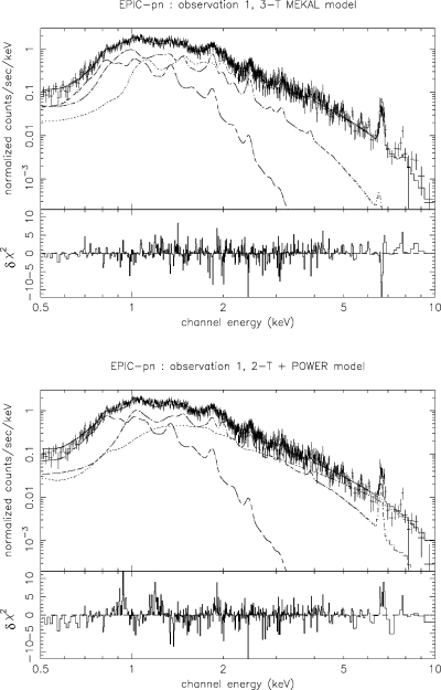
EPIC-pn spectrum of Cyg OB2 #8A of Observation 1, fitted with a wabsISM*wind*(mekal1+mekal2+mekal3) (upper panel) and a wabsISM*wind*(mekal1+mekal2+power) (bottom panel) model between 0.5 and 10.0 keV. The three components are individually displayed in both cases. The Fe K blend at about 6.7 keV is the most obvious feature in the spectrum. The bottom window of each panel shows the contributions of individual bins to the χ2 of the fit. The contributions are carried over with the sign of the deviation (in the sense data minus model).
3.4 RGS spectra
As a first step, we combined the first- and second-order spectra in order to inspect the main spectral features and to identify the spectral lines. Above about 17 Å, the spectrum is very absorbed and we concentrated our analysis on the spectral domain below this wavelength. We identified the prominent lines through a comparison with the aped (Smith & Brickhouse 2000) and spex (Kaastra, Mewe & Raassen 2004) line lists (see Table 5). In order to perform a more detailed analysis of the RGS data, we obtained fluxed (RGS1 plus RGS2) spectra for our four observations (see Fig. 3). Individual lines show intensity variations from spectrum to spectrum of a few times 10 per cent and apparent velocity variations of a few hundred km s−1, both of which are at the limit of detectability with the data available, whose exposures were typically only 20 ks. The reality of such apparent changes could be assessed with longer exposures of 60–80 ks. We insist on the fact that the strong absorption undergone by the X-ray spectrum of Cyg OB2 #8A in the RGS bandpass is a critical issue. Our attempts to derive reliable specific information such as line fluxes or velocity shifts did not provide any satisfactory result.
Identification of the prominent lines in the RGS spectrum of Cyg OB2 #8A between 6 and 17 Å.
| Ion | Wavelength (Å) |
|---|---|
| Si xiv (Lyα) | 6.180 |
| Si xiii (He-like) | 6.648 |
| Mg xii | 7.106 |
| Mg xii (Lyα) | 8.419 |
| Mg xi (He-like) | 9.169 |
| Fe xvii | 10.000 |
| Ne x (Lyα) | 12.132 |
| Ne ix (He-like) | 13.447 |
| Fe xvii | 15.014 |
| Ion | Wavelength (Å) |
|---|---|
| Si xiv (Lyα) | 6.180 |
| Si xiii (He-like) | 6.648 |
| Mg xii | 7.106 |
| Mg xii (Lyα) | 8.419 |
| Mg xi (He-like) | 9.169 |
| Fe xvii | 10.000 |
| Ne x (Lyα) | 12.132 |
| Ne ix (He-like) | 13.447 |
| Fe xvii | 15.014 |
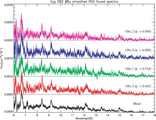
Smoothed RGS fluxed spectra of Cyg OB2 #8A obtained for our four observations between 6 and 18 Å. The orbital phase is specified in each case. The lower panel represents the mean RGS spectrum. The five spectra are, respectively, vertically shifted by 0.0005 in flux units. The prominent lines observed in the spectra are listed in Table 5.
The four RGS spectra were similar in form with no obvious changes in the long-wavelength absorption cut-off near 17 Å. Models with only interstellar absorption at the expected value of 0.94 × 1022 cm−2 are able to account for the cut-off, although we are not able to exclude a further circumstellar component for some plasma emission models. EPIC and RGS yield an effective combination with the RGS resolving lines down to Fe xvii (15.015 Å) and EPIC up to Fe xxv (18.500 Å), emphasizing the broad range of ionization conditions that exist in the X-ray emitting plasma of Cyg OB2 #8A. A similar situation was found in the X-ray spectrum of the colliding-wind system WR140 (Pollock et al. 2005). We have constructed general models involving a bremsstrahlung continuum absorbed by the expected fixed amount of interstellar material underlying line emission unconstrained by any physical plasma models from H- and He-like ions of Ne, Mg, Si, S, Ar and Ca as well as ions of Fe from Fe xvii to Fe xxv. The best-fitting continuum temperature was 1.9 ± 0.1 keV.2 In the absence of high-resolution data of good statistical weight, the same line velocity profile was used for all the lines, allowing them all to be red or blue shifted from the laboratory wavelength by the same velocity and broadened by the same velocity width. Such models are able to provide a good fit simultaneously to EPIC-MOS and RGS data (we did not consider EPIC-pn data here because of the slightly poorer spectral resolution of this latter instrument).
In addition, we used the same kind of composite models as used in Section 3.3. We subtracted the background of individual spectra and then applied the response matrix for a global fitting between 5 and 35 Å. We note that the difference in the RGS1 and RGS2 count rates reported in Table 7 stems for the dead CCD of RGS1 that falls in the 10–14 Å wavelength domain. We obtained the best fit with a two-component mekal model. The χ2 are slightly better if we use three thermal emission components but the error bars on the resulting fit parameters increase substantially. As we are dealing here with spectra containing sometimes small numbers of counts per energy bin, we used the Cash statistic (Cash 1979) to compare the results obtained with the χ2 statistic. We did not find any significant differences between the results obtained with the two approaches. We obtained typical temperatures of about 2 × 10⁶ and 8–12 × 106 K. These temperatures are close to the values obtained for the two softer thermal components of the 3-T model fitted to the EPIC data (see Section 3.3). The fact that a third emission component is not needed for data from the RGS instruments is explained by their different bandpass, i.e. 0.4 < E < 2.5 keV, whilst the ∼20 × 106 K thermal component is mostly required for higher energies. We checked the consistency of the results obtained between EPIC and RGS data through a simultaneous fit of the spectra from the four instruments, i.e. EPIC-MOS1, EPIC-pn, RGS1 and RGS2. We used the same three-temperature model as in Section 3.3 and we obtained parameter values (see Table 6) very close to those presented in Table 4 for the simultaneous fit of EPIC-MOS1 and EPIC-pn spectra, with similar or slightly larger reduced χ2.
Same as Table 4 but for RGS data fitted by a wabsISM*wind*(mekal+mekal) model between 5 and 35 Å (i.e. between 0.35 and 2.48 keV). For each observation, the results are provided for the simultaneous fit (RGS1 plus RGS2) of first-, second- and (first plus second)-order spectra. The last line for each observation gives the parameters obtained for the simultaneous fit of combined RGS (two instruments, two orders) and EPIC (MOS1 and pn) data with a wabsISM*wind*(mekal+mekal+mekal) model between 0.5 and 10.0 keV.
| log Nw | kT1 (keV) | Norm1 (10−2) | kT2 (keV) | Norm2 (10−2) | kT3 (keV) | Norm3 (10−3) | χ2ν (d.o.f.) | |
|---|---|---|---|---|---|---|---|---|
| Observation 1 | ||||||||
| RGS: Order 1 | 21.8821.9521.81 | 0.190.220.18 | 13.7724.146.12 | 1.001.060.94 | 1.521.701.35 | – | – | 1.17 (229) |
| RGS: Order 2 | 21.7621.9621.41 | 0.200.270.17 | 8.6427.021.20 | 1.381.641.25 | 1.181.410.96 | – | – | 0.93 (109) |
| RGS: Orders 1 and 2 | 21.8721.9421.78 | 0.190.200.18 | 16.2825.838.71 | 1.261.331.18 | 1.371.491.23 | – | – | 1.15 (343) |
| EPIC plus RGS | 21.6521.7021.60 | 0.240.260.22 | 2.713.821.89 | 0.780.820.76 | 0.850.930.78 | 1.761.811.71 | 8.138.597.63 | 1.39 (1243) |
| Observation 2 | ||||||||
| RGS: Order 1 | 22.0322.0921.99 | 0.230.320.19 | 9.4421.633.00 | 1.191.140.98 | 1.692.051.56 | – | – | 1.59 (217) |
| RGS: Order 2 | 21.9922.0821.90 | 0.220.280.18 | 10.4122.733.28 | 1.011.400.69 | 1.231.560.98 | – | – | 0.89 (110) |
| RGS: Orders 1 and 2 | 22.0322.0821.98 | 0.230.270.20 | 10.1218.955.18 | 1.041.100.98 | 1.641.831.46 | – | – | 1.37 (332) |
| EPIC plus RGS | 21.9021.9221.87 | 0.240.250.22 | 5.707.464.10 | 0.780.810.74 | 1.001.080.91 | 1.571.641.52 | 6.497.115.84 | 1.17 (1151) |
| Observation 3 | ||||||||
| RGS: Order 1 | 21.8421.9221.75 | 0.220.300.18 | 4.0511.091.29 | 1.051.111.00 | 1.351.531.18 | – | – | 1.13 (240) |
| RGS: Order 2 | 21.8421.9621.71 | 0.240.310.19 | 3.1710.831.17 | 1.011.070.96 | 1.251.461.15 | – | – | 1.03 (121) |
| RGS: Orders 1 and 2 | 21.8421.9121.77 | 0.220.300.18 | 3.8511.711.37 | 1.041.080.99 | 1.321.471.18 | – | – | 1.09 (366) |
| EPIC plus RGS | 21.6221.6621.57 | 0.270.330.25 | 15.0520.568.89 | 0.800.820.77 | 0.850.900.78 | 1.881.941.84 | 7.137.466.81 | 1.54 (1324) |
| Observation 4 | ||||||||
| RGS: Order 1 | 22.0021.0821.93 | 0.230.340.19 | 10.3026.412.59 | 0.921.000.78 | 1.622.161.39 | – | – | 1.17 (153) |
| RGS: Order 2 | 21.7821.9221.60 | 0.330.410.24 | 0.7317.150.34 | 0.770.870.69 | 1.581.971.36 | – | – | 0.91 (76) |
| RGS: Orders 1 and 2 | 21.9422.0221.87 | 0.290.410.19 | 3.1816.131.31 | 0.830.910.77 | 1.652.011.45 | – | – | 1.09 (234) |
| EPIC plus RGS | 21.8721.9021.83 | 0.230.250.22 | 7.8110.545.56 | 0.860.880.81 | 1.211.301.10 | 1.831.911.72 | 5.185.944.73 | 1.54 (954) |
Observed count rates of Cyg OB2 #8A for the five XMM–Newton instruments, expressed in cts s−1.
| EPIC-MOS1 | EPIC-MOS2 | EPIC-pn | RGS1 | RGS2 | |
|---|---|---|---|---|---|
| Observation 1 | 0.741 ± 0.007 | 0.737 ± 0.007 | 2.141 ± 0.013 | 0.034 ± 0.002 | 0.056 ± 0.002 |
| Observation 2 | 0.592 ± 0.006 | 0.598 ± 0.006 | 1.697 ± 0.012 | 0.027 ± 0.002 | 0.040 ± 0.002 |
| Observation 3 | 0.699 ± 0.006 | 0.692 ± 0.006 | 2.038 ± 0.011 | 0.032 ± 0.002 | 0.048 ± 0.002 |
| Observation 4 | 0.688 ± 0.008 | 0.667 ± 0.008 | 2.009 ± 0.015 | 0.035 ± 0.002 | 0.049 ± 0.002 |
4 X-RAY LUMINOSITY OF CYG OB2 #8A
4.1 Variability analysis from XMM–Newton data
The count rates obtained with the five instruments on board XMM–Newton for the four observations are quoted in Table 7. We observe significant variability of Cyg OB2 #8A on a time-scale of about 10 d, i.e. the typical separation between two pointings in our series. The largest variation is found between Observations 1 and 2, with an amplitude of about 20 per cent. We emphasize that the variations we observe for all instruments are correlated. To illustrate the variability observed between the different observations (see Fig. 4), we compared the count rates obtained in several energy bands in Observation 1 with those obtained in Observation 2 (left-hand panels), Observation 3 (middle panels) and Observation 4 (right-hand panels), respectively, for EPIC-MOS1 (upper part) and EPIC-pn (lower part). In each of these plots labelled (a)–(f), the upper section displays the count rates and the lower section shows the relative variability of the observed count rate. Although it is not shown here, we note that the same comparison was performed for the X-ray fluxes, estimated on the basis of the 3-T model with parameters given in Table 4. A plot of the relative variability of the observed X-ray flux of Cyg OB2 #8A for EPIC-pn has been presented by De Becker & Rauw (2005). We clearly see that there is a decrease in the X-ray count rate (flux) between the first and the second observation in the whole EPIC bandpass. The first and third observations appear to be very similar. In the case of the fourth observation, we see that the count rate decreases only in the hard energy band (above about 2.0 keV). We note that all the variability trends discussed here are consistent in both EPIC-MOS1 and EPIC-pn data, either if we consider count rates or observed fluxes.
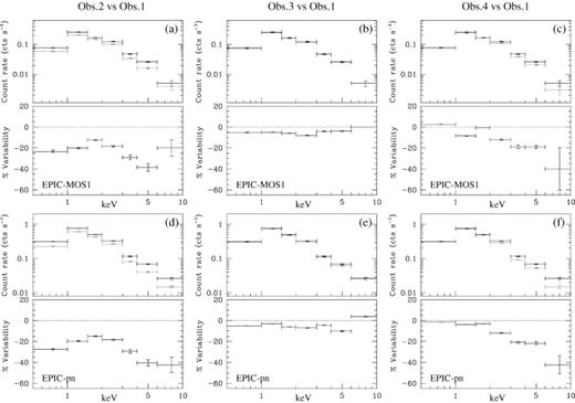
Relative variability of Cyg OB2 #8A for EPIC-MOS1 and EPIC-pn between 0.5 and 10.0 keV. For each part of the figure labelled a, b, c, d, e or f, we have represented (i) upper panels: observed count rate of the first observation (solid symbols) as compared to the nth observation (dotted symbols) with n being the number of the observation, i.e. 2, 3 or 4 and (ii) lower panels: relative variability of the observed count rate. A negative value stands for a decrease in the X-ray flux as compared to Observation 1. The vertical error bars on the count rates stand for the 1σ confidence interval, while the horizontal bars give the energy interval considered.
We finally searched for short-term variability, i.e. within a single exposure. We have binned the event lists into 100, 200, 500 and 1000 s time intervals in four energy bands, respectively, 0.5–10.0, 0.5–1.0, 1.0–2.5 and 2.5–10.0 keV. We calculated the count rates in each time bin, along with their s.d., after subtraction of a background scaled according to the respective surface areas of the source and background regions (the same as used for the spectra extraction, see Section 2.1.1). GTIs were considered to compute the count rates using effective time bin lengths. A first inspection of the light curves does not reveal any significant variability correlated between the EPIC instruments on time-scales shorter than single exposures. This lack of significant variation is confirmed by variability tests applied to every light curve (χ2 and pov-test as described by Sana et al. 2004).
4.2 Overall luminosity
On the basis of the best-fitting parameters presented in Table 4 for the three-temperature model, we have evaluated the fluxes between 0.5 and 10.0 keV for the four exposures. The observed, i.e. absorbed, fluxes are provided in the second-to-last column of Table 4. Considering a distance to Cyg OB2 #8A of 1.8 kpc (Bieging, Abbott & Churchwell 1989), we computed its unabsorbed X-ray luminosity, i.e. corrected for the ISM absorption, in the case of the simultaneous fit of EPIC-MOS1 and EPIC-pn data. The results are collected in Table 8. In this table, we also provide the LX/Lbol ratio. On the basis of the bolometric luminosities given in Table 3, we also computed the expected intrinsic X-ray luminosity using the empirical relation proposed by Sana et al. (2006). Although this latter relation relies on a rather small sample of O-type stars compared to that of Berghöfer et al. (1997), we preferred to use this one because it was established in the same energy domain as for the present analysis, i.e. between 0.5 and 10.0 keV. We therefore obtain X-ray luminosities of 3.06 × 1032 and 2.20 × 1032 erg s−1, respectively, for the primary and the secondary. The sum of these two quantities, i.e. LX of 5.26 × 1032 erg s−1, allowed us to calculate X-ray luminosity excesses ranging between about 19 and 28 (see column 4 of Table 8).
X-ray luminosity of Cyg OB2 #8A. The columns (1) and (2) yield, respectively, the flux and the luminosity between 0.5 and 10.0 keV, corrected for the ISM absorption, and derived from the simultaneous fit of EPIC-MOS1 and EPIC-pn instruments with the 3-T model. The luminosities are computed considering a distance of 1.8 kpc (Bieging et al. 1989). Column (3) gives the LX/Lbol ratio, and finally the X-ray luminosity excess is provided in column (4).
| Corrected flux (erg cm−2 s−1) | Corrected LX (erg s−1) | LX/Lbol | Excess | |
|---|---|---|---|---|
| (1) | (2) | (3) | (4) | |
| Observation 1 | 3.09 × 10⁻¹¹ | 1.20 × 1034 | 2.8 × 10⁻⁶ | 22.8 |
| Observation 2 | 2.64 × 10⁻¹¹ | 1.02 × 1034 | 2.4 × 10⁻⁶ | 19.4 |
| Observation 3 | 2.76 × 10⁻¹¹ | 1.07 × 1034 | 2.5 × 10⁻⁶ | 20.3 |
| Observation 4 | 3.73 × 10⁻¹¹ | 1.45 × 1034 | 3.4 × 10⁻⁶ | 27.6 |
5 ARCHIVE X-RAY DATA
5.1 ROSAT-PSPC data
Cyg OB2 has been observed twice with the ROSAT-PSPC instrument. A first observation was performed on 1991 April 21 (sequence number rp200109n00, ∼3.5 ks), and the second one between 1993 April 29 and 1993 May 5 (sequence number rp900314n00, ∼19 ks). The latter consisted mainly of four exposures spread over about 5 d. The analysis of Waldron et al. (1998) revealed a significant variation of the soft X-ray flux (below 2 keV) between the 1991 and the 1993 observations, with the highest emission level observed in 1993. We retrieved the screened data from the archive and we used the xselect software to analyse the data of Cyg OB2 #8A. We extracted a light curve of this observation and we split it by applying time filters to obtain four separated data sets with effective exposure times of about 3–4 ks. We selected the source events within a 1 arcmin circular region. The background was selected in an annular region around the source region of the same area, excluding its intersection with a 30 arcsec circular region centred on a point source located to the north relative to Cyg OB2 #8A (RA = 20:33:13.9 and Dec. =+41:20:21.4, Equinox 2000.0). We used the xspec software to analyse the spectra and we obtained reasonable fits with a single temperature mekal model, with a kT of about 0.5–0.7 keV. We determined the count rates for each subexposure in the 0.4–2.5 keV energy band and we collected them in Table 9, along with the time of each exposure.
Observed count rates (CR) of Cyg OB2 #8A for the ROSAT-PSPC observations expressed in cts s−1. The orbital phase is computed at mid-exposure according to the ephemeris of De Becker et al. (2004c).
| Observation | JD (−240 0000) | φ | CR (cts s−1) |
|---|---|---|---|
| rp200109n00 | 483 68.074 | 0.022 | 0.187 ± 0.008 |
| rp900314n00 #1 | 491 07.104 | 0.756 | 0.306 ± 0.014 |
| rp900314n00 #2 | 491 09.310 | 0.856 | 0.282 ± 0.010 |
| rp900314n00 #3 | 491 10.218 | 0.898 | 0.295 ± 0.007 |
| rp900314n00 #4 | 491 10.972 | 0.932 | 0.245 ± 0.008 |
5.2 ASCA-SIS data
The Cyg OB2 association was observed with ASCA (Tanaka, Inoue & Holt 1994) during the performance verification phase on 1993 April 29 (sequence number 20003000, ∼30 ks). A first analysis of these data was reported by Kitamoto & Mukai (1996). These authors already pointed out the need to use two thermal emission components, with characteristic temperatures of the order of 0.6 and 1.5 keV, respectively, in order to model reasonably the data of Cyg OB2 #8A. We retrieved the raw data and processed them using the xselect software. Even though both gas-imaging spectrometers (GIS) and solid-state imaging spectrometers (SIS) were operated during the observation, we only used SIS data because of their better spatial resolution. We extracted the source events within a 2.21 and 2.95 arcmin radius circular region, respectively, for SIS0 and SIS1. In both cases, we selected the background events from a rectangular box located a few arcmin to the east of Cyg OB2 #8A. As the source region crosses over two CCDs, we constructed two RMFs, i.e. one for each CCD, and we obtained the effective RMF through a weighted sum of the two individual response matrices.
The spectral analysis was performed with the xspec software, and the best-fitting results were obtained with the three-temperature thermal model described in Section 3.3. We note that we obtained a lower value of the reduced χ2 by replacing the third thermal component by a power law, but we estimate that this apparently better result is only due to the rather poor quality of the data in the hard part of the spectrum, unlikely to reveal the Fe K line clearly present in our XMM–Newton EPIC spectra. As the quality of the SIS0 data appeared to be significantly poorer than that of SIS1, we considered only the latter in our spectral analysis. The best-fitting parameters obtained with the 3-T thermal model between 0.5 and 10.0 keV are given in Table 10. The SIS1 spectrum and the corresponding model are presented in Fig. 5. From this model, we obtained an absorption corrected LX of 1.86 × 1034 erg s−1 between 0.5 and 10.0 keV, leading to an X-ray luminosity excess of about 35. We finally note that the observed count rate in the same energy band is 0.331 ± 0.004 cts s−1 for SIS1.
Parameters for the ASCA-SIS1 spectrum of Cyg OB2 #8A fitted with a wabsISM*wind*(mekal1+mekal2+mekal3) model between 0.5 and 10.0 keV. The parameters have the same meaning as in Table 4.
| log Nw | 21.8221.9221.73 |
| kT1 (keV) | 0.230.290.19 |
| Norm1 | 9.9130.183.98 × 10−2 |
| kT2 (keV) | 0.831.040.73 |
| Norm2 | 1.301.641.00 × 10−2 |
| kT3 (keV) | 1.662.061.46 |
| Norm3 | 7.619.831.47 × 10−3 |
| χ2ν (d.o.f.) | 1.05 (180) |
| Observed flux (erg cm−2 s−1) | 7.42 × 10⁻¹² |
| Corrected flux (erg cm−2 s−1) | 4.88 × 10⁻¹¹ |
| Corrected LX (erg s−1) | 1.86 × 1034 |
| LX/Lbol | 4.33 × 10⁻⁶ |
| LX excess | ∼35 |
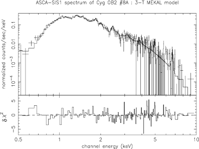
ASCA-SIS1 spectrum of Cyg OB2 #8A fitted with a wabsISM*wind*(mekal1+mekal2+mekal3) model between 0.5 and 10.0 keV. The lower part of the figure has the same meaning as for Fig. 2.
6 DISCUSSION
6.1 Orbital modulation of the X-ray flux
6.1.1 Observational material
As Cyg OB2 #8A is a binary system, one could wonder whether the existing X-ray observations reveal a modulation of the X-ray flux. This issue was first addressed by De Becker et al. (2005a) where the results from several X-ray observations (ROSAT and ASCA) were combined to obtain a phase-folded light curve, on the basis of the ephemeris published by De Becker et al. (2004c). The light curve suggested a phase-locked modulation of the X-ray flux, probably due to the combined effect of the variation of the absorption along the line of sight and of the X-ray emission itself as a function of orbital phase. Because of inconsistencies between ROSAT-HRI and ROSAT-PSPC count rates and because of a poor sampling of the orbital cycle, this preliminary light curve did not allow us to draw a firm conclusion. However, the light curve presented by De Becker et al. (2005a) suggests clearly that the ROSAT-HRI count rates show a phase modulation similar to that of the PSPC data.
Using our four XMM–Newton observations, along with the results from archive ROSAT-PSPC and ASCA-SIS1 data,3 we constructed a new light curve. To compare the count rates from the different instruments in a consistent way, we used the 3-T model with the parameters obtained for the simultaneous fit of EPIC-MOS1 and EPIC-pn data for Observation 1, and we convolved it with the respective response matrices of ROSAT-PSPC and ASCA-SIS1 to obtain faked spectra. We obtained count rates of 0.250 ± 0.004 and 0.270 ± 0.001 cts s−1, respectively, for both instruments. On the basis of these values, and of the count rates obtained in Section 5, we compared the X-ray emission level from all observations after normalization with respect to the XMM–Newton Observation 1. The normalized X-ray count rates obtained this way are plotted as a function of the orbital phase in Fig. 6. We note that this light curve does not suggest any large error on the orbital parameters derived by De Becker et al. (2004c), considering the short period and the large time interval separating some of the observations discussed here. Over the time range between 1991 and 2004, an error of 0.040 d on the period would indeed lead to an error on the orbital phase of the order of 0.4. This suggests that the error of 0.040 d given for the 21.908 d period might be a somewhat conservative value, reinforcing our confidence in the orbital parameters proposed by De Becker et al. (2004c).
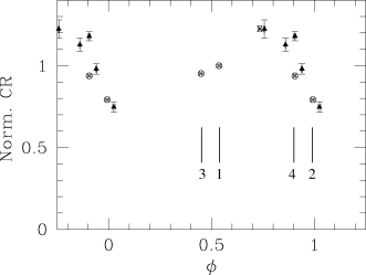
Normalized (see text) equivalent X-ray count rate of Cyg OB2 #8A from different observations as a function of the orbital phase following the ephemeris of De Becker et al. (2004c). ROSAT-PSPC: filled triangles. ASCA-SIS1: cross. XMM–Newton-EPIC: open circles. The vertical lines point to the four XMM–Newton observations labelled by their number.
The light curve of Fig. 6 presents a maximum at an orbital phase close to 0.75. We note the relative consistency of the various observations that contribute to the rather steep decrease in the X-ray emission between phases 0.75 and 1.0. We note however a discrepancy between the EPIC and PSPC points close to phase 0.9. Unfortunately, the lack of observations between phases 0.0 and 0.4 prevents us from constraining the position of the minimum, likely located shortly after phase zero. A somewhat more detailed view of the variability of the observed X-ray flux can be obtained on the basis of Fig. 7. The X-ray fluxes in the soft (0.5–2.0 keV) and hard (2.0–10.0 keV) bands are individually plotted as a function of the orbital phase in the two upper panels. In order to investigate the variability in the hard part of the X-ray spectrum, we used only XMM–Newton and ASCA data. The separation between the two stars in Cyg OB2 #8A and the position angle (PA) 4 are also provided. The decrease of the X-ray flux between apastron and periastron is particularly obvious in the hard energy band. The maximum close to phase 0.75 suggested by Fig. 6 comes mainly from the soft band, as shown by the upper panel of Fig. 7.
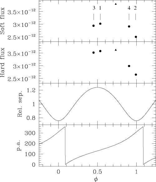
Variability of the X-ray flux of Cyg OB2 #8A as a function of the orbital phase observed with XMM–Newton (filled circles) and ASCA (filled triangle). The four XMM–Newton observations are individually labelled by their number. The four panels provide, respectively (from top to bottom), the flux between 0.5 and 2.0 keV in erg cm−2 s−1, the flux between 2.0 and 10.0 keV in erg cm−2 s−1, the relative separation between the primary and the secondary, and the PA of the system in degrees.
In addition to the decrease in the X-ray flux, the comparison between the XMM–Newton Observations 1 and 2 reveals a significant decrease in the characteristic plasma temperature of the hottest thermal component (see Table 4). As these two observations are, respectively, close to phases 0.5 (largest separation) and 0.0 (smallest separation), the decrease in the post-shock plasma temperature could be related to the decrease in the pre-shock velocity at the position of the collision zone. For this rather close binary system, the winds will indeed not yet have reached their terminal velocity before they collide. Using our estimate of the orbital (De Becker et al. 2004c) and wind (Table 3) parameters and adopting a β= 1 wind velocity law, we calculate the distance between the stagnation point (i.e. the location of the wind–wind interaction on the binary axis) and the centre of each star. Following an estimate of the inclination angle of the system,5 i.e. about 32°± 5°, we infer absolute distances of about 95 and 81 R⊙, respectively, for the primary and the secondary at apastron (respectively 58 and 50 R⊙ at periastron). Using the corresponding pre-shock velocities, we expect the post-shock temperature to vary (on-axis) between about 35 × 106 and 25 × 106 K from phases 0.5 to 0.06 (see Table 11). According to the values quoted in Table 4, the observed temperature for the hottest thermal component is about 21 × 106 and 18 × 106 K, respectively, for Observations 1 and 2. The fact that the predicted and observed temperatures are different (about a factor of 1.4–1.7) may suggest that the effective pre-shock velocity is lower than predicted by about a factor of 1.2–1.3. However, as the EPIC bandpass does not extend further than 10 keV, we should bear in mind that our spectral fits may underestimate the characteristic temperature of the post-shock plasma. Moreover, some fraction of the emission is expected to come from off-axis where the shocks are oblique, leading the averaged observed emission to have a lower characteristic temperature than anticipated at the stagnation point. Finally, some radiative inhibition (Stevens & Pollock 1994) may be at work close to the line of centres of the binary system, therefore reducing the speed of the wind flows before they collide. As a result, considering the numbers given above, we consider that the agreement between the temperatures estimated from the fit of our X-ray spectra and that derived from the geometry and hydrodynamic of the colliding winds in Cyg OB2 #8A is very satisfactory.
Stand-off distances (d), pre-shock velocities (Vpre-shock), post-shock temperatures (Tpost-shock) and cooling parameters (χ) calculated at the three orbital phases selected for the hydrodynamic simulations, respectively, for the primary (1) and the secondary (2) of the system. The velocities were calculated on the basis of the terminal velocities and radii provided in Table 3, using a β= 1.0 velocity law. We note that, as the estimate of the pre-shock velocities depends on the radius of the stars, the uncertainty on this latter quantity might be responsible for uncertainties on the calculated pre-shock velocities, and therefore on the post-shock temperatures as well.
| Orbital phase (φ) | 0.5 | 0.75 | 0.0 |
|---|---|---|---|
| d1 (R⊙) | 95 | 81 | 58 |
| d2 (R⊙) | 81 | 69 | 50 |
| Vpre-shock,1 (km s−1) | 1478 | 1408 | 1222 |
| Vpre-shock,2 (km s−1) | 1722 | 1655 | 1485 |
| Tpost-shock,1 (MK) | 30 | 27 | 20 |
| Tpost-shock,2 (MK) | 40 | 37 | 30 |
| χ1 | 0.66 | 0.46 | 0.19 |
| χ2 | 1.65 | 1.20 | 0.57 |
Some explanation for the variability described in Section 4.1 (see Fig. 4) and in Figs 6 and 7 can be given on the basis of the different orbital phases of our XMM–Newton observations. In the case of a binary system like Cyg OB2 #8A, we can expect some variability in the X-ray domain mainly for two reasons described as follows.7
The variation of the line-of-sight absorption along the orbital cycle, likely to affect mostly the softer part of the spectrum (i.e. below about 2.0 keV).
The variation of the separation between the two stars, as the orbit is eccentric, likely to affect the physical conditions in the colliding wind zone. If some variability is observed in the harder part of the spectrum, it should most probably come from this process.
Considering the strong differences between Observations 1 and 2 in the whole EPIC bandpass (parts a and d of Fig. 4), both factors might play a significant role. Considering only XMM–Newton results, this decrease is more spectacular in the hard part of the spectrum (Figs 4 and 7). This should be due to the variation of the separation between the two stars. The fact that Observation 2 occurs when the primary is ‘in front’ of the secondary (PA close to 0°), i.e. at an orbital phase where the absorption should be larger, may explain the decrease in the soft part of the spectrum. The parameters quoted in Table 4 point indeed at a higher local absorption column in the case of Observation 2 as compared to the first one. The same trend is also suggested by the fits of RGS spectra (see Table 6). The lack of significant variability between Observations 1 and 3 (parts b and e of Fig. 4) is compatible with the fact that they fall nearly at the same phase close to apastron. Finally, the decrease in the X-ray emission observed above 2.0 keV in Observation 4 (parts c and f of Figs 4 and 7) might be explained by the decrease in the separation, lowering the X-ray emission from the collision zone. The somewhat higher local absorption in the case of Observation 4 suggested by the wind absorption parameter given in Table 4 may be an artefact of the fit, where the apparent higher absorption is compensated for by the larger normalization parameter of the same observation.
6.1.2 Hydrodynamic simulations
Considering the light curves presented above (see Figs 6 and 7), it is obvious that the X-ray emission from Cyg OB2 #8A presents orbital modulations which are worth to be further investigated. For a better understanding of the physical processes responsible for this orbital modulation, we compared our XMM–Newton observations with the predictions of detailed hydrodynamic simulations using the same approach as Sana et al. (2004). In this method, the VH-1 numerical code based on the piece-wise parabolic method (Colella & Woodward 1984), is used to solve the partial differential equations of hydrodynamics followed by a remap on to a fixed grid after each time-step. A radiative energy loss term is included in the hydrodynamic equations in order to treat the cooling self-consistently. For details see Stevens et al. (1992), Pittard & Stevens (1997) and Sana et al. (2004).
Briefly, two spherically symmetric ionized winds of constant velocity are assumed, resulting in an axisymmetric geometry around the lines of centres where the hydrodynamic problem is reduced to a two-dimensional flow. The orbital motion is neglected. As the acceleration of the wind is not taken into account, the pre-shock velocity is estimated on the basis of a classical velocity law (β= 1.0), for a terminal velocity estimated to be 2.6 times the escape velocity (Vink et al. 2000). We adopted a square grid size of 300 × 300 cells, corresponding to physical distances of 1.5 × 1013×1.5 × 1013 cm and we let the flow evolve a time long enough so that the system relaxes from the initial conditions. At each step, grids of density, pressure, radial and axial velocities are obtained, and therefore grids of temperature can be calculated. The X-ray emission from the system is evaluated by summing up the emissivity of each cell of the grid at each time-step. The column of absorbing material was computed following a three-dimensional geometry taking into account the inclination of the system and the orientation of the line of sight with respect to the system (see Sana et al. 2004, for details).
We chose three different system configurations to evaluate the evolution of the X-ray flux between 0.5 and 10.0 keV along the orbital cycle: (i) apastron (φ= 0.5), (ii) intermediate (φ= 0.75) and (iii) periastron (φ= 0.0). The pre-shock velocities, the post-shock temperatures and the cooling parameter (χ) estimated in each case are given in Table 11 for both stars of the system. In the three cases, the collision zone relaxes from initial conditions after about 2500 steps, i.e. about 4 × 10⁵ s, and turns out to be highly unstable. This instability comes most probably from the cooling as the shock of the primary wind, and that of the secondary at periastron, are radiative (Stevens et al. 1992), as suggested by the values quoted for the cooling parameter (χ) in Table 11. We mention also that it may also partly result from shear instabilities as the winds in Cyg OB2 #8A have different velocities.
The mean and s.d. of the X-ray luminosity are computed over a large number of time-steps after relaxation from the initial conditions. The averaged predicted X-ray luminosities, absorbed by both the wind and the interstellar material (using NH= 0.94 × 1022 cm−2, see Section 3.2), are given in the second column of Table 12. The comparison of the predicted and observed X-ray luminosities reveals that the theoretical modelling leads to X-ray luminosities in reasonable agreement (within about a factor of 2) with the observed luminosities. The simulations predict also a minimum of the X-ray luminosity at periastron that is consistent with what we observe (see Fig. 6). The rather high emission level observed close to phase 0.75 is also predicted. We mention that the observed large amplitude of the variation between phases 0.75 and 0.0 is also predicted, even though this amplitude is larger for the predicted values. In addition, the relative emission levels obtained at the three orbital phases selected for our simulations are in reasonable agreement with the fluxes plotted in Fig. 7 in the hard energy band, i.e. the spectral domain where the colliding winds are mainly expected to produce X-rays. In particular, the rather similar emission levels obtained at phases 0.5 and 0.75 is in agreement with the observed hard X-ray fluxes. In addition, we mention that the results of the simulations are in agreement with the large X-ray overluminosity revealed by the observations. The rather good agreement of the general behaviour between the predicted and observed variabilities confirms that the observed orbital modulations of the X-ray flux are produced by the line-of-sight absorption and by the variation of the separation between the two stars, as these two effects are dominant in our simulations. This result provides strong support to the scenario where the modulations of the X-ray flux come from the colliding winds.
Predicted absorbed fluxes of Cyg OB2 #8A at three characteristic phases of the orbital cycle. The observed X-ray fluxes obtained close to the three phases are also quoted for comparison. For this latter quantity, the satellite is specified in each case. The observed fluxes are taken from Tables 4 and 10.
| Phase (φ) | fX,sim (erg cm−2 s−1) | fX,obs (erg cm−2 s−1) |
|---|---|---|
| 0.5 | (1.15 ± 0.30) × 10−11 | 0.66 × 10⁻¹¹ (XMM #1) |
| 0.75 | (0.90 ± 0.25) × 10−11 | 0.74 × 10⁻¹¹ (ASCA) |
| 0.0 | (0.42 ± 0.12) × 10−11 | 0.52 × 10⁻¹¹ (XMM #2) |
| Phase (φ) | fX,sim (erg cm−2 s−1) | fX,obs (erg cm−2 s−1) |
|---|---|---|
| 0.5 | (1.15 ± 0.30) × 10−11 | 0.66 × 10⁻¹¹ (XMM #1) |
| 0.75 | (0.90 ± 0.25) × 10−11 | 0.74 × 10⁻¹¹ (ASCA) |
| 0.0 | (0.42 ± 0.12) × 10−11 | 0.52 × 10⁻¹¹ (XMM #2) |
6.2 Non-thermal emission
Cyg OB2 #8A is known as a bright non-thermal radio emitter (Bieging et al. 1989). The fact that it is a confirmed binary system suggests that the non-thermal emission is produced in the wind interaction zone. This has recently been confirmed by Blomme (2005) who presented a phase-folded radio light curve built on the basis of new data showing a strong phase-locked variability of the radio flux density. This is in agreement with the results of the study of Van Loo, Runacres & Blomme (2006) who showed that the production of the observed non-thermal emission from isolated stars is unlikely. In this scenario, electrons are accelerated through the first-order Fermi mechanism up to relativistic velocities (Eichler & Usov 1993). This population of relativistic electrons is expected to interact with the local magnetic field, likely originating from the two stars, to produce synchrotron radiation in the radio domain (see e.g. Dougherty et al. 2003). New developments in the modelling of non-thermal radio emission from massive binaries are described by Pittard et al. (2006). These recent models take into account several physical effects like free–free absorption, the Razin effect and IC cooling.
The latter process is particularly interesting in the sense that the cooling of relativistic electrons by UV photospheric photons through IC scattering is likely to produce a non-thermal high-energy emission component. However, we did not find any evidence for a power-law emission component attributable to a non-thermal emission in our XMM–Newton-EPIC spectra of Cyg OB2 #8A. This was not unexpected as any putative non-thermal emission component would probably be overwhelmed by the strong thermal emission arising from the wind–wind interaction zone. The unlikelihood of the detection of a power-law emission below 10.0 keV in the case of non-thermal radio emitting massive binaries was indeed pointed out by De Becker et al. (2005b). However, such a non-thermal emission could possibly be detected in very hard X-rays and soft γ-rays, where the spectra are not expected to be contaminated by thermal emission. For instance, De Becker et al. (2005a) estimated that the possible contribution of Cyg OB2 #8A to the γ-ray emission from the yet unidentified EGRET source 3EG J2033+4118 could amount up to about 10 per cent. However, these estimations need to be refined using more sophisticated models (see e.g. Pittard & Dougherty 2006). In addition, the observation of the Cyg OB2 region with the IBIS(ISGRI) imager onboard the INTEGRAL observatory did not allow to detect any high-energy emission putatively associated to the massive stars in Cyg OB2 (De Becker 2005).
7 SUMMARY AND CONCLUSIONS
In this paper, we presented the results of four XMM–Newton observations of the massive binary Cyg OB2 #8A separated by about ten days from each other. The best fits of the X-ray spectra were obtained using a three-temperature thermal model, with characteristic plasma temperatures for the three components of about 3 × 10⁶, 9 × 10⁶ and 20 × 106 K. The hottest component is most probably attributed to the thermal X-ray emission from the collision zone between the winds of the two stars. The nature of the X-ray emission appears to be purely thermal, and we failed to fit power-law models to the hard part of the spectrum. This is in agreement with the idea proposed by De Becker et al. (2005b) that non-thermal radio emitters are not likely to display a non-thermal emission component in their X-ray spectrum below 10.0 keV. The X-ray luminosity is very high (about 1034 erg s−1, leading to an X-ray luminosity excess of 19–28 during our observations). This rather high X-ray emission level is in disagreement with the statement by Waldron et al. (2004) that the X-ray emission in Cyg OB2 #8A is probably not different from that expected from isolated O-stars.
The analysis of high spectral resolution RGS data reveals an absorbed spectrum with prominent lines mainly from Si xiv, Si xiii, Mg xii, Mg xi, Ne x, Ne ix and Fe xvii. The comparison of the spectra obtained at different orbital phases suggests a possible variability of some line profiles. A better phase coverage of the orbital cycle with much longer exposure times is needed to address this issue in detail.
We folded the count rates from our XMM–Newton observations, along with those from archive ROSAT-PSPC and ASCA-SIS observations, with the ephemeris given by De Becker et al. (2004c). We observe a variability of the count rate and of the X-ray flux of about 20 per cent between apastron and periastron. The light curve as a function of the orbital phase points to a maximum at about phase 0.75, and suggests a minimum shortly after the periastron passage. The shape of the light curve might be explained by the combined effect of absorption and varying separation along the orbital cycle, this latter factor being responsible for the lower pre-shock velocity reached by the winds at periastron with respect to apastron. Using hydrodynamic simulations, we also find a lower emission level close to phase 0.0. The amplitude of the observed variation is less than predicted. This contrast may be reduced by including shock modification (Pittard & Dougherty 2006), by reducing the value of β for the wind velocity law, or even by slightly changing the inclination angle. As a main conclusion, we state that the strong phase-locked variability — along with the spectral shape — of the X-ray emission of Cyg OB2 #8A revealed by our investigation points undoubtedly to X-ray emission dominated by colliding winds.
In the future, Cyg OB2 #8A appears to be an ideal target for the Wide-band X-ray Imager (WXI) and the Soft Gamma-ray Detector (SGD) onboard the Next-generation X-ray Telescope satellite NeXT (Takahashi et al. 2004), whose sensitivity is expected to be significantly better than that of INTEGRAL. On the other hand, the results from the radio monitoring of Cyg OB2 #8A (Blomme 2005) might be used in parallel with state-of-the-art models to evaluate the non-thermal emission level in the high-energy domain.
The rmfgen task may not work properly when confronted to somewhat complicated source regions made of circles and boxes such as shown in Fig. 1. See the XMM helpdesk message ID SASv6.0/16904 at http://xmm.vilspa.esa.es/xmmhelp for details.
For a pre-shock velocity of the order of 1500 km s−1 (see Table 11) and solar abundances, one could expect the post-shock temperature to be of the order of 2.6 keV, but the lower value derived from the fit may be due to the fact that a large fraction of the post-shock plasma is located off-axis. In this case, the component of the pre-shock wind velocity that contributes to the heating of the plasma is only a fraction of the total pre-shock wind velocity, i.e. the component of the wind velocity that is perpendicular to the shock surface.
As we suspect some problems in the calibrations of the HRI instruments relative the PSPC, we do not consider ROSAT-HRI count rates in our discussion.
This PA is 0° when the primary is in front of the secondary, and is 180° in the reverse situation. The longitude of the periastron (ω), that is required to compute the PA, is equal to 220°± 12°. This result was not mentioned in De Becker et al. (2004c).
We estimated the inclination angle by comparing the minimum masses given by De Becker et al. (2004c) and the typical masses given by Martins et al. (2005) for stars of the spectral type and luminosity classes of the components of Cyg OB2 #8A.
These temperatures correspond to the mean of the post-shock temperatures obtained, respectively, for the primary and the secondary. These temperatures are maximum values as they are estimated along the line of centres.
We also mention that some variability may be expected if the wind collision crashes on to the surface of the secondary (see e.g. Pittard 1998 and Sana et al. 2005), but we do not expect this scenario to occur in the case of Cyg OB2 #8A as the wind collision zone is not located close enough to the surface of the secondary.
Based on observations with XMM–Newton, an ESA Science Mission with instruments and contributions directly funded by ESA Member states and the USA (NASA).
ACKNOWLEDGMENTS
Our thanks go to Alain Detal (Liège) for his help in installing the sas. The Liège team acknowledges support from the Fonds National de la Recherche Scientifique (Belgium) and through the PRODEX XMM and INTEGRAL Projects. This research is also supported in part by contract P5/36 ‘Pôle d'Attraction Interuniversitaire’ (Belspo). This research has made use of the SIMBAD data base, operated at CDS, Strasbourg, France and NASA's ADS Abstract Service.
