Beware λ-truncation! Sample truncation and bias in luminosity calibration using trigonometric parallaxes

Abstract

1 Introduction

At present the aim of luminosity calibration for some given class of stars is essentially to estimate the ‘typical’ absolute magnitude for the class (and, sometimes, the dispersion). Conventionally this is done assuming a Gaussian (realistically, a truncated Gaussian) distribution parametrized by a mean and a standard deviation. In some situations one may have a functional relation between luminosity and some observed quantity such as period for Cepheid variables which one wishes to calibrate. While this may introduce additional complications and more parameters, the fundamental problem remains the same.

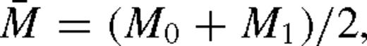
The desired mean is often taken to be that appropriate to a sample restricted to a certain volume of space, frequently referred to as the ‘mean per unit volume’ and denoted by M₀. Alternatively one may estimate the mean for a sample that is limited according to the value of some observed quantity such as apparent magnitude m, which mean is sometimes designated M₁. The former is considered more fundamental because the specification does not explicitly refer to a particular value of some observed quantity. Of course, as a practical matter one must in some way use such quantities to identify those stars that may lie inside the specified volume, e.g. by choosing those that have measured parallaxes π ′ larger than a certain lower limit π ′_l (a rather crude method). Such a sample has sometimes been referred to as ‘volume-limited’ but is more correctly termed ‘parallax-limited’ because of the parallax random errors.

The custom of calling the difference (M₁−M₀) the Malmquist ‘bias’ is in our view mistaken. If the second sample above is explicitly truncated according to m alone (ignoring photometric errors) then M₁ is by definition the actual mean for that sample, and to the extent that the parallax-limited sample approaches a true volume-limited sample any difference between the two means is not really a bias in the traditional sense of some systematic error in the measurements or in the methodology. The means are for two differently defined samples. We can speak of a bias only if the estimator for M₁ is naively interpreted as an estimator for M₀.¹

Our objection to the use of the term ‘bias’ in the context of the Malmquist effect is no mere quibble. One should always keep in mind that a systematic difference may exist between the actual sample mean and the desired mean, for instance M₀, particularly when sample selection is based on some observed quantity in addition to, or other than, the primary one, in the present instance π ′. Such a difference, if it exists, is not properly termed a bias; perhaps a more appropriate (and neutral) term is offset. The Malmquist ‘bias’ affords a ready example. In this paper the term bias will be applied solely to systematic differences between estimated means and their corresponding actual values. (The same reasoning of course applies to other estimators such as most probable values.) Moreover, the term ‘correction’ implies that one estimate is incorrect; the term shift is more appropriate in the case of an offset.

Truncation of a parallax sample at π ′_l as described above introduces a well-known bias (Trumpler & Weaver 1953) into the mean of the absolute magnitudes M′ calculated directly from those parallaxes, in the so-called direct method of luminosity calibration. The expected negative slope of the distribution of true parallaxes together with the truncation causes an excess of positive parallax errors for the truncated sample so that the mean is expected to be larger than the true mean (which approximates M₀ to within the sampling error). Any systematic difference between the two is thus an example of a true bias, not an offset.

To counter this bias, Lutz & Kelker (1973) calculated magnitude corrections as a function of the relative parallax error σ_π/ π ′, which we denote λ, to be applied to individual stars in a sample on the assumption of uniform space density; here σ_π is the estimated standard error of the parallax. A fixed upper limit λ_u = 0.175 had to be imposed because the correction could not be calculated for larger values. This λ-truncation, as we call it, introduces a bias with the direct method (Arenou & Luri 1999; Pont 1999) which is essentially the same (Smith 2003, hereafter S03) as the Trumpler-Weaver bias, being identical when the σ_πs of all stars are the same. The Lutz-Kelker corrections should eliminate it provided that the assumption of uniform density is correct and that the sample is strictly truncated by λ only. Unfortunately these conditions are not always satisfied, necessitating either modification of the corrections or some other approach. One can estimate the power law (assuming that one applies) for the spatial distribution from the proper motion distribution (Hanson 1979) and modify the corrections, or one can estimate them differentially (Sandage & Saha 2002).

To avoid Trumpler-Weaver bias altogether, Arenou & Luri (1999) and Pont (1999) recommended using the well-known method of reduced parallaxes (RP method) with a magnitude-limited sample instead of the direct method with λ-truncation and Lutz-Kelker corrections. Then on average the positive and negative parallax errors cancel out. In addition, non-positive parallaxes can be included in the solution, whereas they cannot with the direct method. Of course in this case RP estimates M₁ rather than M₀, so if the latter is desired a Malmquist shift must be applied. Also, as was shown in S03 the method is based on a linear approximation and therefore has a modelling bias.

The truncation bias can also be avoided by using the grid method from S03 with a magnitude-limited sample, either in the original form to get M₀ or in the modified form from S03 to get M₁. (The former has a Malmquist shift essentially built-in.) Both Jung's (1971) method referred to in S03 and the grid method were intended for such samples, but this fact was not made explicit in that paper. Like the RP method, it can handle non-positive parallaxes. The RP method, Jung's method and the grid method are all maximum likelihood (ML) methods.

Although λ-truncation is somewhat problematic, in the literature we find a number of papers on calibration that employ it either explicitly or implicitly, in the form of an upper limit on the absolute magnitude error ε_{M, u}. If the photometric error in apparent magnitude is negligible, the magnitude error can be shown to be approximately ε_M = 2.17λ so that the criterion ε_{M, u} = 0.25 is roughly the same as λ_u = 0.115. (If the photometric error is included in the cut-off, the restriction on λ is rendered even more strict.) Recently a common choice for λ_u itself has been 0.1 rather than 0.175 or 0.2, presumably in the belief that smaller λ_u will yield more accurate results. Although generally this is true, it is not true in all cases, as we show below.

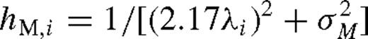
Another way of restricting a sample with RP is truncation according to weight, as in Feast & Catchpole (1997, hereafter FC). Denoting weight by h, we will term this h-truncation. The quantities λ and h are not related in a straightforward way, so any bias from h-truncation (if it exists) may not behave in the same manner as that from λ-truncation.

In this paper we assume that all samples are m-truncated, and examine what happens with additional truncation by λ with the grid and RP methods (in the next section) or by h with the RP methods (in Section 4). For comparison we consider the bias introduced by λ-truncation with the direct method and two variants of that method (Section 3). In the last section we discuss the ramifications of these results.

2 Truncation By Both λ and m with Indirect Methods

2.1 The true mean

Consider the idealized case in which a sample is chosen from a population of stars of a given type randomly distributed through three-dimensional space with uniform density. To facilitate comparison with the results in our earlier papers (Smith 1987b, Paper IV; Smith 1988, Paper V), we choose parallax standard error 30 mas and a luminosity function which is Gaussian-truncated at ±3σ_M with mean M₀ = 10 and specified dispersion σ_M. The sample is selected with 0 < λ≤λ_u and m≤m_l; we vary m_l while λ_u is fixed at the Lutz-Kelker value 0.175.

Fig. 1 shows how the true sample mean varies with m_l for two values of σ_M, namely 0.3 and 0.8. For small m_l the mean has the Malmquist value M₁ =M₀− 1.38σ²_M, changing to M₀ at large m_l.

Figure 1

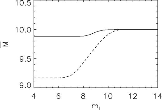
Sample mean absolute magnitude as a function of limiting apparent magnitude m_l for λ-truncated samples having M₀ = 10 and absolute magnitude dispersion σ_M = 0.3 (solid curve) or 0.8 (dashed curve) when M₀ = 10; parallax error σ_π = 30 mas for both.

Open in new tabDownload slide

This transition from ‘magnitude-limited’ samples dominated by m-truncation at small m_l to ‘parallax-limited’ samples controlled by λ-truncation at large m_l was already described by Lutz (1983). We speculated in Paper IV that the transition from one to the other should occur around a value

(1)

where π _LK≡σ_π/0.175, and that the width of the transition region is 4 mag. The figure shows that both speculations were incorrect, albeit to differing degrees. If we choose for the empirical transition value that m_l for which , we find that for σ_M = 0.3 it is m_t,e = 8.89, while for σ_M = 0.8 we have m_t,e = 8.60; the theoretical value from Paper IV, which is the same for both, is 8.83. The value of m_t,e is therefore weakly dependent on σ_M. On the other hand, the range of the transition is strongly dependent on σ_M: for σ_M = 0.3 it is about 2 mag, while for σ_M = 0.8 it is roughly 5 mag. We would naively expect the range to be about 6σ_M based on the form of the luminosity function, which is approximately consistent with the data (actual ranges may be slightly larger).

As we demonstrated in Paper IV, the Lutz-Kelker corrections are only valid (if at all) in the regime where λ-truncation dominates. For small m_l, where m-truncation dominates, no correction is necessary and the Lutz-Kelker corrections are not appropriate. In the transition region where the true mean lies between M₁ and M₀, the directly calculated mean will differ from it by less than the Lutz-Kelker amount — the actual bias — and in addition the true mean will differ from M₀ and M₁ by non-zero offsets, one negative and the other positive.

2.2 Estimation using the grid method

As a test we applied the grid method discussed in S03 to 10 synthetic samples having the parameters M₀ = 10, m_l = 12, σ_π = 30 mas, N = 1000 and various values of σ_M, and truncated using λ_u = 0.175. As Fig. 1 shows, these samples are parallax-limited. Accordingly the version of the grid method without the built-in Malmquist shift was used. The results are presented in Table 1. (The last row corresponds to the case considered at length in S03, which in that paper was not λ-truncated.)

Table 1

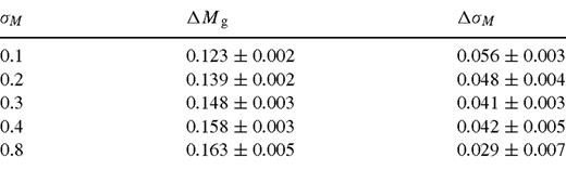
Bias in M₀ and σ_M using grid method with λ-truncation, synthetic data with λ_u = 0.175.

Open in new tabDownload slide

The bias ΔM_g increases with increasing σ_M but only gradually. Because the bias is caused by the parallax errors, we expect it to be present even if σ_M = 0. The bias Δσ_M, which is smaller, actually decreases (but very slowly) as the true σ_M is increased. Perhaps the explanation for this latter behaviour lies in the fact that for large σ_M the spread in parallax relative to that parallax for which M =M₀ (i.e. the spread due to σ_M) frequently exceeds the spread of the parallax errors, thus lessening the effect of the latter. In any event, quite clearly the original grid method is inappropriate for λ-truncated samples and must be modified if one wishes to take the truncation into account. In the last section we shall return to this consideration.

2.3 Estimation of the mean using RP methods

In S03 we considered three ML calibration methods based (as we showed) on a linear approximation for the case when the spread in parallax caused by the errors is assumed to be greater than that arising from the spread in absolute magnitude. Two of these had been used in the past, the other being (so far as we knew) new. One of the two is the asymptotic unbiased estimation (AUE) method of Turon & Crézé (1977) and the other is the method described in FC, which we have referred to (in S03) as the FC method. The third method is the p-method derived in S03. All three are essentially least-squares methods fitting the measured parallaxes to photometric parallaxes, both scaled according to m, with the mean absolute magnitude as the parameter; they differ only in the form of the weights h used. (This scaling of the parallax is the reason for the appellation ‘reduced parallaxes’ applied to such methods.) The basic RP formula is

(2)

where p_i≡α_i π ′_i and the scale factor α_i≡ dex [0.2m_i+ 1]. The AUE method uses a weight of the form

(3)

while the weight with the FC method is

(4)

and that for the p-method is

(5)

with the photometric parallax . In S03, 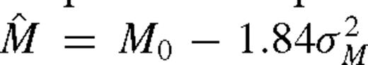was formally associated with the most probable parallax for a purely magnitude-limited sample from a uniform three-dimensional spatial distribution. In practice it is the parameter to be found in the solution, although it clearly differs from M₁ by an offset −0.46σ²_M for magnitude-limited samples and has a modelling bias noted in S03 of 0.69σ²_M, for a net of 0.23σ²_M. For convenience we will continue referring to the combination of the two as ‘modelling bias’. Even though the weights in equations (3)–(5) look rather similar (as remarked in S03), it turns out that the differences can be important.

We estimate for samples having the same parameters as in the preceding subsection except for σ_M = 0.8, which as in S03 we consider well outside the range of the linear approximation underlying the method. To simplify matters we take the true value of σ_M as given rather than solving for it in addition to . The bias values obtained with the formulations above are given in Table 2. They do not include any bias correction, e.g. for modelling bias. Comparing the bias values from the variants, we see that the FC method and the p-method give similar values for the smallest value of σ_M, whereas the value from the AUE method is somewhat different. For larger values of σ_M the estimates from the AUE and FC methods both deviate markedly from those from the p-method, trending downward instead of upward. For σ_M≥ 0.5 the biases with the AUE and FC methods are both negative.

Table 2

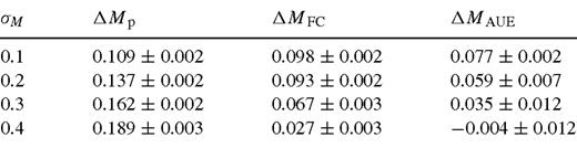
Bias of RP methods with λ-truncation, synthetic data with λ_u = 0.175.

Open in new tabDownload slide

The biases ΔM_g with the grid method in Table 1 differ noticeably from the corresponding values from the p-method in Table 2, whereas from S03 one might have expected them to be comparable (to within the modelling bias 0.23σ²_M). The differences are partly because with the latter the value of σ_M was fixed at the true value whereas with the former it was solved for. If we use the grid method with the correct σ_M fixed we get much the same bias as with the p-method at small σ_M (again allowing for the modelling bias).

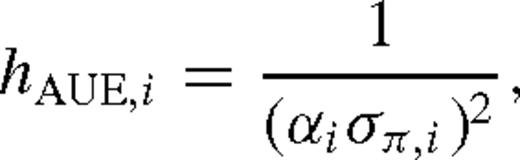
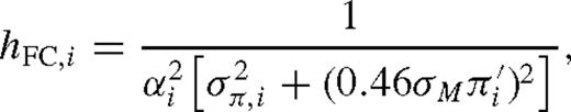
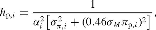
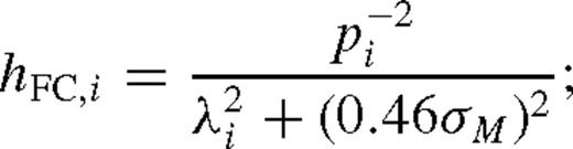
Since the sets of synthetic parallaxes used were the same for all three variants of the RP method with each selection of parameter values, and the basic formula used was the same for all three, the differences in the results must have arisen solely from the differences in the weights. These differences arise because the second terms in brackets in equations (4) and (5) are not completely negligible compared with σ²_π for all stars; otherwise the weights h_FC and h_p would be identical to h_AUE. Those terms are relatively large when σ_M differs substantially from zero and if λ is small. A star that roughly satisfies λ < 0.46σ_M will have differing weights, with h_AUE being largest. The nearest stars of a given sample, which are the most likely ones to satisfy this condition, are also the ones with the smallest m_i and therefore the largest h_AUE,i∝ dex [−0.4m_i]. The emphasis given those relatively few stars, together with the spread arising from σ_M, probably accounts for the lower efficiency of the AUE method for non-zero σ_M compared with other methods, as indicated by the uncertainties in Table 2 and as remarked previously (Smith 2001).

In our opinion, the best way to visualize these differences is by plotting the scaled parallaxes p_i against the respective weights h_i. In Figs 2(a)–(c) we do just that for a synthetic sample of 4000 stars having σ_M = 0.4 using the three variants. The distributions in the h–p diagrams for the FC and AUE methods look somewhat similar; however, the factor of 2 difference in horizontal scales for the two means that the scatter in h is smaller for the former. The distribution for the p-method has a clearly defined upper bound on h, unlike the other two. In all three cases there is a sharply defined lower envelope created by the λ-truncation. The shapes of the envelopes are significantly different, however, as shown in the Appendix and as may be seen in the figures.

Figure 2

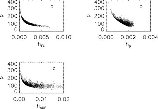
Graph of scaled parallax p (see text) versus weight h for a synthetic sample of 4000 stars having M₀ = 10, σ_M = 0.4, σ_π = 30 mas and λ_u = 0.175 with the three variants of the RP method: (a) FC method; (b) p-method; (c) AUE method. Note the different horizontal scales.

Open in new tabDownload slide

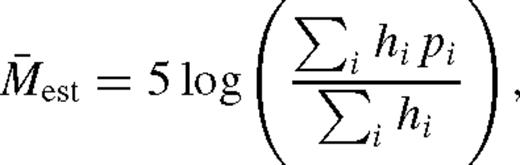
The distributions in Fig. 2 suggest a way to understand at least in part the biases in Table 2. The λ-truncation, which largely cuts off smaller values of p, tends to bias the result towards larger M. However, the FC and AUE methods seem to give high weight especially to p-values below 100 (the nominal value of p, roughly equal to ), tending to compensate (or overcompensate) for the bias from the λ-truncation and thereby sometimes to underestimate M. Indeed, the smaller values of p tend to be those for intrinsically brighter stars, especially with large σ_M. The p-method, which assigns weights with a well-defined upper bound and is therefore mainly affected by λ-truncation, consistently overestimates M.

2.4 Dependence of bias on λ_u

Thus far we have for convenience used the Lutz-Kelker value of λ_u. As we commented in the Introduction, however, a more fashionable value to use is 0.1, which raises the question of how the bias depends on λ_u. Figs 3(a)-(c) answer that question for the RP methods. For all but the smallest value of σ_M, the bias is negative for values of λ_u smaller than 0.175 when the FC and AUE variants are used. Since, as was noted above, the bias becomes negative for larger σ_M with λ_u = 0.175, this should come as no surprise. However, the absolute value of the bias generally increases as λ_u decreases, which is surprising. With the p-method, on the other hand, the bias is uniformly positive and decreases as λ_u decreases. Indeed, in that case the values for the different σ_M asymptotically approach the respective modelling bias values 0.23σ²_M.

Figure 3

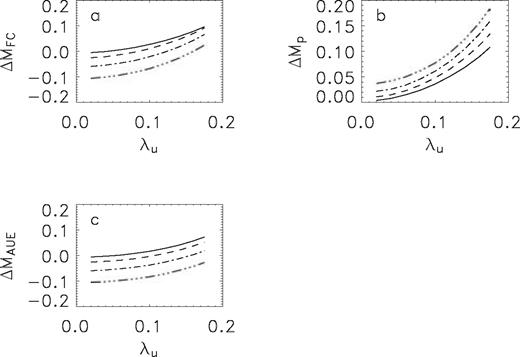
Bias ΔM for the RP methods as a function of λ_u: (a) FC method; (b) p-method; (c) AUE method. The curves are for different values of σ_M: solid curves for σ_M = 0.1; dashed curves for 0.2; dot-dashed curves for 0.3; triple-dot-dashed curves for 0.4. Note that vertical scale in (b) differs from those in (a) and (c).

Open in new tabDownload slide

The different behaviours of the biases with varying λ_u are linked to the differences between their respective λ-truncation envelopes, which are shown in Figs 4(a)-(c) for three different values of λ_u. As λ_u is reduced, the envelopes for the FC and AUE methods increasingly exclude the larger values of p, leaving only the smaller values of highest weight and causing a growing underestimation. At the same time, the envelope for the p-method becomes more nearly vertical and does not emphasize the larger p-values as much as with larger λ_u. Thus the overestimation declines.

Figure 4

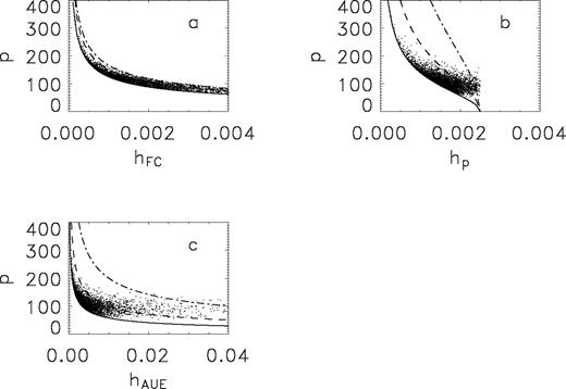
As Fig. 2 but with λ-truncation envelopes superimposed for three values of λ_u: solid curve λ_u = 0.175; dashed curve λ_u = 0.1; and dot-dashed curve λ_u = 0.05.

Open in new tabDownload slide

The preceding does not really explain why the bias is negative with the FC and AUE methods. To do that we use a toy calculation after the fashion of Pont (1999). A parallax-limited sample will have stars at each true parallax π covering the entire range of M. Consider two stars having the same π, one with M =M₀+σ_M and the other with M =M₀−σ_M; assume that the parallax error is negligible (as in the limit λ_u→ 0). Let m₀ be the apparent magnitude of a third star having the same parallax but with M =M₀. The scale factor for this star is α₀ = dex[0.2m₀+ 1], and its scaled parallax p₀ =α₀ π (again neglecting the parallax error). For simplicity consider the AUE method, for which the weight of this star's parallax is h₀ = 1/(α₀σ_π)². The scaled parallax of the faintest star is then p⁺ =p₀dex[0.2σ_M] and its weight is h⁺ =h₀dex[−0.4σ_M]. For the brightest star we have p⁻ =p₀dex[−0.2σ_M] and h⁻ =h₀dex[0.4σ_M]. Let σ_M = 0.4; then taking the weighted mean of the parallaxes of the three stars and converting to magnitude, we find a bias ΔM =−0.070 mag. Analytically one can show by integrating over M that this bias is given by −0.69σ²_M which is the asymptotic limit seen in Figs 3(a) and (c) as λ_u→ 0.

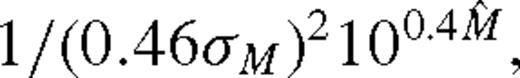
When h_p→h_AUE one might expect the p-method to show the same bias. However, that limit is only approached as σ_π exceeds 0.46σ_M π _p, and assuming π _p≃ π ′ this implies λ > 0.46σ_M. However, this bias is most prominent as λ_u→ 0, so it only appears when σ_M is very small, in which case the bias is vanishingly small.

3 Truncation By Both λ and m with the Direct Method and Variants

The Lutz-Kelker corrections are for magnitudes calculated directly from parallaxes without any weighting. However, we find that sometimes weights are applied to the M′_i, often with h_i =λ⁻²_i. With the method developed by the author (Smith 1987a, Paper III) referred to in S03 as the M-method, the weight has the form

(6)

which (to within a constant in each case) lies between the other two, exactly where depending on the ratio λ_i/σ_M. (This form resembles another choice of weight sometimes used, where the photometric error σ_m is used in the place where σ_m stands.) All these methods may be considered to be ML type fitted to M instead of π ′. Of course the weighting affects the bias, as may be seen in Table 3.

Table 3

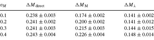
Bias of the direct method and variants with λ-truncation, synthetic data with λ_u = 0.175.

Open in new tabDownload slide

This table has several noteworthy features. First, we see that ΔM_direct and ΔM_λ (the bias with h_i∝λ⁻²_i) do not significantly depend on σ_M, in contrast to the case of the indirect methods (but as is true of the Lutz-Kelker corrections, naturally). ΔM_M does, but only because h_M approaches the constant value 1/σ²_M as σ_M increases and thus ΔM_M→ΔM_direct. Secondly, we note that the uncertainty in ΔM_λ becomes large when σ_M is appreciable, in a fashion reminiscent of that for the AUE method seen in Section 2.3. The reason is probably the inefficiency arising from the omission of σ²_M from the estimated variance. Thirdly, the biases are generally greater than the corresponding ones for the indirect methods.

Suppose that we use the more fashionable cut-off λ_u = 0.1. Table 4 shows how the biases change with that value. Once again they are, with the exception of ΔM_M, virtually independent of σ_M, being approximately 0.27 of their respective previous values. As before, the uncertainty is much greater for ΔM_λ than for the others.

Table 4

Bias of the direct method and variants with λ-truncation, synthetic data with λ_u = 0.1.

Open in new tabDownload slide

For the record, the transformation method developed by Smith & Eichhorn (1996) and improved by Smith (2001) gives essentially the same bias with λ-truncation as the direct method. The reason is that for small values of λ the transformation has virtually no effect; it only becomes important when the error is comparable to, or somewhat greater than, the true parallax π.

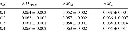
4 Truncation by Both h and m with RP methods

There is some connection between λ and h (in the sense of small h accompanying large λ) but not a simple relation. Because FC truncated their Cepheid sample according to weight, we thought to look briefly at what effect that might have on the results with their method (the FC method). It turns out that h-truncation does not introduce bias with the AUE method or the p-method, as we explain below.

The bias generated by h-truncation with the FC variant of the RP method, calculated numerically, is shown in Table 5 for m_l equal to 9 and 12. It does not seem to vary much for the three cut-offs considered (median, upper quartile and upper decile) or for the choice of m_l, being approximated by −1.3σ²_M. On the other hand, when there is no truncation in h the bias is roughly −0.7σ²_M. Why should there be any bias at all, when as was noted in the Introduction the positive and negative errors ought to cancel out with magnitude-limited samples? There is of course the modelling bias 0.23σ²_M which is common to all three variants of the RP method. As Table 5 shows, however, the total bias with the FC variant is negative. This fact implies that there is some additional source of bias. The other two methods show only the modelling bias when there is no h-truncation (magnitude-limited sample), so the negative bias is unique to the FC method. Furthermore, by implication the bias cannot be due to the m-dependence as discussed in Section 2.4 for λ-truncation because h depends on α⁻² for all three methods.

Table 5

Bias of the FC method with h-truncation, calculated numerically.

Open in new tabDownload slide

This negative bias must originate in the form of the weight h_FC. Because the latter depends upon π ′, it is in principle correlated with the parallax error δ π ′. From equation (4) we see that h_FC is smaller when δ π ′ > 0 and larger when δ π ′ < 0 for any given true parallax π. Consequently there is a negative weighting bias caused by the correlation of h_FC with δ π ′. (In fact the negative bias discussed in Section 2.4 arises from the magnitude dependence of h and thus is another example of this type of bias. The difference is that with the latter the weight is not correlated with the error.) The amount of the weighting bias in this instance appears to be roughly 0.93σ²_M, or four times more than the modelling bias but in the opposite direction. Its magnitude depends on σ_M because σ_M multiplies π ′ (and thus the error δ π ′) on the right-hand side of equation (4).

The bulk of this bias comes from stars with small or negative π ′ as shown in Fig. 5. The cumulative weighted average of the scaled parallax p starting from larger π ′, shown by the filled circles, only becomes negative near the point where π ′= 0, as a result of the numerous relatively large negative errors δp. (A related diagram is fig. 2 of S03.)

Figure 5

Errors in scaled parallax p for a synthetic sample with N = 4000 having M₀ = 10, σ_M = 0.4, σ_π = 30 mas and m_l = 12. The solid curve is the sum of weights σh_FC (multiplied by 10³), and the filled circles are the running average σh_FCp/σh_FC for all parallaxes greater than the given π ′ (multiplied by 10).

Open in new tabDownload slide

The h-truncation itself evidently introduces an additional bias −0.6σ²_M because it does not merely de-emphasize parallaxes with positive errors but excludes some of them. In this sense it resembles λ-truncation but in the opposite direction. With the AUE and p-method variants there is no connection between the parallax error and h, so there is neither a weighting bias nor a truncation bias dependent upon h.

We have not attempted to model the Cepheid sample of Feast & Catchpole for this study. However, based on our present (rather simple) model calculations, it seems likely that because σ_M for those stars (around the period-luminosity, P–L, relation) is almost certainly 0.1 mag or less, the effect of these biases on their results must be negligible, of the order of 0.01 mag at most. The fact that the p-method and grid method gave values virtually identical to those of FC (cf. S03) likewise argues that those authors' results are essentially unaffected by weighting or truncation bias. In other situations where σ_M is larger, the weighting and h-truncation biases would quite possibly be important, considering that both these biases depend on σ²_M.

It has been pointed out by the referee that the amplitude of variation of Cepheids is typically considerably larger than 0.1 mag, and that this variation affects the magnitude limit. On the other hand, the estimation of distance is based upon the averaged apparent magnitude rather than the instantaneous value. For this reason it seems to us that the dispersion around the mean P–L relation is the appropriate σ_M to use. To be sure, some portion of that may be due to uncertainty in the average magnitudes arising from the variability and sampling effects.

5 Discussion

We have shown that use of some indirect ML luminosity calibration methods — the RP method in three forms and the grid method from S03 — with λ-truncated parallax samples that are effectively parallax-limited gives biased results. This fact is not surprising given that the direct method is known to be biased by λ-truncation and the methods used assume a Gaussian distribution for the parallax errors which is not present because of the truncation. There are, however, two noteworthy surprises.

The first is the variety in the amount of bias from λ-truncation with the various methods and weighting schemes considered, including not only the indirect methods but also some of the direct methods. The bias can even be negative rather than positive as a result of a type of bias not considered in S03, namely weighting bias. In particular, the classical Lutz-Kelker corrections are only appropriate with the unweighted direct method and the M-method in the limit of large σ_M. With all the other methods considered here they are invalid.

The second surprise is that the bias with some of the RP methods actually increases in absolute value as λ_u is reduced. Intuitively one would expect the opposite. In the limit σ_M→ 0 that holds true, but not for σ_M≠ 0.

It must be admitted that the cases considered here are somewhat unrealistic, in several respects. Many actual samples are not limited by m_l at all but are selected according to other criteria. The value of m_l itself is often determined by instrumental sensitivity limits or some other external considerations and is fixed. One can vary it, but only to smaller values, at the expense of discarding some data and, in principle at least, some precision. The spatial distribution is usually non-uniform, leading to different numerical values for the bias from those found here. Also, the error values that we have used are quite large compared with those for modern ground-based measurements and the data from Hipparcos. Furthermore, the errors are usually different from one star to another, which modifies the value of m_t. However, our main conclusions ought to remain qualitatively valid despite these objections, at least as long as there is a well-defined m-truncation. A change in σ_π changes the scaling but none of the essentials. It might be desirable to consider m versus m_t for each star individually in more realistic situations.

Let us consider the published studies that have used λ-truncated samples. If the sample in such a study is effectively magnitude-limited there will be no λ-truncation bias, as we noted above. Following up our earlier estimate for the transition magnitude m_t, we crudely estimate the maximum m_l value for a sample to be strictly magnitude-limited as

(7)

where π _λ,max≡σ_π,max/λ_u with σ_π,max being the largest of the {σ_π,i}. If m_l is already given, e.g. by instrumental sensitivity limits, then the mean M₀ must approximately satisfy

(8)

Otherwise the sample will be in the transition regime discussed in Section 2.1 or be parallax-limited and the results will be invalid.

The Hipparcos parallaxes have errors ranging from 0.6 to as much as 3 mas or slightly more (Perryman et al. 1997). The catalogue was compiled using an input catalogue subject to a variety of selection criteria; however, it was considered desirable to add stars so as to render it complete to a fixed limit. The limit is very roughly V≃ 7.5, depending on the stellar type and the galactic latitude (Turon et al. 1992). If a particular type of star has σ_M = 0.1 and λ_u is chosen to be 0.1, we find that for a magnitude-limited sample we should have M₀≳ 5.2. If M₀ is smaller one may arrive at a ‘mean’M which is either larger or smaller than M₀, depending upon σ_M, the method (p-method or grid versus AUE or FC), and the difference between m_l and m_crit,l. Even worse, in cases where one is dealing with a luminosity relation, one portion of it may be magnitude-limited, with no bias but requiring a Malmquist shift if one seeks M₀; another region parallax-limited, with bias and no offset; and there may then be a transitional region between the two having both bias and an offset that varies across the region. The fitting is often done in magnitude space, which means that a direct method is used. For example, the Wilson-Bappu relation based on calcium line emission cores spans a range of at least 11 mag, from M_V about +8 to −3 (Pace, Pasquini & Ortolani 2003). Using Hipparcos data we would expect the lower end to be magnitude-limited and the upper end to be parallax-limited. For the latter region the bias corrections must be modified if the fitting is done with the magnitudes weighted by λ⁻². In this particular situation the problems are exacerbated by a large cosmic scatter, estimated to be 0.6 mag.

To summarize, λ-truncation not only wastes data but also can introduce substantial confusion into luminosity calibrations, especially when its effects on the particular method used are not properly taken into account. For these reasons it should in our opinion generally be avoided. However, if one desires to use such a sample the grid method is readily modified so as to take into account the λ-truncation in forming the likelihood: one simply inserts into the normalizing integral in the denominator of the likelihood (equation 31 in S03) the factor

with π ′_l,i =σ_π,i/λ. This possibility was originally pointed out by Ratnatunga & Casertano (1991, their equation 13) for their ML calibration method, which is basically equivalent to ours of Paper V (with the typos of the latter corrected). None the less, we consider it preferable to use a general ML method like the grid method on a magnitude-limited sample to find M₁ and then, if M₀ is desired, apply the appropriate Malmquist shift. In this way all the data, including negative parallaxes, can be utilized. We are well aware that the Malmquist shift is somewhat problematic because it, like the Lutz-Kelker corrections, depends on the space distribution of the sample. However, we believe that this difficulty can be largely overcome.

Acknowledgments

The author is grateful to the referee, Dr P. Teerikorpi, for suggesting several revisions to make clearer certain points. Also, Dr F. Arenou furnished information on the Hipparcos catalogue which was quite helpful.

References

Appendix

APPENDIX A:

To find the form of the lower envelope for the h–p distribution with the FC method, we can rewrite h_FC,i by substituting λ_ip_i for α_iσ_π,i to get

(A1)

the smallest value of h for given p is for the largest λ, namely λ_u. The form of the envelope is therefore

(A2)

which is 3.94h^−1/2_FC for the particular case shown. For the AUE method the weight can be written just like h_FC for σ_M = 0, or h_AUE = (λp)⁻². Again identifying the lower envelope with λ=λ_u, we have that p_min =λ⁻¹_uh^−1/2_AUE; for the given values this is 5.71h^−1/2_AUE. (The common form and the factor of 1.45 between the coefficients explain why the FC and AUE diagrams look so similar despite the difference in scale.) We obtain the envelope for the p-method by expressing p and h parametrically, as functions of m. Substitution for α_i and π _p,i in terms of m_i and leads to the form

(A3)

if σ_π is the same for all stars, as in our example. We may again write λp =ασ_π, and obviously p_min =ασ_π/λ_u. Solving for p_min, we obtain

(A4)

By inspection the largest possible value of h_p is , which explains the sharp upper bound on h with this method. Substituting, we get

(A5)

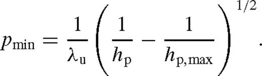
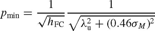
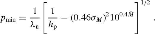
This equation implies that the lower envelope goes to p_min = 0 where h_p =h_p,max. For σ_M = 0.4 and we have h_p,max = 0.0025, which explains the value of the upper bound on h_p in Fig. 2(b). Contrast this behaviour with that of the lower envelopes of the FC and AUE distributions, which only asymptotically approach p_min = 0 as h→∞. As implied by equation (2) and the definition of α_i, h_AUE increases exponentially as m decreases and thus can be quite large as seen in Fig. 2(c), whereas h_p is strictly limited and h_FC also tends to be because of the second term in brackets in equation (3).