Morphological studies of the Spitzer Wide-Area Infrared Extragalactic survey galaxy population in the UGC 10214 Hubble Space Telescope/Advanced Camera for Surveys field Free

Abstract

1 Introduction

A key question on galaxy formation and evolution, in particular about the early-type subpopulation which includes the most massive galaxies at any redshifts, is when and on which time-scales their stellar content has been formed and assembled. Two schematic models are often confronted with the observations: the monolithic collapse model (Eggen, Lynden-Bell & Sandage 1962; Larson 1975; Chiosi & Carraro 2002) and the hierarchical assembly scenario (e.g. White & Rees 1978; White & Frenk 1991; Somerville & Primack 1999; Cole et al. 2000). In the monolithic collapse, a burst of star formation occurred at very high redshifts (z_form= 3) and was followed by passive evolution of the stellar populations, whereas in the hierarchical assembly scenario the time-scales for more massive galaxies are longer, resulting in somewhat younger mean ages. According to the latter interpretation, ellipticals are formed by mergers and/or accretion of smaller galaxies over time-scales comparable to the Hubble time (see, for example, Bell et al. 2004; Faber et al. 2005).

Fundamental observational constraints on the star formation history and the formation pattern are provided by the broad-band colours, line strength indices and stellar chemical abundances. When referred to massive ellipticals, these data suggest that the bulk of stars might have been formed in a remote past. However, some secondary activity of star formation in the recent past is also evident: nearby ellipticals show a large variety of morphological and kinematic peculiarities (e.g. Longhetti et al. 2000) and a substantial spread of stellar ages, particularly for the field population (Thomas et al. 2005). Strong evolution in the population of early-type galaxies has been reported by Kauffmann, Charlot & White (1996) and Kauffmann & Charlot (1998), which has been considered to support the hierarchical galaxy formation models.

The current results about the number counts and redshift distributions of the evolved galaxies at high redshift are still rather inconclusive, and theoretical models about their formation and evolution are correspondingly uncertain (see Somerville et al. 2004, for a brief review).

Near-infrared surveys are best suited for the study of faint high-redshift galaxy populations, for various reasons: the observed fluxes are minimally influenced by K-corrections and only weakly affected by dust extinction, and at the same time good indicators of the stellar mass content of galaxies (Dickinson et al. 2003). Mid-infrared observations, on their side, are strongly informative about phases of active star formation in galaxies (Franceschini et al. 2001; Rowan-Robinson 2001; Xu et al. 2003, and many others). After the Infrared Space Observatory (ISO) exploratory observations, the Spitzer Space Observatory mission has started to map systematically the high-redshift Universe at such long wavelengths.

The main aim of the Spitzer Wide-Area Infrared Extragalactic survey (SWIRE) is the study of the evolution of both actively star-forming and passively evolving galaxies, by exploiting a huge sample of some two million galaxies that are detected within the ~50 deg² of the survey.

Good-quality optical data are essential for the identification and characterization of Spitzer sources. However, typical images obtainable from the ground are not adequate for accurate morphological analysis and source classification. In this paper we exploit very deep multiband public images taken with the Advanced Camera for Surveys (ACS; Ford et al. 1998) in a small portion of the SWIRE N1 field, in order to study the morphological properties of the infrared (IR) emitting galaxies. In what follows and unless specified otherwise, IR refers to 3.6 and 4.5 μm.

In Section 2 we describe the optical (Hubble Space Telescope/ACS) and IR (Spitzer) data used in our analysis. In Section 3.1 we give a brief description of the tools used for the morphological analysis and classification as well as a comparison of their results. In Section 4 we describe a comparison of our modelistic galaxy number counts with our observational data. Finally, in Sections 4.3 and 5 we summarize our results and conclusions.

2 The Data

SWIRE N1 was the first field to be observed by Spitzer for the SWIRE Legacy programme. The IR data used here were obtained in 2004 February and the SWIRE catalogues we use throughout this work were processed by the SWIRE team. Source extraction was performed using sextractor (Bertin & Arnouts 1996) with local background mesh subtraction. Kron and 2.9-arcsec aperture fluxes were used here, for extended and point-like sources, respectively. The Kron fluxes were extracted within a minimum radius of 2 arcsec using a Kron factor of 2.5. These fluxes were the default fluxes in the first SWIRE data release. The 3.6- and 4.5-μm counts are roughly 90 per cent complete at around 10 μJy. The astrometric accuracy is better than 1 arcsec. More details about the entire data set can be found in Lonsdale et al. (2004), Surace et al. (in preparation) and Shupe et al. (in preparation), as well as the data release document (Surace et al. 2005).

The optical data were obtained with the ACS on the Hubble Space Telescope. The field is centred on UGC 10214 (also known as VV 29 and Arp 188, the Tadpole galaxy), a bright spiral at z= 0.032 with a huge tidal tail. The optical catalogue contains some 5700 objects with 10s detection limits for point sources of of 27.8, 27.6 and 27.2 AB magnitudes in the g_F475W, V_F606W and I_F814W bands, respectively. For details on the data reduction and catalogue production, see Benitez et al. (2004). This field lies close to the centre of the SWIRE N1 field, providing an unprecedented opportunity of combining very deep optical data with high-quality IR data in wavelength ranges so far poorly explored.

Within the ~14 arcmin² ACS field, we use an area of ‘10 arcmin² well outside the region occupied by the UGC 10214 galaxy. Any remaining background contamination likely to affect the Infrared Array Camera (IRAC) fluxes is accounted for thanks to the way the SWIRE catalogues are created: they use a locally generated background estimate and any underlying faint extended emission is considered as background and subtracted.

The matching between the SWIRE and ACS sources was done using the tmatch task of iraf, with a 1-arcsec match radius. The sources were then visualized one by one and a flag was assigned to each one of them, stating their status with respect to close counterparts. Out of the 177 matched objects, 175 and 130 are detected in 3.6 and 4.5 μm, respectively (with two having only 4.5-μm detections) and 18 (i.e. ~10 per cent) have at least two extracted ACS counterparts within a 1-arcsec radius. For six of them, however, we can clearly identify the object that mostly contributes to the IRAC fluxes, as the difference in I-band magnitude between the counterparts is larger than 2.5. For a detailed discussion of the optical/IR bandmerged catalogues and the spectral energy distribution (SED) of the matched objects, we defer to Pérez-Fournon et al. (in preparation) and Hernán-Caballero et al. (in preparation).

The I-band counts for the entire ACS field and for the sources with a SWIRE counterpart are shown in Fig. 1 by solid and dashed lines, respectively. Down to a magnitude of I~ 22.5 almost all ACS sources have an IR counterpart, while the number starts dropping below I~ 23.5, reflecting the shallowness of the SWIRE data. The completeness of the 3.6-μm counts drops quickly below 10 μJy, value corresponding to an AB limiting magnitude of 21.4 or I~ 23.5 for a typical I-3.6 μm colour of 2 (see Fig. 2 for the colour distribution of the 177 matched sources).

Note that the probability of chance associations within 1 arcsec of radius is less than 2 per cent up to an I-band magnitude of 24.0 and up to 5 per cent at an I-band magnitude of 25. Taking into account the I-band magnitude distribution of the SWIRE sources (Fig. 1), one expects fewer than five out of the 177 sources to be wrongly matched.

3 Morphological Classification

3.1 Tools for the morphological analysis

A number of parametric and non-parametric methods are suggested in the literature for quantitative assessment of the morphological properties of intermediate- and high-redshift galaxies. Among the parametric approaches, an often used representation of the galaxy morphological types is the Sérsic index, n, which appears in the surface brightness profile law , where I_b(0) is the bulge central intensity, r_m is the bulge semimajor effective radius and n is the Sérsic shape parameter (Sérsic 1968). The quantity b_n is a function of n, and is chosen so that r_m encloses half of the total luminosity. The Sérsic profile includes the classical de Vaucouleurs profile when n is equal to 4.

Figure 1.

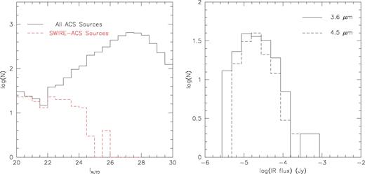
Left panel: I-band number counts for all ACS sources (solid line) and for the SWIRE—ACS identifications (dashed line) in the ~10 arcmin² field covered by the ACS observations, after the area around UGC 10214 has been removed. Right panel: 3.6-μm (solid line) and 4.5-μm (dashed line) distributions of the SWIRE-ACS sources.

Open in new tabDownload slide

Figure 2.

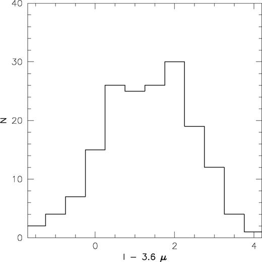
(I-3.6 μm)_AB colour histogram for the matched SWIRE—ACS sources.

Open in new tabDownload slide

Alternatively, non-parametric approaches have been proposed, with the most common one using the combination of the light concentration (C), asymmetry (A) and clumpinesS (S), or CAS, parameters. Concentration (Abraham et al. 1996) roughly correlates with the Sérsic index, while asymmetry (Conselice, Bershady & Jangren 2000) compares the image of a source with its rotated (usually by 180°) counterpart, enabling the distinction between normal and irregular galaxies or merging systems. The clumpiness (Conselice 2003) measures the uniformity of the light distribution in a galaxy. Abraham et al. (1996) and later on (Conselice et al. 2000) showed that bulge-dominated, disc-dominated and merging systems occupy different but often overlapping regions in the asymmetry—concentration space. Conselice (2003) finally demonstrated that all galaxy types can be roughly identified by their position in the CAS three-dimensional space.

Our morphological analysis has been performed in three independent steps: (i) visual inspection, in order to attribute each object to a given morphological class based on features such as the presence of spiral arms and/or bars, signs of interaction, multiple nuclei etc; (ii) a non-parametric analysis of the galaxy light distribution using the CAS parameters (see Conselice et al. 2003 for a detailed description and Cassata et al. 2005 for their exact definition as used here); (iii) a detailed analysis of the surface brightness profiles using the packages galfit (Peng et al. 2000) and gasphot (Pignatelli, Fasano & Cassata 2005).

3.2 Results of the morphological analysis

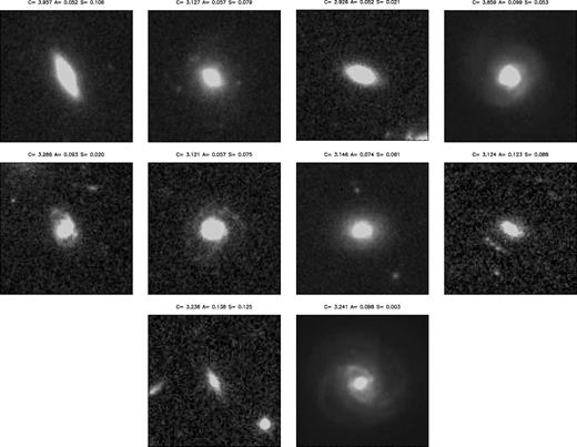
In the 10.56 arcmin² region of the ACS field uncontaminated by UGC 10214, there are 177 objects with a SWIRE counterpart. As a first step, a visual inspection of these sources was carried out on the I-band image by three of the authors, independently. The individual results were then compared and finally combined after the very few dubious cases were discussed (the excellent quality of the ACS data allows for very little doubt about the morphological characteristics of the objects at these relatively bright magnitudes). The visual analysis has identified four main groups of objects — spheroids (consisting of ellipticals and S0 galaxies), spirals, irregular galaxies and pairs — and found four objects too faint to be classified: 21 were stars (stars were double-checked adopting the criterion of Benitez et al. 2004 for stellar classification, i.e. a sextractor class_star= 0.94); 37 spheroids; 69 spiral galaxies; 24 irregulars; and 22 merger or interacting systems or sources with multiple components (all characterized as pairs). Fig. 3 shows examples of each of the categories along with their CAS parameters, discussed hereafter.

Figure 3.

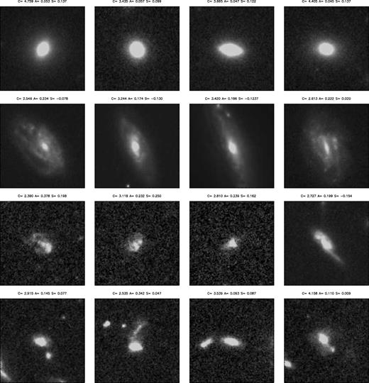
Examples of objects visually classified as ellipticals, spirals, irregulars and pairs (from upper to lower row) and their CAS parameters. The size of the cutouts is 5 × 5 arcsec².

Open in new tabDownload slide

For nearly a quarter of the 156 galaxies (the 21 stars are from now on excluded), CAS parameters were not computed. Before computing CAS, pixels below 2× RMS are filtered out (corresponding to 25 mag arcsec⁻²). For objects with no pixels above this level, A and S are not computed. The computation of C makes use of the sextractor-derived growth curve of each object and no filter is applied on the image. For objects with complex structure (visually classified as pairs or irregular galaxies), their multiple components or uncommon shape render the CAS analysis difficult. For the rest of the sources, however, this approach gave results largely in agreement with the visual inspection. Spheroids tend to have lower A and higher C than spirals, irregulars or pairs and tend to concentrate around S~ 0.1. In fact, 36 of the 37 visually classified spheroids lie in or at the very borders of the region shown in Fig. 4, defined by

(1)

(2)

(3)

Figure 4.

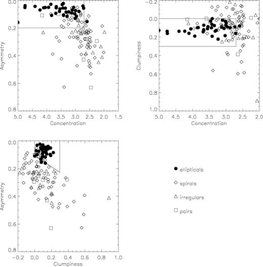
Asymmetry, concentration and clumpiness for the SWIRE-ACS galaxies and comparison with the classification obtained by visual inspection.

Open in new tabDownload slide

An additional set of 10 objects falls within this same region. These objects are spirals but at least seven of them have prominent bulge components, as seen on the cutouts illustrated in Fig. 5. Note that for some of them it is difficult to see the spiral arms or disc components on the cutouts due to the chosen contrast, but they are clear enough on the actual image for the objects to be classified as spirals. We therefore deduce that more than 93 per cent of the objects in the designated area of the CAS parameter space are ellipticals or bulge-dominated spirals (lower limit if one considers the 36 ellipticals and the seven clearly bulge-dominated spirals among the 46 objects lying in this area).

Figure 5.

The 10 galaxies visually classified as spirals that lie in the CAS spheroid region.

Open in new tabDownload slide

This analysis sets the lower and upper limits of the number of spheroids in 37 (visually classified) and 46 (included in the region delineated by equations 1–3), respectively, within the ~10 arcmin² of effective area of the UGC 10214 ACS field.

The results of the parametric methods are more difficult to interpret. For low-asymmetry objects, the results of galfit and gasphot are in reasonable agreement with each other (Fig. 6) but discrepancies arise for the objects with A > 0.25. This is somewhat expected as the less symmetric galaxies cannot be easily reproduced by parametric models that are intrinsically symmetric (see Cassata et al. 2005 and Pignatelli et al. 2005 for further details on the comparison between gasphot and galfit on real and simulated galaxies, respectively). Some 80 per cent of the objects have Δn/n less than 0.5, the region indicated by the dashed lines in Fig. 6. Note that for some of the objects the two codes failed to converge and therefore do not appear on this plot (31 for galfit and 25 for gasphot, with 20 objects in common between the two failing groups). Parametric and non-parametric approaches also agree up to a point, with the Sérsic index, n, correlating with C in the majority of the cases (Fig. 7). Some 15 sources, however, present large deviations. For these objects, the errors on the estimated values of n are very large due to their nature: they are all pairs, sources with multiple components or (just one case) objects with very small isophotal area.

Figure 6.

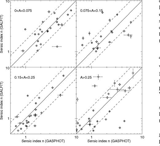
Sérsic index, n, computed by galfit versus n computed by gasphot for the SWIRE-ACS galaxies, in bins of asymmetry. The two tools provide comparable results for low-asymmetry objects. The dashed lines mark the region where , occupied by ~80 per cent of the objects. Objects with n < 0.5–22 in total — or objects for which one of the methods did not converge — are not shown.

Open in new tabDownload slide

Figure 7.

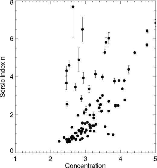
Sérsic index, n, computed by galfit versus concentration, C. n scales with C in the majority of cases. The objects with the largest scatter are also those with the largest error bars and, in the majority of cases, have been visually classified as pairs (including systems with various components).

Open in new tabDownload slide

The distribution of Sérsic index, n, given by galfit is roughly bimodal, culminating at a value around 1 for late-type and around 2 for early-type galaxies. However, one-third of the galaxies visually classified as early types have an n lower than 2, and about the same fraction of late-type galaxies have n greater than 2, implying that using a classification criterion based on the Sérsic index alone (see, for example, Ravindranath et al. 2004) would result in a certain amount of misclassifications. Among the early-type galaxies with a low value of the Sérsic index, a large fraction are S0 galaxies while a certain number have a too small isophotal area to obtain reliable fits of the surface brightness distribution. Finally, the largest part of late-type galaxies having large Sérsic indices is mostly composed by bulge-dominated systems or again objects occupying too small isophotal areas. Note that there was no lower limit imposed on the isophotal area in order to perform the fits; however, all objects for which the fit failed to converge consisted of less than 50 pixels.

The entire morphological analysis may be subject to an, unaccounted for, morphological K-correction. Morphological classification performed at a given band suffers from this effect as galaxies of higher redshifts are actually observed at bluer rest-frame wavelengths (Windhorst et al. 2002; Papovich et al. 2003; Cassata et al. 2005). Windhorst et al. (2002) found that the morphology of galaxies changes when moving from the optical to the ultraviolet passbands. However, our analysis should not be much affected by this effect as we do not expect a large number of high-redshift galaxies, due both to the relatively bright fluxes and to the very small size of the field. This, in fact, somewhat ensures that we study galaxies with rest frame between B and I bands. In particular, the number of high-redshift spheroids, the population we are mostly interested in, must be particularly low. Rowan-Robinson et al. (2005), based on photometric redshift estimations and model predictions, showed that no more than 25 per cent of the 3.6-μm galaxy sample down to a limit of 10 μJy have redshifts larger than ‘1, the largest fraction of which are late-type objects. CAS analysis may also suffer from the effects of the morphological K-correction (see, for example, Conselice et al. 2000; Lotz, Primack & Madau 2004) as, in general, moving toward shorter wavelengths results in larger values of A and S and smaller C. However, because we have ignored the real redshifts of our objects and decided not to rely upon the photometric redshifts provided by Benitez et al. (2004)— calculated based on three optical passbands only — in order to avoid introducing further uncertainties, we have chosen not to apply any kind of correction.

Finally, the effects of the aperture on the estimation of the CAS parameters have not been considered here. The parameter most sensitive to the size of the aperture is A (Conselice et al. 2000) and is more likely to be affected in the case of faint, high-redshift objects. However, because much of our analysis is based on the C parameter and because the vast majority of our objects have very bright ACS counterparts (see Fig. 1, left panel), we are confident that aperture effects do not bias our work. The fact that visual inspection and CAS analysis are in such good agreement when selecting early-type objects is also in support of our argument.

4 Galaxy Number Counts

4.1 Observed number counts

The IRAC1 and IRAC2 channel (3.6 and 4.5 μm) observed cumulative galaxy counts are reported in the left column of Fig. 8. The various morphological classes are those derived from the visual inspection. We now confine our analysis to fluxes brighter than 10 μJy in the two bands, and assume that the sample is 90 per cent complete here. This flux-limited sample consists of a total of 109 galaxies, among which 28 are spheroids.

Figure 8.

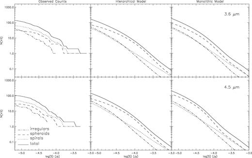
Left column: observed cumulative 3.6-μm (upper panel) and 4.5-μm (lower panel) counts for the various types of objects (as classified by visual inspection) and their total number (solid line). Middle and right columns: cumulative model counts for the hierarchical (middle) and monolothic (right) models. The counts are reported here for the various different morphological classes as indicated in the line caption. Note that monolithic and hierarchical scenarios only differ in the spheroid (and therefore also total) counts.

Open in new tabDownload slide

It is interesting to note here that the IRAC channels 1 and 2 are optimally suited for the identification and analysis of spheroidal galaxy populations. We have performed an automated analysis of the I-band images over the entire ACS field using the CAS parameter set and found that only ‘7 per cent of the galaxies to the survey limit I= 27.2 lie in the area defined by equations (1)–(3), and are therefore classifiable as spheroids. The same analysis performed on the counterparts of the SWIRE IRAC population shows a much larger incidence (‘20 per cent) of early-type galaxies. This is the result of the IR selection, favouring the detection of galaxies with old stellar populations. Deeper SWIRE observations might reveal later-type IR counterparts of the ACS sources; however, this is not evident from the actual distribution of morphologies of the IRAC sources with the I-band magnitude. The percentage of early-type objects in bins of magnitude in the interval [19.0, 25.0] takes values between 15 and 45 per cent but without demonstrating any specific trend.

4.2 Model number counts

We now compare the statistical observables derived from our Spitzer IRAC data set with simple evolutionary models. While the details on the models are more extensively described in Franceschini et al. (in preparation), we provide here a summary of our general approach. We adopt in the following H₀= 70, Ω_M= 0.3 and Ω_Λ= 0.7.

In our approach, four main galaxy classes are considered: spheroids, quiescent spirals, an evolving population of irregular/merger systems (hereafter starburst population), and minor contributions from active galactic nuclei.

The SED templates describing the spectral shapes at different galactic ages, needed to calculate the K-corrections, have been computed using the stellar population synthesis code grasil (Silva et al. 1998). We adopt a Salpeter initial mass function (IMF) with a lower limit M_l= 0.15 M_⊙ and a Schmidt-type law for the star formation rate: Ψ(t) =νM_g(t), where ν is the efficiency and M_g(t) is the residual mass of gas. A further relevant parameter is the time-scale t_infall for the infall of primordial gas. The evolution patterns for the models considered here are obtained with the following choices of the parameters: for early-types, t_infall= 1 Gyr, ν= 1.3 Gyr⁻¹; for late-types, t_infall= 4 Gyr, ν= 0.6 Gyr⁻¹. The corresponding star formation law for ellipticals has a maximum at a galactic age of 1.4 Gyr, and is truncated at 3 Gyr to mimic the onset of a galactic wind. For late-type galaxies, the peak of the star formation occurs at 3 Gyr. The parameters assumed to reproduce the spectra of spirals and irregular galaxies are those of a typical Sb spiral. This may not be very representative of an evolving population during a starburst phase; however, given the spectral region considered in this work, our assumption is still a good approximation. We have then generated two grids of model SEDs for both early and late types, spanning a range of ages from 0.1 to 15 Gyr. For what concerns the spheroids, we made the assumption that these stellar systems are gas- and dust-free, so that extinction is negligible. Extinction is instead considered for late-type galaxies, with an evolution of the dust to gas ratio typical of an Sb galaxy (we assume the parameters proposed by Silva et al. 1998). Heated dust possibly contributes to the emission from the late-type galaxies at rest-frame wavelengths longer than 2–3 μm, which could affect the derived model flux densities in the IRAC bands. This will be considered in a future work.

For the local luminosity function we have made use of that estimated by Kochanek et al. (2001) for both early-type and late-type galaxy classes and derived from a K-band selected sample taken from the Two-Micron All Sky Survey (2MASS), including 4192 low-redshift (z‘ 0.02) galaxies.

Our schematic model for both the spheroidal and the spiral populations assumes that the galaxy comoving number density remains constant once the population is formed at a given redshift, while the galaxy luminosities evolve following their evolutionary stellar content.

On the other hand, the analysis of deep galaxy surveys in the K band (Cassata et al. 2005; Franceschini et al., in preparation) indicates the presence of a numerous population of irregular/merging systems at high redshifts, likely requiring luminosity as well as density evolution going back in cosmic time. We then add a population of starbursts whose density ρ(z) evolves with the following rule

(4)

for z < 1, and constant above, and whose luminosity L(z) increases as

(5)

for z < 2, and constant above.

Before detailing the comparison of our model predictions with the observed statistics derived from our sample, we need to consider how a morphological selection correlates with a classification based on the intrinsic SED of galaxies. A convenient way to directly check this point is to look at the colours of the SED templates assumed by the model, in order to verify if they are representative of the morphologically selected spheroids and spiral populations.

As an example, in Fig. 9 we report the I-4.5 μm versus the g-3.6 μm observed colour-colour plot, compared with the evolutionary tracks derived using model templates. The blue dots mark the visually classified late-type sources; the red open circles are spheroids; the green triangles are galaxy pairs. The curves show the evolutionary tracks corresponding to elliptical and spiral SEDs at different ages (thick red solid, dotted and dashed lines denote ellipticals of 1, 2 and 10 Gyr, respectively; blue solid, dotted, dashed and long-dashed lines denote 3, 5, 10 and 15 Gyr, respectively), spanning the redshift range between 0 and 1.8. Fig. 9 suggests that morphologically selected elliptical galaxies preferentially populate the reddest region of the observed colour distribution. However, the colour degeneracy between age and extinction prevents us from having an unambiguous photometric selection for spheroids. This can also be seen in this figure, where spheroids and late-type galaxies occupy contiguous and partially overlapping regions of the colour-colour space. The above-mentioned degeneracy between age and extinction have thus produced star-forming sources with observed red colours (generally attributed to old stellar systems). Similarly, those spheroids that have undergone recent episodes of star formation have bluer colours and then fall within the region preferentially populated by late types.

Figure 9.

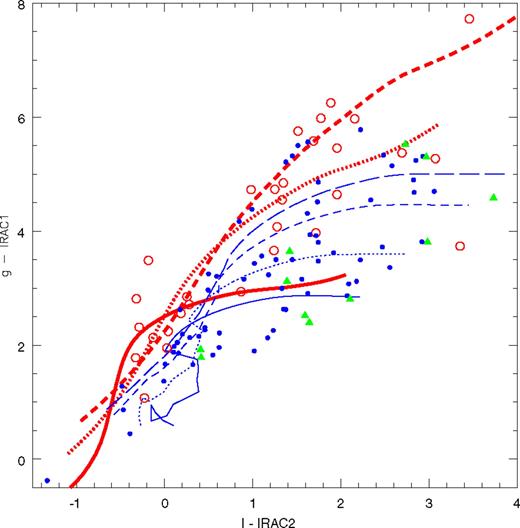
Colour-colour diagram (g-IRAC1) versus (I-IRAC2) showing the location of the spheroids, spirals and pairs (open circles, dots and filled triangles, respectively) and the model evolutionary tracks of ellipticals and spirals of various ages (thick red and thin blue lines, respectively; for details about the line coding, see text).

Open in new tabDownload slide

This analysis suggests that a pure morphological selection is not obviously comparable with a colour criterion, and that a given amount of contamination affects such a comparison. However, assuming that the template SEDs discussed above are reasonably representative of the morphological classes, we have investigated the statistical properties of the SWIRE sample and compared them with the model predictions. Any conclusion based on this analysis has to be taken with caution, in particular for the specific properties of the different spheroidal and spiral/irregular classes.

We now explore two schemes for the formation of spheroidal galaxies. The first corresponds to the classic — monolithic — scenario assuming a single impulsive episode for the formation/assembly of the field ellipticals, occurring at a high redshift (z_form > 2.5; e.g. Daddi, Cimatti & Renzini 2000; Cimatti et al. 2002). In our current implementation, we assume a redshift of formation z_form= 3.0. In this single burst model, the birth of the stellar populations is coeval to the formation of the spheroids.

The second model for spheroidal galaxies — the hierarchical model — describes a situation in which massive ellipticals form at lower redshifts through the merging of smaller units down to recent epochs. In such a case, the formation of early-type galaxies is spread in cosmic time. Very schematically, we achieve this by splitting the local spheroidal galaxies into several subpopulations, each forming at different redshifts (in coincidence with the birth of a new population of stars building up the younger spheroids). All subpopulations have the same mass function but different normalizations, whose total at z= 0 has to reproduce the local luminosity function. This model is being tested against deep galaxy surveys in the K band, showing a general tight agreement between predictions for the different morphological classes and observations: K20 (Cimatti et al. 2002); HDFS (Franceschini et al. 1998; Rodighiero, Franceschini & Fasano 2001); GDDS (Abraham et al. 2004). In our current implementation, the bulk (‘60 per cent) of the early-type mass function is dynamically assembled in the redshift interval 1.1 < z < 1.6, with additional fractions being assembled at higher and lower z. At this stage, and for simplicity, we do not consider extinction effects during the star formation phase of the spheroids. We defer to Franceschini et al. (in preparation) for a more detailed discussion and additional applications of this modelling.

Fig. 8 shows the predicted cumulative number counts for the hierarchical (middle panel) and monolithic (right panel) scenarios, respectively. The difference is essentially in the spheroidal population. The main value of these models is to provide, particularly for the spheroidal and normal spiral components, the simplest possible extrapolations of the local luminosity functions back in cosmic time. The addition of a strongly evolving population of irregular/mergers is instead motivated by the need to reproduce, at least at the zeroth order, the observed statistics from deep K-band counts (Franceschini et al., in preparation). In any case, these simple models predict that spheroidal galaxies would make important contributions to the Spitzer/IRAC counts at fluxes above 10 μJy.

4.3 Discussion

We report in Figs 10 and 11 detailed comparisons, with model expectations, of the SWIRE observed integral counts at 3.6 and 4.5 μm for the various morphological classes in the Tadpole ACS image. Only a general distinction between spheroidal and non-spheroidal systems is made here, the latter including both spirals and irregulars/mergers. The observed counts are shown down to 10 μJy, roughly the 90 per cent completeness limits of the SWIRE IRAC1 band. The solid and dashed lines correspond to the hierarchical and monolithic scenarios, respectively, while the dotted lines show the observed number counts. More precisely, the two dotted lines appearing in these figures for each morphological class correspond to the lower and upper boundaries on the source real density, which have been discussed in Section 3.2. The upper and lower limits in this case of spheroids correspond to the CAS analysis and visual inspection, respectively, whereas in the case of the remaining classes (marked in the plot as ‘other’) the upper limit is due to visual inspection and the lower to the CAS parameters. The observed IRAC1 counts given by Fazio et al. (2004) are shown for comparison (marked as diamonds in Figs 10 and 11). Note that, given the modest statistics of our source sample, the detailed shapes of the counts (showing bumps and humps at the bright end of the counts) are not to be considered as significant.

Figure 10.

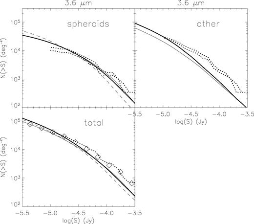
Comparison of the observed (dotted line) and model (solid and long-dashed lines for the hierarchical and monolithic scenarios, respectively) 3.6-μm number counts. The upper and lower limits for the observed counts are given by the CAS parameter analysis and visual inspection, respectively, as discussed in the text. Note that, compared with Fig. 8, the spiral and irregular galaxies are here combined in the ‘other’ class. The diamonds in the lower panel represent the IRAC1 counts given by Fazio et al. (2004). The dashed-triple-dot line shows the predictions of an improved version of the model presented in Xu et al. (2003) (see text for details).

Open in new tabDownload slide

Figure 11.

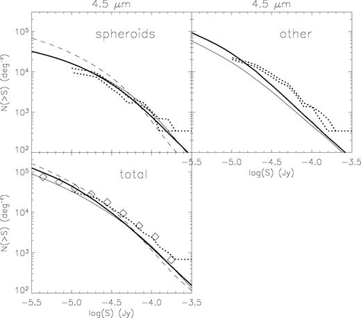
Same as Fig. 10 but for 4.5 μm.

Open in new tabDownload slide

Despite the very small size of our sample, the total counts are in good agreement with those observed by Fazio et al. (2004) over a much larger area (several deg²), especially the 3.6-μm counts. In the case of the 4.5-μm counts, the statistics start being really poor as we are dealing with only 104 objects detected in this band down to the adopted flux limit. The observed spheroidal counts are in very good agreement with those predicted by the hierarchical scenario while the monolithic model suggests steeper counts. However, while the models predict counts essentially dominated by ellipticals (see middle and right panels of Fig. 8), we observe an excess of late-type galaxies and merger-irregulars to dominate the counts. Comparison between this same model and K-band observations did not show any discrepancy.

The observed spheroid counts are inconsistent with the monolithic predictions that imply too steep number counts and would not only exceed the observed counts at the faint fluxes but also underpredict the bright end 3.6-μm counts. A coeval origin for spheroids at high redshift (i.e. formation of their stars in an instantaneous burst at z > 3) therefore seems to produce excess counts compared to observations. Changing the stellar IMF during the star formation phase from a Salpeter to, for example, a Scalo (1986) distribution would probably somehow ease the inconsistency (Cimatti et al. 2002), but at the cost of not explaining by large factors the extragalactic background radiation intensities (Madau & Pozzetti 2000; Franceschini et al. 2001) and the observed metallicities of intracluster plasmas (Mushotzky & Loewenstein 1997).

On the other hand, the observed numbers of spiral and irregular galaxies are larger than predicted by our simple evolutionary scheme. This simple model, consistently fitting the K-band galaxy statistics, falls short of the observed counts at both 3.6 and 4.5 μm. The rising of the contribution of the late-type population to the 3.6- and 4.5-μm emission, with respect to its contribution at 2.2 μm, might suggest a much stronger evolution (in both density and luminosity) for star-forming galaxies at longer wavelengths. Our results might indicate that the 3.6-μm band selects more active galaxies than the K band (2.2 μm). If in the model the starburst and spiral populations are then assumed to contribute more significantly to the source counts, the discrepancy with observations should be reduced. Moreover, a more suited set of SED templates describing the star-forming population should be included — accounting for polycyclic aromatic hydrocarbon (PAH) emission and a more accurate description of dust and extinction, given that in our approach we roughly assume similar spectra for spirals and evolving starburst. However, larger sample and statistics are needed to check this assumption.

Very qualitatively, it might be tempting to interpret the observed excess population of irregulars and mergers and their inferred strong cosmological evolution as the progenitors of spheroidal galaxies, the rapid relaxation and gas exhaustion following the merger bringing a sudden appearance of a spheroid. Obviously, any more quantitative conclusion will require much further information on source identifications and redshifts.

Because of the inconsistency between observed and model late-type galaxies, we further compared our results with an improved version of the model presented by Xu et al. (2003). In its original version this model overpredicted the 24-μm counts at flux levels of ‘1 mJy (for a detailed discussion, see Papovich et al. 2004 and Shupe et al. in preparation). In order to correct for this effect but still fit the 15-μm ISO counts, the evolution rate of starburst galaxies was lowered with respect to the old model and the strength of the PAH features in the wavelength range of 5 < λ < 12 μ m was raised by a factor of 2 in the SEDs of both starburst and normal galaxies. Thus, the predicted late-type counts are still below the observed limits but are higher by a factor of ~1.5 than those predicted by our simple hierarchical scenario. They are shown in dashed-triple-dot line in Figs 10 and 11. This reinforces our previous statement about the deficit of model late-type galaxies reflecting the lack of PAH emission from the models presented in Section 4.2.

5 Conclusions

In this paper we have presented the results of a morphological analysis of a small subset of the SWIRE galaxy population. Our sample is flux-limited at 3.6 and 4.5 μm and consists of 156 galaxies. Our analysis is based on public ACS data taken inside the SWIRE N1 field. We distinguish two very general classes of galaxies, bulge- and disc-dominated galaxies, the first class being referred to with the general term ‘spheroids’ and the second containing everything from spirals to irregulars and pairs. Even though the requirement for 3.6- and/or 4.5-μm detections favours the selection of early-type galaxies, the sample under study is dominated by a large fraction of disc galaxies and interacting systems (~80 per cent), already suggesting that elliptical galaxies assemble late.

The monolithic and hierarchical models checked against this data set considerably underpredict the number of late-type galaxies. The observed 3.6- and 4.5-μm early-type counts are in very good agreement with the estimations of the hierarchical scenario, showing however a deficit toward the fainter end of the counts, possibly reflecting some incompleteness that is already introduced at this flux level. The monolithic predictions imply steeper counts and fail in reproducing the observations. The disagreement is stronger at the faint end of the 4.5-μm early-type counts.

An additional comparison of the data set with another model available in the literature (Xu et al. 2003) suggested that dealing in an appropriate way with some of the model deficiencies such as the dust or PAH emission components should result in a better agreement. It should be mentioned that the model predictions may depend significantly on the assumed stellar IMF (see, for example, Cimatti et al. 2002), although the one we adopted here should be rather representative of the main phases of star formation. The model itself is rough and the predicted counts should not be taken at face value but rather be considered indicative of the expected tendencies.

This ACS data set is the deepest available, as of today, in any of the SWIRE fields, and therefore the results of the present analysis are of great importance for the understanding of the SWIRE galaxy population. Due to the small size of our sample, however, we cannot be very conclusive and can only outline some general tendencies. We would like to point out a number of potential sources of uncertainty in the interpretation of our results: (i) the way that large-scale structure may influence the results, given the particularly small size of the ACS field; (ii) the possible existence of heavily obscured, by dust, ellipticals at the stage of their formation; (iii) the assumption of a priori values instead of a χ² minimization on some of the model parameters; and finally (iv) the uncertainties on the exact shape of the SEDs of the various galaxy types in these newly explored, IR wavelengths.

Acknowledgments

This work is based on observations made with the Spitzer Space Telescope, which is operated by the Jet Propulsion Laboratory, California Institute of Technology under National Aeronautics and Space Administration (NASA) contract 1407. Support for this work, part of the Spitzer Space Telescope Legacy Science Program, was provided by NASA through an award issued by the Jet Propulsion Laboratory, California Institute of Technology under NASA contract 1407.

ACS was developed under NASA contract NAS 5-32865, and this research has been supported by NASA grant NAG5-7697. We are grateful for an equipment grant from Sun Microsystems, Inc. The Space Telescope Science Institute is operated by AURA Inc., under NASA contract NAS5-26555.

This work was supported in part by the Spanish Ministerio de Ciencia y Tecnologia (Grants No. PB1998-0409-C02-01 and ESP2002-03716) and by the EC network ‘POE’ (Grant No. HPRN-CT-2000-00138).

We would like to thank N. Benitez for making publicly available the reduced ACS image used in this work.

Finally, we thank the anonymous referee for the precise and detailed report that greatly improved the presentation of our work.

References