William Herschel Telescope observations of distant comets Free

Abstract

Introduction

Comets are the remnants of the original accretion disc of our Solar system and preserve, to various degrees, the conditions that existed during its formation. Understanding the physical, compositional and dynamical properties of these bodies is crucial if we are to understand how our Solar system formed, its subsequent evolution, and how it is likely to evolve in the future. Furthermore, if we are to assess accurately the possible consequences of a collision with Earth, we must first obtain an abundance of physical data on these objects.

Direct observations of cometary nuclei are difficult owing to the presence of active cometary comae at small heliocentric distances. Conversely, when the nuclei are far from the Sun and apparently inactive, they are too faint to be observed. However, modern CCD cameras mounted on large telescopes have the ability to image faint nuclei at large heliocentric distances (typically >3 au), where the coma contribution is small or negligible, yielding an estimate of the brightness of the bare nucleus. Another technique which is particularly effective utilizes coma subtraction methods on Hubble Space Telescope observations (Lamy, Toth & Weaver 1998). Resolved images of a cometary nucleus have been obtained in only three cases, those of 1P/Halley by the Giotto and Vega spacecraft, 19P/Borrelly by the Deep Space 1 probe, and most recently comet 81P/Wild 2 by Stardust.

Less than 37 per cent of the known population of Jupiter-family comets have had their radii reliably estimated to date (Lamy et al. 2004), and only about one-quarter of those have had their albedos constrained. Also, there is considerable disagreement regarding the slope of the cumulative size distribution for the Jupiter-family comet population, as determined from a combination of past observations (Fernández et al. 1999) versus more recent CCD surveys (Lowry, Fitzsimmons & Collander-Brown 2003; Lamy et al. 2004; Meech, Hainaut & Marsden 2004). A least-squares fit to the Fernández et al. data set, for those comets with perihelion distances <2 au, gives a cumulative radius distribution that can be fitted by a power law of the form N(≥r) ∝r^−α, where α= 2.65 ± 0.25. For the more recent published CCD surveys, values for α range from 1.59 to 1.90 for the observed size distributions. The close agreement amongst the latter surveys indicates that we are indeed converging on a robust solution. It is interesting to note the similarity of the slope of the Jupiter-family size distribution to that of the near-Earth asteroids for which α= 1.75–1.95 (Rabinowitz et al. 2000; Stuart 2001; Bottke et al. 2002). More intriguing is the large difference from the Kuiper Belt Object (KBO) population for which α= 3.2–4.2 (Gladman et al. 2001; Larsen et al. 2001; Trujillo et al. 2001). Clearly, this difference implies that the current KBO size distribution estimates cannot be reliably extrapolated down to small sizes (i.e. a broken power law exists), or that major evolutionary changes are occurring on minor bodies as they evolve inwards toward the inner Solar system.

This study is part of an on-going programme to obtain ‘snap-shot’ observations for a large sample of Jupiter-family comets. Observations of this kind provide no rotational or shape information, but have the advantage that a large number of comets can be observed on any given night. This is particularly beneficial for building a data base from which to select suitable targets for future detailed study. For those comets that display little or no activity at large heliocentric distances, we can use the previously determined effective radius measurements to assess the expected signal-to-noise ratio levels of planned observations, rather than ‘shooting blind’ which is obviously not an efficient use of precious large-telescope time. Conversely, those comets that display substantial coma activity are important for studies of distant activity for which very little is known in the region beyond 3 au from the Sun (Szabo et al. 2001).

Single colour measurements for a wide sample of cometary nuclei are also valuable, not only for detailed planning of future observations, but for understanding the overall distribution of surface properties. Of course, full rotational-phase coverage of the nucleus is ideal, but any colour variation is expected to be small (Campins, A'Hearn & McFadden 1987; A'Hearn et al. 1989) and thus single colour measurements should be close to the global averages. Also, it has been successfully demonstrated that combining published photometry from multiple observers can be used to constrain nucleus properties such as the phase coefficient (Fernández et al. 2003). Many comets have been observed under this ‘snap-shot’ scheme (Licandro et al. 2000; Lowry et al. 2003; Lowry & Weissman 2003a; Meech et al. 2004), and we are now at the point where we can begin to constrain the nucleus size distribution reliably, and to pick and choose which comets are most suitable for more detailed studies.

In this paper we describe the analysis of ‘snap-shot’ observations of distant comets taken with the 4.2-m William Herschel Telescope in 2002 July. The structure of this paper is as follows. Section 2 describes the observations, the instrumental set-up and the photometric calibration procedure. Section 3 describes the analysis of the surface brightness profiles of each comet, which was carried out to assess the degree of coma activity. In Section 4 we discuss the effective nucleus radius measurements obtained from the photometry, and in Section 5 we discuss the colour measurements obtained and compare with published data. Finally, a brief summary is provided in Section 6.

Observations

Snap-shot observations of several comets were performed on the nights of 2002 July 12/13 and 13/14 using the 4.2-m William Herschel Telescope (WHT) on the island of La Palma (Spain). The instrument used was the Prime Focus Imaging Camera which comprises an optical mosaic of two EEV 2k × 4k CCDs. The pixel scale is 0.24 arcsec pixel⁻¹, and the total field of view is 16.2 × 16.2 arcmin². The gap between the two chips is 9 arcsec, and both chips were used in unbinned mode. Owing to the alt-azimuth design of the telescope, the imaging camera is placed on a rotating table so that the northern direction is parallel with the y-axis of the CCD chips. The telescope pointing was re-initialized to a clean portion near the centre of CCD2, as this chip had many fewer hot pixels and defective columns than its counterpart. Therefore only image frames from CCD2 were used in the subsequent analysis. Standard Harris R and V broad-band filters were used, which have central wavelengths at 640.8 and 543.7 nm, respectively.

Sky conditions appeared photometric throughout the entire observing run, which was later confirmed through analysis of standard star fields that were obtained alongside the object exposures. Multiple exposures of the Stetson photometric standard field NGC 6341 were taken throughout the night for photometric calibration. As a consistency check, a single image of the Landolt standard field PG 2331+055 (Landolt 1992) was obtained and its instrumental magnitude extracted using aperture photometry. After conversion to apparent magnitude via the transformation equations derived from the Stetson standards, it was found that the apparent magnitudes of the stars within the PG 2331+055 field differed from the true Landolt values by less than 0.01 mag in R and less than 0.04 mag in V. Therefore it is reasonable to state that any resulting cometary magnitudes are in the Landolt photometric system, which is itself based on the Johnson and Kron–Cousins systems.

Pre-processing of the object images included flat-fielding using images of the twilight sky and bias subtraction. A fringe pattern was evident on the R-band images, which was removed in the standard manner using a fringe map constructed by combining multiple long-exposure R-band images. A total of 11 comets were targeted, from which seven were successfully detected. These comets are 43P/Wolf–Harrington, 129P/Shoemaker–Levy 3, 133P/Elst–Pizarro, 143P/Kowal–Mrkos, 149P/Mueller 4, P/1998 U4 (Spahr) and P/2001 H5 (NEAT). Unfortunately, comet 149P/Mueller 4 was removed from the analysis as it was merged with a background star and no reliable photometry could be obtained. Comet images were obtained with the telescope tracking at the apparent rate of motion of the comet, and so the detected comets typically appeared as near-azimuthally symmetric entities, and the background stars were trailed. As a final check that we did indeed detect the comet, we compared the actual position of the comet with the predicted position. Stars from the United States Naval Observatory A2 star catalogue were used for the astrometry. For those comets that remained undetected, it was found from astrometry that their predicted position fell on or very near relatively bright background stars. Therefore we were unable to measure brightness upper limits for these comets.

The observational geometry of each comet is presented in Table 1, along with an image log. The heliocentric distances range from a minimum of 2.81 au for comet 133P/Elst–Pizarro to a huge 6.12 au for comet P/1998 U4 (Spahr). Not all comets in our sample have previously measured phase coefficients, but those comets that didn't were observed at phase angles below 10°, and so uncertainties in absolute magnitude or size due to unknown phase darkening coefficients are small. Comet exposure times were fixed at 900s across both filters, and the airmass of observation was kept below 1.7 to minimize the effects of atmospheric extinction on the calibrated magnitudes. Notice that more comets were observed on the first night of observation, due to a camera malfunction during the first half of night 2.

Table 1

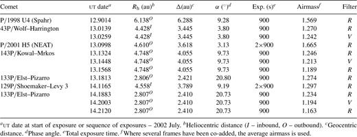
Observational log.

Open in new tabDownload slide

Surface Brightness Profiles

In order to search for visible signs of activity, we compared the radial surface brightness profiles (SBPs) of each comet with our best estimate of the background point spread function (PSF). Unfortunately, on this occasion the non-sidereal tracking of the WHT was less than optimal. The trails of background stars were distorted in a manner consistent with a slight instability in the differential tracking, which resulted in a shifting of the PSF perpendicular to the expected direction of the trail. This effect was compounded by a small trail-curving effect caused by the rotation of the detector during the exposure. As discussed in Section 2, on an alt-azimuth telescope, rotation of the detector during exposures keeps the north–south direction aligned with the y-axis of the CCD images.

To reconstruct the background PSF for a given frame, we first selected a bright, well-isolated background star. The section of the image containing the background star was copied and saved as a separate image in order to simplify the subsequent analysis. The trimmed image was rotated so that the trail direction was aligned with the x-axis of the image. The rows were collapsed along the trail to give the one-dimensional brightness profile of the star perpendicular to the trail direction. The length of the collapsed region was defined by the apparent motion of the comet. Take the V-filter image of 133P/Elst–Pizarro, taken on 2002 July 13, as an example. In a 900-s exposure the comet would had moved 5.31 arcsec across the CCD from its predicted rate of motion at the time of the observations. Therefore the collapsed region was 5.31 arcsec long and its centre coincided with the estimated centre of the trail. Finally, the sky background was subtracted using a sampling region 10 pixel wide on either side of the trail. This method provides the effective brightness profile that would have been obtained under sidereal tracking.

For comets with two co-added images, namely comets P/2001 H5 (NEAT), 143P/Kowal–Mrkos, 129P/Shoemaker–Levy 3 and 133P/Elst–Pizarro (July 12), the method needed to be slightly different because of a gap in the stellar trails on the co-added image caused by a time delay between the end of one exposure and the start of the next. We take the co-added R-filter image of 133P/Elst–Pizarro obtained on 2002 July 13 as an example (the total exposure time is 2 × 900 s). First, the image sections containing a background star from each of the individual frames were rotated, aligned and co-added. Then, the profile was extracted from this co-added section in the normal way. However, the length of the collapsed region is defined by the trail length in a 900-s exposure, rather than the length of the trail in an 1800-s continuous exposure.

This procedure was performed for each comet and the resulting 1D brightness profiles were calibrated and scaled to the brightness of the comet. Both cometary and stellar profiles were converted to mag arcsec⁻² versus projected cometocentric distance ρ (arcsec), and the plots are shown in Figs 1(a)–(f) for comets with R-filter images, and Figs 2(a)–(c) for comets with V-filter images. This method was quite successful in reconstructing the untrailed PSF, as demonstrated by the close agreement between the brightness profiles of comets 133P/Elst–Pizarro, 143P/Kowal–Mrkos and P/2001 H5 (NEAT) and the scaled PSFs of their respective background stars. Comets 129P/Shoemaker–Levy 3 and P/1998 U4 (Spahr) have brightness profiles that are more diffuse than their respective PSFs, indicating an active state. Comet 43P/Wolf–Harrington is a special case due to a tracking error during the exposure, causing the comet to appear smeared on the R-filter CCD image as shown in Fig. 3(a). The diffuseness of its brightness profile as indicated in Fig. 1(a) may lead to a false conclusion that this comet is visibly active. Fortunately, the telescope tracking was optimal during the V-filter exposure (see Fig. 3b). The SBP of the comet in the V-filter image was extracted and its active nature was unambiguously confirmed as illustrated in Fig. 2(a). A faint tail is also visible on the V-filter image. V-filter SBPs were also extracted for comets 133P/Elst–Pizarro and 143P/Kowal–Mrkos as an additional check on their apparent stellar appearance. In both cases the V-filter SBPs match those of their respective scaled PSFs. We considered only the second nights' images for the brightness profile analysis of comet 133P/Elst–Pizarro, owing to poor tracking on the first nights' images.

Figure 1

Azimuthally averaged SBPs from R-filter images. Solid circles signify the cometary brightness (mag arcsec⁻²) at various distances from the central pixel of the comet, and the open triangles signify the integrated R magnitude as measured through a circular aperture of radius ρ arcsec. The solid curve represents the scaled PSF for the frame, the vertical lines represent the radii of photometric apertures used in the apparent magnitude measurements, and the labelled horizontal dashed lines denote the measured apparent magnitude. Comets 133P/Elst–Pizarro, 143P/Kowal–Mrkos, and P/2001 H5 (NEAT) appear unresolved, whereas comets 43P/Wolf–Harrington, 129P/Shoemaker–Levy 3 and P/1998 U4 (Spahr) appear to be active.

Open in new tabDownload slide

Figure 2

Azimuthally averaged surface brightness profiles of comets with V-filter images. Quantities represented by symbols and lines are the same as in Fig. 1. The telescope tracking for the 43P/Wolf–Harrington image was superior to that of its R-filter counterpart. The V-filter brightness profile is unambiguously more diffuse than the background PSF, indicating an active nucleus. Comets 133P/Elst–Pizarro and 143P/Kowal–Mrkos display a stellar-like appearance, consistent with their R-filter images.

Open in new tabDownload slide

Figure 3

R- and V-filter CCD images of the active and unresolved comets. The telescope tracking in the R-filter 43P/Wolf–Harrington image is quite poor compared with its V-filter image, although a faint tail is seen extending towards the lower left quadrant on both images. Comets 129P/Shoemaker–Levy 3 and P/1998 U4 (Spahr) are also active, and the remaining comets are stellar in appearance.

Open in new tabDownload slide

For the active comets we describe the SBP in terms of the SBP gradient m defined as

1

where F(ρ) is the observed flux at ρ and m =−1 for the steady-state case. Within such a steady-state coma model the observed brightness decreases as 1/ρ, and the volume density of the isotropically emitted dust grains N_d∝ 1/ρ². Profile gradients with −1.5 ≤m < −1 are most likely due to radiation pressure acting on the dust grains, while m < −1.5 indicates the presence of sublimating grains. In Figs 1 and 2 we overplot two diagonal lines representing the m =−1 and m =−1.5 cases for those comets whose SBPs indicate activity. We find that the active comets in our sample are adequately described by simple radial outflow models, perhaps subject to slight radiation pressure effects. This is quite typical for comets observed at large heliocentric distances (Szabo et al. 2001; Lowry et al. 1999).

Effective Radii and Dust Production

Aperture photometry was performed on each comet to measure their respective apparent magnitudes. For each comet, instrumental magnitudes were measured through a series of apertures extending from the central brightness peak out to just beyond the point where the surface brightness of the comet became indistinguishable from the background sky. The resulting apparent magnitudes plotted as a function of aperture radius (or cometocentric distance) are shown in Figs 1 and 2 for the R and V filters respectively (open triangles). The apertures used for the apparent magnitude measurement were limited to the radial extent of the detectable SBPs. In other words, the aperture radius was taken to be the point where the SBPs start to blend with the background sky. This point is indicated by a vertical line on each of the plots of Figs 1 and 2. From these plots, one can see that the apparent magnitudes remain constant beyond the vertical line, at least within the photometric uncertainties. Although the chosen apertures are slightly less than the canonical 3× FWHM, we find that the aperture correction (out to 3× FWHM) amounts to no greater than 0.79 per cent of the total cometary flux and thus is considered negligible. These calculations were performed for the unresolved comets only, and the aperture corrections were obtained using the reconstructed background stellar profiles discussed in Section 3.

These apparent magnitudes were converted to effective radii using the usual formula

2

where A_λ is the geometric albedo in the R or V filter, r_N (m) is the effective radius of the nucleus, R_h (au) and Δ(au) are the heliocentric and geocentric distances, respectively, and α and β are the phase angle and phase coefficient, respectively. M_⊙ is the apparent R or V magnitude of the Sun. We use solar apparent magnitudes of −27.26 and −26.9 for the R and V filters, respectively. In all cases we assume a geometric albedo of 0.04 and a phase coefficient of 0.035 mag deg⁻¹ (Lamy et al. 2005), with the exception of comets 133P/Elst–Pizarro and 143P/Kowal–Mrkos for which phase coefficients of 0.044 ± 0.007 and 0.043 ± 0.014 mag deg⁻¹ were recently measured (Hsieh et al. 2004; Jewitt et al. 2003). The derived effective radius estimates for the unresolved comets range from 1.02 ± 0.05 to 4.56 ± 0.12 km. Upper limits for the active comets range from 1.94 ± 0.12 to 4.15 ± 0.20 km. Table 2 lists the individual values along with their respective apparent magnitudes. Comets 43P/Wolf–Harrington, 143P/Kowal–Mrkos and 133P/Elst–Pizarro have R and V measurements. In all three cases the resulting effective radii across both filters are consistent at the 2σ level.

Table 2

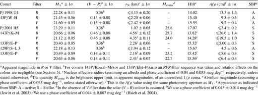
Broad-band photometry, nucleus effective radii and Af_ρ values.

Open in new tabDownload slide

For the unresolved comets, we estimated what the unresolved coma magnitude should be if one were present. We take the simple case of a steady-state coma model the observed brightness of which decreases as 1/ρ, as discussed above. Following Jewitt & Danielson (1984), the unresolved coma magnitude M_coma measured within a circular aperture of radius ρ (arcsec) is obtained from the following relation:

3

where B(ρ) (mag arcsec⁻²) is the measured surface brightness at ρ through the R or V filter. We can measure an upper limit for B(ρ) from the SBPs presented in Figs 1 and 2. The vertical lines in these figures represent the radius of the photometric aperture used for the apparent magnitude measurements. As discussed above, this indicates the point at which the SBP blends with background sky and so the cometary SBP is essentially undetectable at this point. Taking the surface brightness at this point as a suitable limit for B(ρ) (indicated by open circles in Figs 1 and 2), we calculate the respective M_coma values which are listed in Table 2. Comparing these M_coma values with their respective apparent magnitudes, we find that the brightnesses of the potential unresolved comae constitute no more than 8.2 per cent for comet 133P/Elst–Pizarro, only 1.0 per cent for comet 143P/Kowal–Mrkos, and 12.2 per cent for comet P/2001 H5 (NEAT). Note that for comets 133P/Elst–Pizarro and 143P/Kowal–Mrkos we consider R-filter M_coma values only even though V-filter M_coma values were obtained. This is because the difference between M_coma and M_λ is greatest for the R-filter images. The estimated coma/nucleus flux ratios are all very low, which implies one of two possible scenarios for each of the stellar-like comets. Either there exists a tightly bound unresolved coma for which the surface brightness falls off much more steeply than the canonical 1/ρ, or the activity levels are low and the nucleus dominates the observed flux measurement by an amount indicated by the above percentages. More specifically, the contribution of the nucleus to the observed flux would be >91.8 per cent for comet 133P/Elst–Pizarro, >99.0 per cent for comet 143P/Kowal–Mrkos, and >87.8 per cent for comet P/2001 H5 (NEAT).

Comet 43P/Wolf–Harrington has been previously observed on multiple occasions. Lowry et al. (1999) report observations obtained in 1995 when the comet was at an inbound heliocentric distance of 4.87 au. The effective radius was 3.3 ± 0.7 km. Lowry et al. (2003) returned to the comet again in 1999 when the comet was at an outbound heliocentric distance of 4.46 au. The resulting effective radius was 3.4 ± 0.2 km, totally consistent with the previous measurement. On both occasions the comet appeared stellar, but it should be noted that a 1-m telescope was used. Licandro et al. (2000) obtained V-filter measurements in 1992 when the comet was at an outbound heliocentric distance of 3.04 au. In order to compare their photometry with ours, we converted their V-filter apparent magnitude to an R-filter apparent magnitude using the (V–R) colour index obtained here of 0.15 ± 0.08, and assumed an albedo and phase coefficient of 0.04 and 0.035 mag deg⁻¹, respectively. Their effective radius comes out as 2.37 ± 0.11 km. Activity was observed by Licandro et al. and hence this is an upper limit. This is close to the upper limit reported here of ≤2.2 ± 0.06 km. The brightness of the projected nucleus cross-section during our current observations – whether in the presence of a coma or not - obviously cannot exceed the measured total brightness. As our brightness upper limit is fainter than the previous brightness measurement of Lowry et al. (2003), we can then place reasonable constraints on the nucleus shape. The full range of observed R-filter absolute magnitudes is 0.97 ± 0.15, which implies a minimum axial ratio a/b of 2.44:1 using a/b≥ 10^0.4Δm, where Δm is the full absolute magnitude range. We add a note of caution to this conclusion, in that it depends heavily on whether or not coma activity can be entirely ruled out in the Lowry et al. (2003) observations even though no resolvable coma was observed. Furthermore, if a coma were present and contributed significantly to the measured flux during the Lowry et al. (2003) observations, then why is the comet so much more intrinsically fainter here even though the comet was at a comparable heliocentric distance? This discrepancy is consistent with a rotating elongated nucleus dominating the observed flux during the previous Lowry et al. observations (barring the usual possibility of an outburst). These facts constitute reasonable evidence that if a coma was present on 43P/Wolf–Harrington during the previous Lowry et al. observations then its contribution was most likely small or negligible.

Comet 143P/Kowal–Mrkos was recently observed in 2001 June–November when the comet was at an outbound heliocentric distance of 3.4–4.0 au (Jewitt et al. 2003). Time-series R-filter magnitudes were measured to reveal a double-peaked synodic rotation period of 17.21 ± 0.10 h. Jewitt et al. found an effective nucleus radius of 5.7 ± 0.6 km, but used their best-fitting Bowell-type phase law (Bowell et al. 1989) having G = 0.15 to extrapolate down to α= 0°. Taking their mid-June data, and using a linear phase coefficient of 0.043 ± 0.014 mag deg⁻¹ (in order to be comparable with our data), we estimate that their mean R-filter apparent magnitude corresponds to an effective radius of ∼4.98 ± 0.07 km. Their photometric range was found to be Δm = 0.45 ± 0.05 mag, therefore the corresponding effective radii range from ∼4.49 ± 0.06 to 5.53 ± 0.08 km. Our radius measurement of 4.56 ± 0.12 km falls within this range. Given that the Jewitt et al. measurements were performed at 1.35 au closer to the Sun just 1 year prior to our observations, and that our estimated coma flux is ≤1 per cent, we can safely say that this comet was caught in an inactive state.

Comet 133P/Elst–Pizarro was previously observed between 2002 August and December, at heliocentric distances of 2.62–3.27 au (Hsieh et al. 2004). Hsieh et al. found a mean absolute R-band magnitude of 15.61 ± 0.01 using their measured linear phase coefficient of 0.044 ± 0.007 mag deg⁻¹. This agrees extremely well with our absolute R-band magnitudes of 15.51 and 15.61 when the full magnitude range of 0.4 magnitudes from Hsieh et al. is taken into account.

We measured the relative dust production levels for the active comets using the Afρ formalism (A'Hearn et al. 1984). This quantity does not give the actual mass-loss rates, but rather a means to compare dust production levels at different epochs and from different observers. When measuring the Afρ values we used the same aperture sizes as those used for the apparent magnitudes. We find that the Afρ values are generally low for the active comets and range from 4.5 ± 0.6 to 13.3 ± 1.3 cm. We also placed upper limits on the stellar comets, and those range from 2.4 ± 0.2 to 26.6 ± 1.4 cm. The full list is given Table 2. Although in theory the Afρ quantity is not supposed to vary with aperture size, in practice the quantity will increase slightly with decreasing aperture size. We looked at how Afρ varies inwards from the chosen aperture size to aperture sizes ∼1× FWHM (of the background PSF) and find that the value increases by 31 per cent for P/1998 U4 (Spahr), 55 per cent for 43P/Wolf–Harrington (R-filter), 69 per cent for 43P/Wolf–Harrington (V-filter) and 42 per cent for 129P/Shoemaker–Levy 3.

Colour and Spectral Gradient

As shown in the previous section, the coma contribution to our reported apparent magnitudes is small or negligible for comets 133P/Elst–Pizarro and 143P/Kowal–Mrkos. Colour measurements would likely represent that of the nucleus surface. When measuring cometary nucleus colours, one must be careful not to introduce additional uncertainties due to rotation of an elongated nucleus. As the time between the R and V images of each of these comets was not insignificant, the colour measurements were performed in the following way. First, notice in Table 1 that for comets 133P/Elst–Pizarro and 143P/Kowal–Mrkos we took one V-filter image bracketed by two R-filter images. For each comet, the mid-point ut of the two R-filter images coincides – to within a few tens of seconds – with the ut of the corresponding V-filter image. When we co-added the two R-filter images, the effective ut of the co-added image is essentially the same as the V-filter ut. As colours were obtained by co-adding the two R-filter images, then measuring the apparent magnitude in the co-added frame and simply subtracting it from the corresponding V-filter apparent magnitude, nucleus rotation effects are removed from the colour determination. Comet 43P/Wolf–Harrington is a different case as we only have one R and one V, but the comet was active and so this is not an issue as the nucleus signal is most likely swamped by the coma.

For comets 133P/Elst–Pizarro and 143P/Kowal–Mrkos, previous (V–R) colour measurements have been obtained by other investigators. Those values are 0.42 ± 0.03 (Hsieh et al. 2004) and 0.58 ± 0.02 (Jewitt et al. 2003) for comets 133P/Elst–Pizarro and 143P/Kowal–Mrkos, respectively. Our colour value of 0.46 ± 0.08 for comet 143P/Kowal–Mrkos is consistent at the 1.3σ level with the previous measurement, but the colours for 133P/Elst–Pizarro differ considerably despite the larger error bars on our measurement. Possible explanations for this discrepancy are discussed below.

As noted in the Comets II review (Lamy et al. 2005), there is just a handful of comets for which nucleus (B–V) and (V–R) colour index values exist. However, the sample of comets that have just (V–R) measurements is much larger. As also noted by Lamy et al., several comets have published spectra and are characterized by their normalized reflectivity gradient. In order to successfully inter-compare our (V–R) values with the complete sample, we chose to convert all colours to reflectivity gradient. Broad-band colour indices are related to the normalized reflectivity gradient of the comet S[per cent/100 nm] via the expression

4

where (V−R)_⊙ is the colour index of the Sun, and Δλ is the difference between the central wavelengths of the V and R filters in units of 100 nm. In this case Δλ= 0.97. See Hainaut & Delsanti (2002) for an extended discussion of spectral gradient. In Fig. 4 we plot the ‘cumulative sample percentage’ as a function of spectral gradient for all comets, with the spectral gradients for comets 133P/Elst–Pizarro and 143P/Kowal–Mrkos clearly marked. For those comets for which multiple (V–R) measurements are listed by Lamy et al., we take the average value. One can see from Fig. 4 that the majority of comets have reflectivity gradients in the 0–13 per cent/100 nm region. Comet 143P/Kowal–Mrkos lies within this region and is therefore considered typical in terms of spectral reflectivity. As with comet 143P/Kowal–Mrkos, we find that any possible coma signal for comet 133P/Elst–Pizarro is likely to be small or negligible, and hence that the measured spectral gradient represents that of the nucleus.

Figure 4

Cumulative spectral gradient distribution of cometary nuclei. Most of the spectral gradients are derived from their (V–R) colour indices (Lamy et al. 2005). The positions of comets 133P/Elst–Pizarro and 143P/Kowal–Mrkos are marked.

Open in new tabDownload slide

The measured spectral gradient of 133P/Elst–Pizarro is −19.0 ± 8.2 per cent/100 nm and is amongst the bluest yet measured for a cometary nucleus. This blue colour may indicate a surface with peculiar properties. Until recently this object was thought to be an inactive extinct comet, but recent observations have cast doubt on this hypothesis. Hsieh et al. (2004) have recently monitored the evolution of its dust trail over several months in 2002 and found that the trail structure and brightness changed, indicating that the trail is actively generated over time. As noted by Hsieh et al., this is consistent with the collision theory (Toth 2000), but the most likely cause of the dust release is drag forces from sublimation of surface ices.

Perhaps there is a single icy patch on the surface that happened to be in view during our observations, thus leading to very blue colours. Indeed, this icy patch may just have been recently exposed, leading to the observed dust trail and subsequent fading reported by Hsieh et al. As the trail fades and some of the larger dust particles return to the surface to re-form the dust mantle, the nucleus colours will inevitably redden with time. This may explain why our colours are much bluer than those reported by Hsieh et al., as our observations took place just one month before their observation interval. Such time-scales for mantle formation are possible (Rickman, Fernandez & Gustafson 1990). Furthermore, the Hsieh et al. colours do not show temporal variability indicating surface homogeneity, although the temporal spacing of colours is sparse. We therefore propose that the event that occurred on the surface of 133P/Elst–Pizarro that led to the evolving dust trail of 2002 happened just prior to our observations in 2002 July. Perhaps such an event is periodic, as discussed by Rickman et al. Additional high temporal resolution colour index measurements would be extremely valuable to help answer this intriguing question. One caveat to the icy patch scenario is that there is likely to be a lot more coma contribution to our observed flux than our 1/ρ model suggests. Without more extensive data, further investigation is not possible. Finally, our observations also reveal the presence of the dust trail, and a more in-depth analysis will appear in a future paper.

In Fig. 5 we compare our (V–R) values with those of other comets as listed in the Comets II review (Lamy et al. 2005). The colour indices of comets 133P/Elst–Pizarro and 143P/Kowal–Mrkos are indicated by vertical bars as the (B–V) values are currently unconstrained by our data set. With the exception of comet 45P/Honda–Mrkos–Pajdusakova and one measurement for comet 6P/d'Arrest, most comets lie in a thin diagonal band in BVR colour space and are redder than their equivalent solar colours. One can obtain a rough approximation for what the (B–V) colours are likely to be for our three observed comets by the intersection of the vertical bars with the mid-point of this ‘band’. Slope G₁ represents a linear least-squares fit to the colour measurements, ignoring the two outliers. Slope G₂ represents the colour–colour relationship for a constant spectral gradient across BVR wavelengths. Notice that slope G₂ is somewhat shallower than slope G₁, indicating that the reddest comets tend to have curved spectra, i.e. they get progressively bluer towards shorter wavelengths. Non-linear spectra – over BVR wavelengths – have been observed for several Centaurs and KBOs (Hainaut & Delsanti 2002), suspected progenitors of the majority of the Jupiter-family cometary population.

Figure 5

Colour–colour plots for cometary nuclei from data compiled in the Comets II review (Lamy et al. 2005) and additional data from (Hsieh et al. 2004) (133P/Elst–Pizarro) and (Lowry & Weissman 2003b) (2P/Encke). Only those comets for which (V–R) and (B–V) measurements exist are included. As our data do not include B-filter measurements, our (V–R) colours are indicated by vertical dashed lines. Equivalent solar colours are also marked. Slope G₁ represents a linear least-squares fit to the colour measurements, ignoring the two outliers. Slope G₂ represents the colour–colour relationship for a constant spectral gradient across BVR wavelengths.

Open in new tabDownload slide

Summary

We have analysed data from broad-band V- and R-filter observations obtained at the 4.2-m William Herschel Telescope on La Palma on 2002 July 12–14. A total of six comets were imaged and their heliocentric distances ranged from 2.8 to 6.1 au. Comets observed were 43P/Wolf–Harrington, 129P/Shoemaker–Levy 3, 133P/Elst–Pizarro, 143P/Kowal–Mrkos, P/1998 U4 (Spahr) and P/2001 H5 (NEAT). Our main findings are as follows.

• (i)

  A detailed surface brightness profile analysis indicates that three of the targeted comets were visibly active (43P/Wolf–Harrington, 129P/Shoemaker–Levy 3 and P/1998 U4), and the remaining three comets were stellar in appearance. We find that the active comets in our sample are adequately described by simple radial outflow models perhaps subject to slight radiation pressure effects (−1.5 ≤m < −1), which is quite typical for comets observed at large heliocentric distances.

• (ii)

  Further analysis shows that for the three ‘stellar-like’ comets the possible coma contribution to the observed flux does not exceed 12.2 per cent, and in the case of comet 143P/Kowal–Mrkos the coma contribution is expected to be as low as 1 per cent, and so the resulting photometry most likely represents that of the projected nucleus surface.

• (iii)

  Apparent R- and V- filter magnitudes were measured using aperture photometry that led to effective radii measurements, which for the inactive comets range from 1.02 to 4.56 km. Corresponding effective radius upper limits for the active comets range from 1.94 to 4.15 km. We assumed an albedo and phase coefficient of 0.04 and 0.035 mag deg⁻¹, respectively, except for comets 133P/Elst–Pizarro and 143P/Kowal–Mrkos where the phase coefficients have been previously measured. These values are compared with previous measurements, and for comet 43P/Wolf–Harrington we find that the nucleus axial ratio a/b could be as large as 2.44. For the active comets we find that the Afρ values are generally low and range from 4.5 ± 0.6 to 13.3 ± 1.3 cm. We also placed upper limits on the stellar comets and those range from 2.4 ± 0.2 to 26.6 ± 1.4 cm.

• (iv)

  Spectral gradients were extracted for two of the inactive comets from their measured broad-band colour indices, and compared with the rest of the comet population for which (V–R) colour values exist. We find a spectral gradient for 143P/Kowal–Mrkos of S = 9.9 ± 8.1 per cent/100 nm, which is very typical of Jupiter-family comets the majority of which have reflectivity gradients in the 0–13 per cent/100 nm range. The spectral gradient that we measure for comet 133P/Elst–Pizarro is amongst the bluest yet measured for a cometary body [S =−19.0 ± 8.2 per cent/100 nm].

• (v)

  We have looked at all previous BVR colour measurements for cometary nuclei and we see that for the reddest objects the colour distribution is not consistent with linear spectra over BVR wavelengths. Such curved spectra have also been observed for Centaurs and Kuiper Belt objects (Hainaut & Delsanti 2002).

• (vi)

  We measure a (V–R) colour index of 0.14 ± 0.11 for the nucleus of 133P/Elst–Pizarro, which is considerably lower than previous measurements (Hsieh et al. 2004). As our observations took place just one month before their observation interval, we propose that the event that occurred on the surface of 133P/Elst–Pizarro that led to the evolving dust trail of Hsieh et al. may have happened just prior to our observations in 2002 July. This event may have formed an icy patch on the nucleus surface which reddened as a result of a rapidly formed dust mantle. Finally, our observations also reveal the presence of the dust trail of 133P/Elst–Pizarro.

Acknowledgments

We thank Carrie Trundle for her assistance with the WHT observations, and the referee Javier Licandro for helpful comments. The William Hershel Telescope is operated on the island of La Palma by the Isaac Newton Group in the Spanish Observatorio del Roque de los Muchachos of the Instituto de Astrofísica de Canarias. All image processing, photometry and calibration were performed using the iraf program (Tody 1986, 1993). iraf is distributed by the National Optical Astronomy Observatories, which is operated by the Association of Universities for Research in Astronomy, Inc. (AURA) under cooperative agreement with the National Science Foundation.

References

Footnotes