


Abstract
We have carried out a systematic study of the properties of the kHz quasi-periodic oscillations (QPOs) observed in the X-ray emission of the neutron star low-mass X-ray binary 4U 1608−52, using archival data obtained with the Rossi X-ray Timing Explorer. We have investigated the quality factor, Q, of the oscillations (defined as the ratio, ν/Δν, of the frequency ν of the QPO peak to its full width at half-maximum Δν). In order to minimize the effect of long-term frequency drifts, power spectra were computed over the shortest times permitted by the data statistics. We show that the high Q of ∼200 reported previously for the lower-frequency kHz QPO is by no means exceptional, as we observe a mean Q value in excess of 150 in 14 out of the 21 observations analysed and Q can remain above 200 for thousands of seconds. The frequency of the QPO varies over the wide range 560–890 Hz and we find a systematic trend for the coherence time of the QPO, estimated as τ=Q/(πν) = 1/(πΔν), to increase with ν, up to a maximum level at ∼800 Hz, beyond which it appears to decrease, at frequencies where the QPO weakens. There is a more complex relationship between τ and the QPO rms amplitude, in which positive and negative correlations can be found. A higher-frequency QPO, revealed by correcting for the frequency drift of the 560–890 Hz one, has a much lower Q (∼10) which does not follow the same pattern. We discuss these results in the framework of competing QPO models and we show that those involving clumps orbiting within or above the accretion disc are ruled out.
1 Introduction
Fourier analysis reveals the X-ray emission of low-mass X-ray binaries (LMXBs) to be variable on short time-scales, often with several characteristic quasi-periodic oscillation (QPO) peaks identified between ∼1 Hz and ∼1 kHz (van der Klis 1989, 2000, 2004). The highest-frequency QPOs, reaching up to ∼1300 Hz and usually occurring in pairs, are of particular interest, as their periods correspond to the dynamical time-scale in the inner accretion disc, where strong-field effects of gravity are crucially important. There is no agreement as to the physical origin of the QPOs (van der Klis 2004). In the wealth of observational papers published on QPOs, many have studied the QPO properties as a function of count rate, luminosity, spectra, lower-frequency features and so on, but very few have focused on the coherence time, which is in fact a very constraining parameter for QPO models. In this paper, we study the previously reported kHz QPOs in the X-ray burster, 4U 1608−52, with the aim of characterizing the quality factor, and hence coherence time, of its QPO over a wide range of frequency. We have selected this source for two main reasons. First, its QPOs are known to be strong, and secondly, in the QPO discovery paper of Berger et al. (1996), a quality factor Q=ν/Δν of up to ∼200 was reported for the QPO, together with apparent correlations between its frequency and both its amplitude and width.
2 Data Analysis and Results
We have retrieved the 1996 and 1998 data of 4U 1608−52 from the Rossi X-ray Timing Explorer (RXTE) archive. These data have already been discussed in Berger et al. (1996) and Méndez et al. (1998a,b, 1999). The 1996 data were recorded during the decline of an X-ray outburst, whereas the 1998 data sampled a whole outburst phase from the source. Here, we have restricted the analysis to the ‘science event’ unbinned data. We have thus excluded the 1996 March 6 data, which were obtained in a binned data mode with no spectral information. As the sensitivity for QPO detection increases with the number of photons detected, we have selected only those observations in which the five RXTE proportional counter array (PCA) units were operating (Bradt, Rothschild & Swank 1993). This represents more than 250 ks of data. The data set is divided into 21 segments recorded within different, sometimes consecutive, orbital revolutions of the satellite.
We have computed Leahy normalized Fourier power density spectra (PDS) between 1 and 2048 Hz over 1-s intervals (1-Hz resolution), using X-ray photons of energy between 2 and 40 keV. It is well known that the QPO frequency can vary by as much as 50 Hz in a few thousand seconds. The goal of our analysis is to estimate Q, while keeping the contribution of the frequency shifts as small as possible. This implies that the QPO profile properties have to be estimated on the shortest possible time-scales. For 4U 1608−52, which shows strong QPOs, this can usually be done with 32 s. So we have averaged 32 1-s PDS and searched for a QPO peak using a sliding window algorithm, as described in Boirin et al. (2000). In segment 11, where the QPO is the weakest, we have averaged 128 1-s PDS. We have preferred to use 32 summed 1-Hz spectra rather than a single power spectrum obtained over, say, 32 s, as in this way we can make a direct comparison with the results discussed below (Section 2.2), which rely on having 1-s time resolution. Using 32-s spectra would formally give better frequency resolution, but we have found that the reduction in the measured widths and the improvement in the uncertainties in the parameters are very small.
To obtain reliable fits, only features of significance larger than 6σ are considered, although decreasing this threshold to 5σ does not affect the results. In our data set, QPOs are detected on 1996 March 3 and between 1998 March 24 and 29 (see Fig. 1 and Table 1).

Time-evolution of the 560–890 Hz lower-frequency QPO detected from 4U 1608−52 over the whole data set. The image is a dynamical power density spectrum, in which each column is a PDS integrated over 32 s. The x-axis shows the sequence number. The QPO corresponds to the boldest parts of the image. Note that for the longest segment of 1996 March 25 (segment 11) the QPO is barely visible in the image.

Mean Q factor of the low-frequency kHz QPO observed from 4U 1608—52 in the 21 segments of data. The count rate is given in cts s−1 in the 2–40 keV range for the five PCA units. Nint is the number of 1-s PDS averaged. Ns is the number of averaged PDS. Nd is the number of PDS in which the QPO was detected above the 6σ threshold. νmin,max are the minimum and maximum QPO frequencies measured in the 32-s PDS. The rms is the root mean square amplitude given as a percentage of the source count rate.  is the fitted FWHM of the QPO obtained, by shifting and adding the 32-s (128 s for segment 11) PDS to a reference frequency given as
  .
.  is obtained by dividing the latter by
  .
.
Over the short integration times considered here, the effects of statistical fluctuations on the observed QPO profile can be very important (e.g. all the power can be concentrated into a single frequency bin); hence, fitting of the QPO has to be performed with great care to minimize potential biases. The QPO is fitted over a 100-Hz frequency range (50 Hz on each side of the QPO peak) with a Lorentzian having three parameters (amplitude, frequency and Δν) plus a constant representing the counting-statistics noise level (generally very close to the theoretical value of 2). We note that the noise level can also be estimated by averaging the power in a region where no signal is expected (e.g. above 1400 Hz). Although the two methods give very similar results, we find that there is a trend for the latter method to give slightly lower Δν. This is because the fitted mean level in the region of the QPO is generally very marginally lower than that above 1400 Hz, probably because of subtle dead time effects (e.g. Zhang et al. 1995). As we are interested in this paper in setting upper bounds to the QPO width, we have preferred to fit the constant level together with the QPO.
In a more dramatic way, the results of the fits are sensitive to the way the error bars are set on the measurements of power. In a Leahy normalized PDS, the theoretical error bars on the power are  , where N is the number of PDS averaged. However, simply using the power P in each bin to estimate the error on that bin leads to a bias because bins which, because of statistical fluctuations, happen to have low values are given high weight. We have therefore used an iterative procedure in which a first fit is carried out with uniform error bars and subsequent iterations are made, in which the P used in estimating the error bars is based on the fitted model. The uncertainties in the fitted parameters are computed such that χ2=χ2min+ 1, with the other parameters refitted where χ2min is the χ2 corresponding to the best-fitting value.
2.1 Mean QPO width
First, we wish to estimate the mean width  of the QPO for each of the 21 segments of data, based on the measurements made every 32 s. For this purpose, we apply the shift-and-add technique (e.g. Méndez et al. 1998b) to the 32-s PDS. Each 32-s PDS is fitted to obtain the QPO frequency, then shifted to a reference frequency. The resulting PDS is then averaged to produce a single PDS, from which the mean QPO width
  can be fitted. The reference frequency chosen is the mean QPO frequency for the segment of data
  .
.
In those 32-s PDS where the QPO is not detected above 6σ, the QPO frequency used for the shifting of the PDS has been estimated by linearly interpolating between neighbouring detected frequencies on either side. Similar results are obtained if we use a spline interpolation. We have also checked that increasing the PDS averaging time (say to 64 s) to increase the number of QPO detections yielded consistent results within error bars for  .
.
This method should overestimate somewhat the true  because the frequencies determined every 32 s and used in the shift-and-add have typical error bars between 0.5 and 1 Hz, introducing a blurring of the QPO profile. Obviously any variation faster than 32 s would also broaden the QPO. The mean quality factor
  , obtained by dividing
  by
by  should thus be considered as a lower limit. Nevertheless, we find values of
  larger than ∼150 in 14 out of the 21 segments analysed, and values as high as 213 are found, indicating that the large Q factor reported by Berger et al. (1996) is by no means exceptional. The results are listed in Table 1.
2.2 Attempting to correct for the observed drift
Even with PDS averaged over only 32 s, the measured width may still be affected by the frequency drift. As can be seen in Fig. 2, drifts as large as 5 Hz between consecutive 32-s PDS are not unusual. Can we estimate what would be the width of the QPO in a 1-s PDS (i.e. with negligible contribution from the frequency drift)? It is impossible to fit directly the 1-s PDS but one can still make some first-order estimates.

Time-evolution of the QPO frequency in segment 2 as followed every 32 s. Frequency drifts of up to 5 Hz in 32 s are observed.

 is the mean QPO measured on 32 s with the method described above,
  is the mean width expected in a 1-s PDS and
  is the mean absolute frequency difference between consecutive 32-s PDS.
Alternatively, one can try to account for the drift by again using the shift-and-add technique, applied this time to the 1-s PDS. For this, we must estimate the QPO frequency every second. To do so, here we have used a sliding-window technique; the frequency is estimated by fitting the QPO from a PDS which is the average of 16 1-s PDS before and 16 1-s PDS after the time bin (to avoid any possible biases, the PDS of the central time bin is excluded in the average). Then, each 1-s PDS is shifted in frequency and averaged to produce one single PDS from which the QPO can be fitted to obtain Δνsa,1 s. We have checked through simulations of a pulsar-like signal, drifting in frequency by about 4 Hz per 32 s (to reproduce the width measured in segment 2, Table 1), that the method described above is accurate and able to recover the pulsar nature of the signal (in the shifted PDS, the power is concentrated into a single frequency bin).
For maximum accuracy, we have applied this method to the segments of data in which the QPO is almost always (more than 90 per cent of the time) detected in 32-s time intervals (segments 2–6 and 13–18). An example of the time-evolution of the QPO frequency measured every second using the sliding-window technique is shown in Fig. 3. The results of the fits to the shifted and added 1-s PDS are listed in Table 2, together with  and
and  from equation (1). As can be seen, the recovered Δν are systematically larger than would be expected from equation (1), and are actually larger than or equal to those obtained by shifting and adding the 32-s PDS.

Time-evolution of the QPO frequency in segment 5 as followed every 1 s using a sliding window of 32 s.

The results of shifting and adding the PDS on a 1-s time-scale for those segments of data where the QPO is detected in more than 90 per cent of the 32-s time intervals.  s is the same as Table 1.
  is the mean absolute frequency drift between consecutive 32-s averaged PDS,
 is the width expected assuming a linear drift within the 32-s time interval, and
  is the fitted width of the QPO in the shifted and added PDS.
There are two possible effects that may combine to explain this quite surprising result. First, the individual frequency estimates have typical error bars (between 0.5 and 1 Hz) of the order of the gain expected in the shift-and-add process. These errors will naturally introduce a blurring of the QPO profile in the shifted PDS. We have checked this effect using simulations of a QPO signal of known frequency, and similar amplitude and width as the real data. Alternatively, this might be an indication that the phase, amplitude or frequency of the underlying QPO signal vary on time-scales significantly shorter than 32 s.
2.3 Coherence time of the oscillator
In this paper we define the coherence time of the oscillator on the assumption that the signal consists of sine wave shots with exponentially decaying amplitudes with a time constant τ. Such a signal will produce a Lorentzian with a FWHM Δν= 1/(πτ) in the PDS.
Berger et al. (1996) reported a correlation between Δν and the frequency, as well as an anticorrelation between the rms and frequency, using data from the first segment analysed here and a PDS integration time of 100 s. As can be seen in Fig. 1, this segment of data is remarkable because the QPO reaches its highest frequency and seems to weaken as it does so. In Fig. 4, we show the dependence of the inferred coherence time versus QPO rms and QPO frequency. There is a strong anticorrelation between the frequency and coherence time (Spearman correlation coefficient of −0.75 corresponding to a null-hypothesis probability of 1.9 × 10⁻⁹), and a weaker correlation between the coherence time and rms (Spearman correlation coefficient of 0.28, corresponding to a null-hypothesis probability of 0.06).
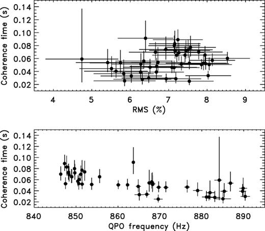
Top: QPO coherence time as a function of QPO rms for segment 1, when the QPO disappeared at about 890 Hz. Bottom: QPO coherence time versus QPO frequency for the same segment of data. To reduce scattering in the data points, the averaging time for the PDS is 64 s instead of 32 s.
We have investigated whether these trends were present in the whole data set, in which the frequency spans a much wider range. The relationship between the coherence time and  for all the data analysed here is shown in Fig. 5. To compute the coherence time, we have used
  from Table 1. There is a clear positive correlation between the two quantities until
  reaches a maximum level around ∼800 Hz (albeit with some scatter). After the maximum, an anticorrelation between the QPO frequency and coherence time, of the type seen within segment 1, seems to be present. A similar behaviour was reported from 4U 1636−53 for its lower kHz QPO (Di Salvo, Méndez & van der Klis 2003; see also van der Klis et al. 1997 for the upper kHz QPO of Sco X-1).
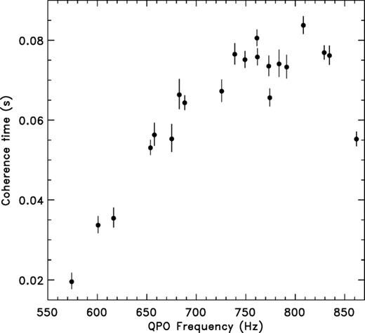
Dependence of the QPO coherence time on frequency.
The overall relationship between the rms amplitude of the QPO and its coherence time is shown in Fig. 6. The behaviour is much more complex; both positive and negative correlations are seen. Again, the pattern seen in segment 1 is not typical.

Dependence of the QPO coherence time on rms. The numbering refers to Table 1.
2.4 Coherence of the higher-frequency QPO
We have searched for the second QPO in the data using the shifted 32-s PDS used above. We detect an otherwise invisible higher-frequency QPO in five of the 21 segments used here. A weaker signal is detected in segments 1–3, 13–15, 16–18 and 20–21, which we group to obtain a meaningful fit. The results of fitting the higher-frequency QPOs are listed in Table 3. Given the relatively large width of the high-frequency QPO, the window for the fit is 200 Hz on each side of the QPO peak, excluding the region around the lower-frequency QPO. These QPOs have been previously reported in Méndez et al. (1998a,b, 1999). What is noticeable is that the higher-frequency QPO is much broader than the lower one, with Q less than ∼10. This is a well-known observational fact (van der Klis 2000). Interestingly, there is no apparent correlation between the coherence time of the higher-frequency QPOs and its frequency (of the type seen in Fig. 5 for the lower-frequency QPO), but we note that the frequencies do not span a wide range and that the error bars are relatively large.

The higher-frequency QPOs detected after applying the shift-andadd procedure to the 32-s PDS. νshift is the frequency to which the 32-s PDS were shifted. Δνlow is the width of the low-frequency QPO. νhigh, Δνhigh and rmshigh are respectively the frequency, the width and the rms of the high-frequency QPO. To obtain reliable fits, segments 1–3, 13–15, 16–18 and 20–21 were grouped together. The errors are again computed as χ2 = χ2min + 1.
3 Discussion
We have carried out a systematic study of the kHz QPO of 4U 1608−52, with the aim of investigating the coherence time of the underlying oscillator. By following the lower kHz QPO over the shortest time-scales permitted by the data statistics (down to 32 s) to minimize the contribution of the long-term frequency drifts, with a shift-and-add technique, we have found a lower limit on the quality factor larger than ∼150 in 14 of the 21 segments of analysed data. We have shown that in this object Q is as high as 200 for thousands of seconds. In many sources, the strength of the signal does not allow the study of the QPOs on such short time-scales, which may explain why the values of Q reported in the literature are generally lower than this.
Frequency drifts as large as 5 Hz are observed between consecutive 32-s PDS. In an attempt to remove the contribution of this short-term drift to the width of the QPO, we have applied the shift-and-add procedure to the 1-s PDS, using a sliding-window technique to estimate the QPO frequency every second. If the frequency drift were linear over 32 s, this method should remove the drift contribution to the width measured on 32 s and provide an estimate of the QPO width on a 1-s time-scale. Interestingly enough, the recovered QPO width is not significantly smaller than the width measured on 32 s. This surprising result could be explained by the fact that the error bars on the frequency are of the order of the expected gain, causing an artificial blurring of the QPO profile in the shift-and-add process. Alternatively, this might be an indication that the frequency, amplitude or phase of the underlying signal varies on time-scales much shorter than 32 s. In this case, this would most likely imply that the Q factor reported in Table 1 with the present technique underestimates the intrinsic Q of the QPO.
Determining the coherence time of the underlying oscillator from the width of the QPO over the wide range of frequency spanned (between 560 and 890 Hz), we have shown that there is a clear pattern in which the coherence time increases with frequency up to a maximum at ∼800 Hz. At both ends of the frequency range, the decreasing strength of the QPO seems to be associated with a decrease of both its amplitude and its coherence.
We now discuss the implications of the above results for QPO models. There are two different classes of models of the kHz QPOs: those involving clumps within or above the accretion disc (for a recent review see, for example, Miller, Lamb & Psaltis 1998; Stella & Vietri 1999; van der Klis 2004), and those involving oscillations of the disc (reviewed in Wagoner 1999 and Kato 2001).
3.1 Clumps
If inhomogeneities can form in the accretion flow in the form of clumps, which are more luminous than their surroundings and which orbit around the central star, the viewing geometry might be such that the clumps will produce luminosity variations (Bath 1973). Inhomogeneities lying at a radius R and having a radial extent ΔR will be sheared by differential rotation and will therefore have a finite lifetime. The maximum lifetime for such a clump to be stretched to an axisymmetric ring is given by τs= (2/3)(R/ΔR) Pk, where Pk is the Keplerian period at radius R (Bath, Evans & Papaloizou 1974). In the clump model, this lifetime is comparable to the coherence time of the QPO τ∼τs. Such clumps will produce a luminosity variation of at most ΔL/L=ΔR/R (Pringle 1981). Hence, τs∝R/ΔR∝ (ΔL/L)−1, so high coherence of the signal and its high amplitude are incompatible in the clump model. In our case ΔL/L is of the order of 10 per cent (see Fig. 6). This would imply τs∼ 10 Pk≲ 0.01 s (or Q∼ 30), much shorter than the coherence time we found in our analysis (see Fig. 5). It is also worth noting that in the above formula the clump lifetime (and signal amplitude) is predicted to decrease with increasing frequency (e.g. Livio & Bath 1982), unlike the observed behaviour in Figs 5 and 6.
This is clearly not what we observe in this source (see Fig. 6). Alternatively, one can make the assumption that the radial extent the blob is of the order of the disc height (h). Shakura & Sunyaev (1973) estimate h∼ 3 × 106 cm(L/LEdd) (M/M⊙), and that the radius of the relevant orbit is of the order of the stellar radius, or a few times larger. For an accreting neutron star with a large fraction of Eddington luminosity, h/R∼ 1/10 is a reasonable estimate, which again leads to the same conclusions.
We have also found that the higher-frequency kHz QPO is much fainter and is characterized by a much lower quality factor. This result is hard to reconcile with models in which the higher-frequency QPO is a Keplerian frequency at some radius (e.g. the sonic point; Miller et al. 1998), and the lower QPO is a beat frequency generated by interaction of the neutron star radiation with clumps originating at that particular radius. This model predicts that the width of the two QPOs should be similar, because the stellar spin frequency is expected to be highly coherent. In 4U 1608−52, we have shown the width of the higher-frequency QPO to be much larger than the width of the lower-frequency QPO.
Another model of QPOs has been proposed in which clumps leave the accretion disc and for some reason follow test particle orbits. In this so-called relativistic precession model (e.g. Stella & Vietri 1999), the clump is responsible for all three frequencies: two kHz QPOs and a lower-frequency QPO, also called the horizontal branch oscillation. Because the same agent is responsible for the two kHz QPOs, the coherence times should be about the same. We have shown here that the coherence time of the higher-frequency QPO is at least a factor of 10 lower than that of the lower-frequency QPO (see Table 3).
More stable non-linear structures (vortices) may persist in the accretion disc, but these will be subject to radial inflow unless they are anchored by an external magnetic field (Abramowicz et al. 1992; Lovelace et al. 1999; Tagger 2001). The inflow velocity at radius r in an α-disc of thickness h, is a factor of α(h/r)2 lower than the orbital velocity, where α > 10−2 is the dimensionless viscosity. So, for typical discs, within ∼10 orbits the fluid is carried inwards by a distance equal to a few per cent of its initial radius, and suffers a percentage change in orbital frequency which is 1.5 times larger.
Thus, all models of this class seem to be incompatible with a high Q factor, and the relationships found between the coherence time with frequency and rms amplitudes.
3.2 Disc oscillations
There is growing evidence that the oscillations originate in the disc itself, in particular because the same phenomena are observed in a wide range of accreting X-ray sources, from white dwarfs to black holes (Mauche 2002). Several models relating QPOs to disc oscillations have been proposed, some of them making clear predictions of what the quality factor of the QPO should be. This is the case, for instance, for the transition layer model proposed by Titarchuk, Lapidus & Muslimov (1998). In this model, a shock occurs where the Keplerian disc adjusts to the subKeplerian flow and the transition can undergo various types of oscillations under the influence of the gas, radiation, magnetic pressure and gravitational force. In this case, Q can in principle reach 100. It is expected to increase with frequency but also with luminosity (Titarchuk et al. 1998). In our data set it is clear that there is not a good correlation between Q and the source count rate.
For acoustic waves in isotropic turbulence, Goldreich & Kumar (1988) predict Q∼h/(λα). Here, α∼ 0.1 is the viscosity parameter for a Shakura–Sunyaev disc and the wavelength, λ, is much greater than h, yielding a rather low value of Q. Anisotropic turbulence increases this to Q=λ/(hα) ∼ 10, as observed in black holes. For g modes and isotropic turbulence, Q is the higher value of 1/α and  , but the highest values of Q are obtained for g modes in anisotropic turbulence, (r/h)/α∼ 100. For c modes, which correspond to a warp revolving at the Lense—Thirring frequency (a general relativistic effect), this value is enhanced by a factor approximately equal to the square of the ratio of orbital velocity to the speed of sound (the discussion in this section follows Ortega-Rodríguez & Wagoner 2000). In the very hot disc around the neutron stars, this enhancement may still be insufficient to explain the high Q reported here. However, some modes are excited, rather than damped, by viscosity and may enter the non-linear regime (Ortega-Rodríguez & Wagoner 2000).
4 Conclusions
We have shown that the kHz QPO in 4U 1608−52 is a highly coherent signal with an inferred coherence time of up to about one-tenth of a second. This result, as well as the dependence of the QPO coherence time on frequency and amplitude which we report, is hard to reconcile with QPO models involving orbiting clumps. This leaves the accretion disc oscillations as the most likely alternative for accounting for these signals.
Acknowledgments
We are grateful to Mariano Méndez, Michiel van der Klis and Bob Wagoner for very helpful discussions. WK acknowledges support by the Centre National de la Recherche Scientifique (CNRS) through a poste rouge, and thanks Centre d'Etude Spatiale des Rayonnements for hospitality. Research supported in part by LEA Astro-PF, and KBN through grant 2 P03D 014 24. SP acknowledges a grant from the Swiss National Science Foundation. We are grateful to an anonymous referee whose detailed and comprehensive comments helped to improve the clarity of the points made in this paper.
References
