Galaxy groups in the 2dFGRS: the group-finding algorithm and the 2PIGG catalogue Free

Abstract

1 Introduction

Groups of galaxies are useful tracers of large-scale structure. They provide sites in which to study the environmental dependence of galaxy properties, the galactic content of dark matter haloes, the small-scale clustering of galaxies, and the interaction between galaxies and hot X-ray emitting intragroup gas. Thus, it is desirable to have an extensive, homogeneous catalogue of groups of galaxies representing the various bound systems in the local universe.

Many studies in the past relied upon the pioneering work of Abell (1958) to provide a set of target galaxy clusters (see also Abell, Corwin & Olowin 1989; Lumsden et al. 1992; Dalton et al. 1997, for similar studies). However, because of the lack of redshift information available when Abell was defining his cluster catalogue, concerns have been raised over the completeness of his sample and the impact that line-of-sight projections would have in contaminating it (e.g. Lucey 1983; Sutherland 1988; Frenk et al. 1990; van Haarlem et al. 1997). As a result of these worries, it became fashionable to select galaxy cluster samples based upon cluster X-ray emission (e.g. Gioia et al. 1990; Romer 1995; Ebeling et al. 1996; Böhringer et al. 2001), this method being less prone to projection effects. This strategy nevertheless brings its own complications, because X-ray emission depends sensitively on the details of intracluster gas physics.

The construction of galaxy redshift surveys over the past 20 years has enabled a number of groups to pursue the optical route to group-finding. Huchra & Geller (1982), Geller & Huchra (1983), Nolthenius & White (1987), Ramella, Geller & Huchra (1989) and Moore, Frenk & White (1993) used subsets of the Centre for Astrophysics (CfA) redshift survey, containing a few thousand galaxies, to investigate both the abundance and the internal properties of samples of a few hundred galaxy groups. Maia, da Costa & Latham (1989) extended the data base using the Southern Sky Redshift Survey of a further ∼1500 galaxies and identified a sample of 87 groups containing at least two members. All-sky galaxy samples of ∼2400, 4000 and 6000 galaxies were used for group-finding by Tully (1987), Gourgoulhon, Chamaraux & Fouqué (1992) and Garcia (1993), respectively. Deeper surveys of small patches of sky have also been used to find groups by Ramella et al. (1999, ∼3000 galaxies) and Tucker et al. (2000, ∼24 000 galaxies). Giuricin et al. (2000), Merchán, Maia & Lambas (2000) and Ramella et al. (2002) have performed analyses on catalogues containing up to ∼20 000 galaxies, but the largest set of galaxy groups so far is that provided by Merchán & Zandivarez (2002). They used the ∼60 000 galaxies in the contiguous Northern and Southern Galactic Patches (NGP and SGP) in the ‘100k’ public data release of the Two-degree Field Galaxy Redshift Survey (2dFGRS; Colless et al. 2001). This work extends that sample to the NGP and SGP regions in the complete 2dFGRS.¹ The entire survey contains about 220 000 galaxies, ∼190 000 of which are in the two contiguous patches once the completeness cuts detailed below have been applied.

As well as using more galaxies than were previously available, this study also contains the results from rigorous tests of the group-finding algorithm. These are facilitated by the construction of very detailed mock 2dFGRSs, created using a combination of dark matter simulations and semi-analytical galaxy formation models. Comparing the properties of the recovered galaxy groups to those of the underlying parent dark matter haloes provides a robust framework within which the parameters of the group-finding algorithm can be chosen so as to apportion the galaxies optimally. Furthermore, the ability to relate, in a quantitative fashion, the input mass and galaxy distributions to the set of recovered galaxy groups, is of crucial importance when trying to extract scientific information from the group catalogue. This approach is identical in spirit to that adopted by Diaferio et al. (1999) when they studied the northern region of the CfA redshift survey.

The choice of group-finding algorithm is described in Section 2. Details of the mock catalogue construction and group-finder testing are given in Sections 3 and 4. Section 5 contains the results when the group-finder is applied to the real 2dFGRS.

2 The Group Finder

2.1 Choice of algorithm

Given a set of galaxies with angular positions on the sky and redshifts, the task of the group-finder is broadly to return sets of galaxies that are most likely to represent the true bound structures that are being traced by the observed galaxies. For some applications, not missing any of the true group members will be particularly desirable. For others, minimizing the amount of contamination by nearby, yet physically separate, objects will be the priority. It is inevitable that some distinct collapsed objects, situated near to each other in real space and along a similar line of sight, will be spread out by line-of-sight velocities to the extent that they overlap with one another. Thus, some unavoidable contamination is to be expected. The aim of the group-finder described here is to find a compromise between the extremes of finding all true members and minimizing contamination, with a view to providing groups that have velocity dispersions and projected sizes similar to those of their parent dark matter haloes. Naturally, the efficiency of such a group-finder can only be calibrated and tested when the properties of the associated dark matter haloes are known. The use of realistic mock catalogues is thus central to the entire group-finding procedure because it directly affects the composition of the final group catalogue through the choice of parameters for the group-finder.

To date, the job of finding groups in galaxy redshift surveys has typically been assigned to a percolation algorithm – see Tully (1987), Marinoni et al. (2002) and references within Trasarti-Battistoni (1998) for alternative approaches – that links together all galaxies within a particular linking volume centred on each galaxy. These friends-of-friends (FOF) algorithms are specified by the shape and size of the linking volume and how it varies throughout the survey. In order to produce galaxy groups corresponding to a similar overdensity throughout the survey, the linking volume should be scaled to take into account the varying number density of galaxies that are detected as a function of redshift. Previous studies have not all chosen the same scaling for the linking length with mean observed galaxy number density, n. At higher redshifts, flux-limited catalogues contain a lower number density of galaxies, causing the mean intergalaxy separation to increase. The algorithm proposed by Huchra & Geller (1982) scales both the perpendicular (in the plane of the sky) and the parallel (line-of-sight) linking lengths (ℓ_⊥ and ℓ_∼∼) in proportion to n^−1/3. Ramella et al. (1989) scaled both linking lengths in proportion to n^−1/2. In contrast, Nolthenius & White (1987) and Moore et al. (1993) chose to set ℓ_∼∼ to correspond to the typical size in redshift space of groups detected as a function of redshift. The perpendicular linking lengths were scaled in proportion to n^−1/2, this being how the mean projected separation varies. Thus, in contrast with the other methods, the aspect ratio of this linking volume is not independent of redshift.

In choosing how to scale the linking lengths, there is one primary condition that one would like to satisfy. Namely, that for a particular group of galaxies sampled at varying completeness, the edges of the recovered group should be in similar places. If this is achieved, then the inferred velocity dispersion and projected size and the actual contamination should be independent of the sampling rate. Scaling both ℓ_⊥ and ℓ_∼∼ by n^−1/3 will lead to groups of similar shape and overdensity being found throughout the survey. Of course, if the galaxy distribution is sampled very sparsely then this scaling can lead to linking lengths that are large with respect to the size of real gravitationally bound structures. So, depending upon the nature of the galaxy survey, it may be desirable to put an upper limit on the size of the linking volume. The maximum value of the perpendicular linking length is one of the parameters of the algorithm used here.

2.2 The linking volume

Having defined how the linking volume scales with mean observed galaxy number density, the choice of its shape and size still remains. The shape of the linking volume should clearly be spherical in the case where real galaxy distances are measured. However, with redshift space distances, groups will appear elongated along the line of sight, and one can appreciate that in order to find all of the group members, ℓ_∼∼ > ℓ_⊥ would be helpful. An approximate estimate of the amplitude of this stretching can be made by considering how rapidly galaxies will be moving in a halo of mass M and radius r. If the circular velocity satisfies v²=GM/r, the line-of-sight velocity dispersion can be written as σ²≈v²/2 and the total mass is M= 4/3πr³Δ_cρ_c, where ρ_c is the critical density and Δ_c defines the mean density relative to critical within the halo. Then

(2.1)

Setting Δ_c= 150 yields

(2.2)

(Note that, according to the spherical ‘top-hat’ model Δ_c≈ 100, 180 for Ω₀= 0.3, Λ₀= 0.7 and Ω₀= 1 models, respectively; Eke, Cole & Frenk 1996.) Thus, for an object with virial radius r, the velocities produce a 1σ stretch along the line of sight of ∼6r. The ratio of parallel to perpendicular sizes is independent of r. This ignores the redshift measurement errors which will add in an r-independent parallel contribution of σ_err∼ 85 km s⁻¹ for the 2dFGRS (Colless et al. 2001) with no corresponding perpendicular increase. Even at the lowest redshifts, this error term is smaller than the typical line-of-sight linking length for the 2dFGRS. Consequently, the shape of the linking volume should be elongated, with a particular aspect ratio given by R_gal=ℓ_∼∼/ℓ_⊥, and the appropriate value for this ratio should be ∼12 to enclose 2σ of the galaxies along the line of sight.

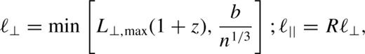
In dark matter N-body simulations, FOF group-finders are often applied in real space with a linking length that is b= 0.2 times the mean interparticle separation in order to identify groups having overdensities that are ∼b⁻³ (Davis et al. 1985). This choice of linking length has been shown by Jenkins et al. (2001) to yield a halo mass function that is independent of redshift and Ω₀, and thus provides a good definition of the underlying dark matter haloes. Because redshift space, rather than real space distance, is available in the 2dFGRS, it is unclear quite what value of b_gal, in terms of the mean intergalaxy separation, is appropriate to reproduce the boundary of the groups as defined by a b= 0.2 set of dark matter groups. The parameter b will be used to set the overall size of the linking volume through ℓ_⊥=b/n^1/3. The semi-analytical model of Cole et al. (2000) predicts that light is typically more concentrated than mass in groups. Thus, a value of b_gal smaller than 0.2 is likely to be appropriate for recovering the b= 0.2 set of dark matter groups from a galaxy survey.

This discussion implies that the linking volume should be elongated along the redshift direction, and provides rough expectations for both the aspect ratio and overall size of the volume that will best recover the underlying dark matter haloes. However, the precise shape of this volume is yet to be specified. Both a cylinder and an ellipsoid could satisfy the above requirements. In the absence of peculiar velocities, an ellipsoid reduces smoothly to the usual real space spherical linking volume, but tests on mock 2dFGRSs reveal that a cylinder is slightly more effective at recovering groups that trace the underlying dark matter haloes. This empirical motivation leads to a cylindrical linking volume being employed throughout this paper.

2.3 Empirically motivated fine tuning

While the picture painted in Section 2.2 is pleasingly simple, with both the aspect ratio and the linking volume being independent of group mass, in practice the optimum linking volume to recover the b= 0.2 set of dark matter groups from the galaxy survey is not quite this universal. There are a number of reasons why this similarity breaks down. For instance, the mass-to-light ratio in the mock catalogues varies with halo mass such that light is less concentrated in more massive clusters. Also, halo concentration depends on mass, and concentration affects the halo velocity structure and total enclosed overdensity (when the halo edge is defined by an isodensity contour). Using the galaxy population which sparsely samples the dark matter groups, these factors combine to yield a small systematic bias in the recovered group properties. Tests with mock catalogues have shown that this produces either small haloes with overestimated sizes (and velocity dispersions), or large clusters with sizes that are underestimated. Across the range of masses from 10¹³–10¹⁵h⁻¹ M_⊙ this amounts to a 20 per cent effect in the projected size and slightly smaller in the velocity dispersion. To correct for this requires knowledge of the halo mass in which each galaxy resides. An estimate of this quantity is made by measuring the galaxy density relative to the background in a cylinder with aspect ratio R_gal and a comoving projected size of 1.5 h⁻¹ Mpc. This density contrast, Δ, is then used to scale both the size and aspect ratio of the linking cylinder according to

(2.3)

and

(2.4)

where Δ_fit, ε_b and ε_R are parameters to be fitted from the mock catalogues. This enables the removal of the biases described above, while effectively increasing the spread in linking lengths at a given redshift by a few tens of per cent.

2.4 The mean galaxy number density

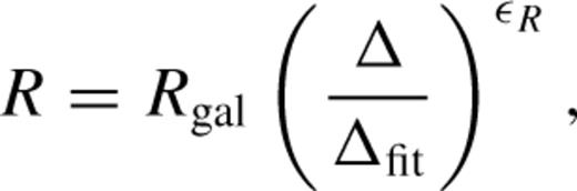
In addition to varying with redshift, the mean observed galaxy number density, n, depends on the depth to which a particular region of sky was surveyed, and the efficiency with which redshifts were measured. The production of maps that describe the angular variation of the survey magnitude limit, b^lim_J(θ), the redshift completeness, R(θ), and a function, μ(θ), related to the apparent magnitude dependence of the redshift completeness, is described in section 8 of Colless et al. (2001). These quantities, along with a galaxy weight, w, that models the local completeness of the 2dFGRS, were combined to define n at the position of each galaxy.

Galaxy weights were calculated by removing all fields in the 2dFGRS that have a completeness less than 70 per cent and then all sectors (areas defined by the overlap of 2dFGRS fields) that have a completeness less than 50 per cent. Rejecting all galaxies from fields of low completeness eliminates from the sample the small amount of data that were taken in poor observing conditions. Rejecting sectors with low completeness removes regions which are incomplete due to the fact that some 2dFGRS fields were not observed or are excluded by the above cut. Unit weight is then assigned to all the galaxies of the parent Automatic Plate Measuring (APM) catalogue in the remaining sectors. All of these galaxies without measured redshifts have their weight redistributed equally to their 10 nearest neighbours with measured redshifts. Because low completeness sectors are excluded, the weights produced are never large. Their mean value is 1.2 with an rms dispersion of 0.2. The inverse of the weight, 1/w, is a local measure of the completeness in the 2dFGRS around each galaxy.

The model for the redshift completeness as a function of apparent magnitude is

(2.5)

where γ is a normalization factor determined by the overall completeness in a given direction. The incompleteness in a given direction is a result not only of the failure to obtain redshifts for some of the faintest galaxies, but also of the failure to target galaxies either because the corresponding 2dFGRS field was not observed or because of constraints on the fibre positioning. To determine the completeness assumed in constructing the mock 2dFGRS catalogues, γ is set in each sector by demanding that the completeness averaged over apparent magnitude

(2.6)

be equal to the measured overall completeness, R(θ), in that sector. Here, the integrals are over the apparent magnitude range of the survey, from a global bright magnitude limit to the local faint magnitude limit. A simple power-law fit to the observed number counts, N(b_J) ∝ 10, is used. In contrast, to model the completeness in the genuine or constructed mock catalogue, γ is fixed at the position of each galaxy by demanding that . That is, the inverse of the weight assigned to each galaxy is taken as a local measure of the completeness in that direction. In the case of the genuine survey this has the advantage that it will automatically take account of any small-scale variation in the completeness that might occur due to the constraints on fibre positioning. Having fixed γ, the comoving number density of galaxies at each angular position and redshift is computed from the 2dFGRS luminosity function as

(2.7)

The luminosity function used here is that estimated by Norberg et al. (2002), convolved with their model of the 2dFGRS magnitude measurement errors.

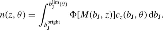
2.5 The linking criteria

Taking all of these survey characteristics into account, and defining a maximum perpendicular linking length in physical coordinates as L_⊥,max, the comoving linking lengths associated with a particular galaxy are

(2.8)

and two galaxies i and j, at comoving distances d_c,i and d_c,j with an angular separation θ_ij, are linked together if

(2.9)

and

(2.10)

The conversion of observed redshift to comoving distance (R₀χ) requires an assumption about the cosmological model. This impacts both on the inferred galaxy comoving space density, as n∝ (dV/ dz)⁻¹∝[R₀S(χ)]^2/3/H(z)^1/3 (see, for example, Peacock 1999) and on the comoving distance for a given redshift. The angle subtended by the chosen linking length-scales like θ∝n^−1/3/(R₀χ). Throughout this paper Ω₀= 0.3 and Λ₀= 0.7 will be used. This is appropriate for the mock catalogues and not obviously very wrong for the real one (Spergel et al. 2003). At the median survey redshift of 0.11, this model yields an angular linking length that is almost 2 per cent larger (and a comoving distance that is about 5 per cent larger) than an Einstein–de Sitter model.

3 Constructing A Mock 2dFGRS

It is clearly important to understand how the galaxy groups discovered by this percolation algorithm are related to the underlying distribution of dark matter in the Universe. To address this issue and, at the same time, determine the optimum set of parameters to use in the group-finder, mock 2dFGRSs have been constructed using high-resolution N-body simulations of cosmological volumes and a semi-analytical model of galaxy formation.

The main N-body simulation used is the Λ cold dark matter (CDM) GIF volume described by Jenkins et al. (1998). The density parameter is Ω₀= 0.3, the cosmological constant is Λ₀= 0.7 and the normalization of density fluctuations is set so that the present-day linear theory rms amplitude of mass fluctuations in spheres of radius 8 h⁻¹ Mpc, σ₈= 0.9. The box size is 141.3 h⁻¹ Mpc. Another simulation with 288³ particles in a ΛCDM box of length 154 h⁻¹ Mpc with σ₈= 0.71 has also been used to test the sensitivity of the optimum group-finding parameters to the amplitude of the mass fluctuations. It turns out that the optimum parameter choice is insensitive to this change in σ₈, although the amount of spurious contamination does increase by ∼10 per cent when this decrease in the contrast between groups and not groups is applied. The GIF volume will be used in the subsequent analysis.

Dark matter haloes are identified in these simulation cubes using a FOF algorithm with a linking length of b= 0.2 times the mean interparticle simulation. The kinetic and potential energies of grouped particles are computed and unbound particles are removed from the group. Bound groups of 10 or more particles are retained, giving a halo mass resolution of 1.4 × 10¹¹h⁻¹ M_⊙ (see Benson et al. 2001 for further details).

The reference semi-analytical galaxy formation model of Cole et al. (2000) is used to populate the bound haloes identified in the z= 0 output of the N-body simulation following the prescription outlined in Benson et al. (2000). The halo mass resolution of the N-body simulation in turn imposes a resolution limit in the semi-analytical calculation. This corresponds to the absolute magnitude of central galaxies that occupy dark matter haloes that have 10 or more particles. Scatter in the formation histories of galaxies and variable amounts of dust extinction cause a spread in the relationship between the luminosity of a central galaxy and the mass of the host halo. As a working definition, the magnitude limit of a z= 0 volume-limited galaxy catalogue constructed from the N-body simulation is taken to be M−5 log₁₀h=−17.5; at this luminosity, 90 per cent of central galaxies predicted in a semi-analytical model calculation without any halo mass limitations reside in haloes resolved by the simulation.

The luminosity resolution of the volume-limited catalogue, when combined with the global k+e correction adopted by Norberg et al. (2002), implies that a mock 2dFGRS survey constructed from this simulation output will only be complete above a redshift of z= 0.08. The median redshift of the 2dFGRS is z= 0.11, so it is desirable to extend the mock catalogue to fainter luminosities. This was done by constructing a volume-limited sample of galaxies from a separate semi-analytical calculation for haloes with masses less than the N-body resolution limit. These galaxies were then assigned at random to the particles in the simulation that were not part of a bound halo. This should be a reasonable approximation because the clustering of dark matter haloes is almost independent of mass for masses beneath the resolution limit of the GIF simulation (Jing 1998). Using this technique, the luminosity limit was shifted to M−5 log₁₀h=−16.0, so that a flux-limited catalogue constructed from this output would be complete above a redshift of z= 0.04.

A mock 2dFGRS was constructed from the volume-limited galaxy catalogue by applying the following steps.

• (i)

  A monotonic transformation was applied to the magnitudes given by the semi-analytical model, perturbing them slightly so as to reproduce the 2dFGRS luminosity function. The reason for doing this is that the galaxy luminosity function of the semi-analytical model is not a perfect match to the measured 2dFGRS luminosity function (Benson et al. 2000) and it is desirable that the selection function of the mock catalogue should accurately match that of the genuine survey. The magnitudes are then perturbed using the model of the 2dFGRS magnitude measurement errors described in Norberg et al. (2002).

• (ii)

  The volume-limited catalogue was replicated, about a randomly located observer, to take into account the much greater depth of the 2dFGRS volume compared to the size of the N-body simulation box. This has no impact upon the tests of the group-finder presented here, although it does mean that the mock catalogue is unsuitable for studying the clustering of groups on scales approaching the size of the simulation box.

• (iii)

  Galaxies were then selected from within this volume by applying the geometric and apparent magnitude limits of the 2dFGRS survey defined by the map, b^lim_J(θ), of the survey magnitude limit (see Section 2 and Colless et al. 2001, section 8). This produces a mock catalogue in which every galaxy has a redshift.

• (iv)

  The appropriate redshift completeness was then imposed sector by sector on the mock catalogue, by randomly retaining galaxies so as to satisfy the function c_z(b_J, θ) (equation 2.5).

This method ignores any systematic variation of the completeness within a sector, and in particular it does not take account of close-pair incompleteness on angular scales less than ∼0.75 arcmin. To investigate the effect of this, a second set of mocks was also produced, in which close pairs were identified in the parent mock catalogue and preferentially rejected when reproducing the incompleteness in each sector. Not all close pairs are missed in the 2dFGRS because the large overlaps between 2dFGRS fields permits different members of close pairs to be targeted on different fields. One statistic that can be used to quantify the level of close-pair incompleteness is the ratio of the angular correlation function of objects that have measured redshifts to that of the full parent catalogue (Hawkins et al. 2003). To reproduce the appropriate level of close-pair incompleteness in the mock catalogue, the parameters of the rejection algorithm (the angular scale of the close pairs and the fraction that are rejected) were tuned so as to reproduce this statistic. In practice, the recovered groups hardly varied at all with the inclusion of the close-pair incompleteness. This is because of the combination of the large amount of field overlap in the 2dFGRS and the small angles over which fibre clashes become important.

Every galaxy in the mock survey is either spawned by a dark matter halo containing at least 10 particles or is a background galaxy that is located at the position of an ungrouped dark matter particle. In the following section, the phrase ‘the number of galaxies spawned by a particular dark matter halo’ will be used to refer to the subset of galaxies belonging to that halo which make it through the observing procedure and into the mock survey.

The use of a realistic mock 2dFGRS catalogue to set the parameters required for the group-finder and to interpret the nature of the derived groups represents a clear advance over previous work, which either neglected to present any such tests or, at best, used mock catalogues constructed from dark matter only simulations. One criticism that could be levelled at the approach presented here is that it is model-dependent. However, direct tests have been performed to confirm that the optimum group-finding parameters are insensitive to catalogues created with a 20 per cent lower value of σ₈ (and appropriate adjustments to the semi-analytical galaxy formation model). It should be borne in mind that the default model does provide a very reasonable description of the real Universe. In particular, it is in excellent agreement with a number of observables that have a direct bearing on group-finding in the 2dFGRS: the local luminosity function in the b_J-band (see fig. 10 of Madgwick et al. 2002; Cole et al. 2000), the clustering of luminous galaxies (Benson et al. 2000) and the dependence of galaxy clustering on luminosity (Benson et al. 2001; Norberg et al. 2001). Any alternative model would also need to reproduce all of these relevant observations for the testing of the group-finder to be similarly appropriate.

4 Testing the Group-Finder

4.1 Definitions

The mock surveys, complete with their parent dark matter haloes, provide a data base on which to optimize the parameters of the group-finder. These are mainly the maximum perpendicular linking length (L_⊥,max), the aspect ratio of the linking cylinder (R_gal) and the number of mean intergalaxy separations defining the perpendicular linking length (b_gal). In the remainder of this paper, the additional tweaks to the linking volume described in Section 2 will be set to values obtained empirically:

(4.1)

The process of deciding which is the best set of group-finding parameters requires a definition of what is good. A good group-finder should find a high fraction of the available groups, provide accurate estimates of their size and velocity dispersion, avoid splitting them up into subgroups and minimize the number of interloping galaxies. In an attempt to quantify these qualities, the following four statistics have been defined.

• (i)

  Completeness, c, is the fraction of detectable dark matter haloes that have more than half of their spawned galaxies in a single galaxy group. A dark matter halo is detectable if it spawns at least two galaxies into the mock survey.

• (ii)

  The median accuracy, a_σ or a_r, is the median log₁₀ of the ratio of associated galaxy group to dark matter group velocity dispersion or projected size. The associated galaxy group is the one that both contains the largest number of the galaxies spawned by this dark matter halo (or the group with most members overall if there is a tie), and is associated to this halo. A galaxy group is associated with the dark matter halo that spawned most of its members. If this is not unique, then the most massive of the possible dark matter haloes is chosen. With these definitions, it is possible for more than one galaxy group to be associated with the same dark matter halo, but that dark matter halo will have only one associated galaxy group. The set of values from which a_σ and a_r come is constructed by matching every detected dark matter halo with its associated galaxy group. A detected dark matter halo is one with an associated galaxy group. The spread about the median is described by the semi-interquartile range, s_σ or s_r.

• (iii)

  Fragmentation, ƒ, is the mean number of extra galaxy groups per dark matter halo having mass, defined later in this subsection, at least 0.2 times that of their associated dark matter halo for all detected dark matter haloes.

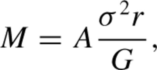
• (iv)
  The quality, q, of an individual halo to group match is defined as

  

  (4.2)

  where N_good is the number of member galaxies spawned by this halo that are found in the associated galaxy group, N_bad is the number of group members not spawned by this halo and N_spawn is the total number of galaxies spawned by this dark matter halo.

The velocity dispersions of the galaxy groups were calculated using a variant of the gapper estimator described by Beers et al. (1990). This is an efficient estimator that is resistant to outlying velocities. Tests on groups found from mock catalogues showed that this estimator gave an a_σ that varied less with the minimum number of galaxies per group than other choices. The gapper estimator also yielded an s_σ that was at least as low as the others for groups of all sizes. In detail, this involves ordering the set of recession velocities {v_i} of the N group members and defining gaps as

(4.3)

Using the following weights

(4.4)

the gapper estimate of the velocity dispersion can then be written as

(4.5)

Under the assumption that one of the galaxies is moving at the centre-of-mass velocity of the halo, which is certainly true for the mock catalogues, the estimated velocity dispersion is multiplied by an extra factor of before the redshift measurement error, σ_err, is removed in quadrature, giving

(4.6)

Velocity dispersions of the parent haloes, which inevitably have many more dark matter particles in them than there are galaxies in the associated groups, were calculated as the rms velocity difference from the mean.

The projected size of groups and haloes, r, is defined as the weighted rms projected separation from the group centre of the members. This calculation is performed taking into account the galaxy weights resulting from the variable incompleteness, as described in Section 2.4. The centre is defined using an iterative method that first calculates the arithmetic weighted mean position of the remaining galaxies then rejects the most distant galaxy. When only two galaxies remain, the position of the galaxy with a larger weight, or if these are the same, the larger flux, is deemed to represent the group centre. The projected group size is then the weighted rms projected physical separation of the other N− 1 galaxies from this central galaxy. This measurement, in conjunction with the velocity dispersion, can be used to estimate the group mass as

(4.7)

where the value of A was chosen so that, for the optimum choice of group-finding parameters described later in this section, the median mass was unbiased. This led to a choice of A= 5.0. The fragmentation statistic was calculated using these galaxy group masses.

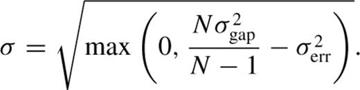
These definitions provide a framework within which comparisons can be made between group catalogues returned by different group-finding parameters. A good set of parameter values will yield a set of galaxy groups that have a completeness near to 1, a median accuracy of 0 (this being the log of the ratio of measured to true velocity dispersion or radius), independent of the group mass or redshift, with a small spread about this median, a fragmentation near to 0, and a quality of ∼1.

4.2 Parameter optimization

In Section 2, the three main free parameters of the group-finder were described. These determine the overall size of the linking volume through b_gal, the maximum size of the linking volume via L_⊥,max and the aspect ratio of the linking volume, defined by R_gal. Applying the group-finder to the mock catalogues described in Section 3 using various group-finding parameters, the recovered galaxy groups can be compared with their parent dark matter haloes, and the optimum set of parameters can be found. The following three subsections detail the effect of varying each of these parameters individually.

4.2.1 Varying L_⊥,max

The appropriate value for the maximum perpendicular linking length, L_⊥,max, should be similar to the size of the typical objects that are detectable at larger redshifts, where the number density of galaxies is low and this limit becomes relevant. Values around a couple of physical h⁻¹ Mpc are therefore a good place to search. R_gal= 11 and b_gal= 0.13 have been fixed. The justification for choosing these particular parameter values is contained in the following two subsections. Fig. 1 shows the behaviour of the comoving perpendicular linking length with redshift for L_⊥,max= 2 h⁻¹ Mpc. The increase of ℓ_⊥ with redshift reflects the decreasing mean observed number density of galaxies, and the spread in linking length at a given redshift comes from the angular variation in survey depth and the fraction of galaxies with measured redshifts. Larger values of L_⊥,max lead to larger linking volumes at the highest redshifts and some associated additional contamination. Decreasing L_⊥,max yields underestimates of the projected sizes and velocity dispersions of the groups at redshifts where the limit affects the size of the linking volume. Thus, L_⊥,max= 2 h⁻¹ Mpc is chosen as a physically motivated compromise.

Figure 1.

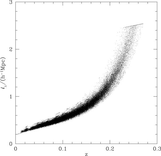
The variation of the comoving perpendicular linking length with redshift when L_⊥,max= 2 h⁻¹ Mpc and b_gal= 0.13 for each galaxy in a mock SGP. Note that the parameter L_⊥,max is in physical coordinates, whereas ℓ_⊥ is in comoving coordinates.

Open in new tabDownload slide

4.2.2 Varying R_gal

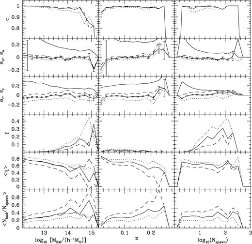
As was estimated in Section 2, the appropriate choice for the axial ratio of the linking cylinder is ∼10. A variety of values surrounding this one have been tried in conjunction with L_⊥,max= 2 h⁻¹ Mpc and b_gal= 0.13. Fig. 2 compares the properties of the dark matter haloes with those of their associated galaxy groups. The projected group sizes are fairly insensitive to R_gal as would be expected considering that these changes only impact upon the line-of-sight linking length. In contrast, the velocity dispersions are affected, and the more elongated linking volumes yield larger values, with an unbiased median being returned when R_gal≈ 11. As the linking volume is stretched, the completeness, fragmentation and quality change only very slightly, with the most significant change being a decrease of the quality of the group matches at higher redshift. Note that the drop in quality for the most massive haloes is driven by the large number of high-redshift, poorly sampled groups. To illustrate this, an additional long-dashed line is included in the lowest two panels in the first column of Fig. 2 showing the results using only the groups at z < 0.15. This demonstrates that considering only the nearby, well-sampled massive groups yields a mean halo quality, and interloper content, that is comparable with the lower mass haloes. Using the requirement that the median velocity dispersion be faithfully measured selects R_gal= 11 as the best choice. This is comparable with that suggested by the rough calculation leading to equation (2.2). Note that, without the additional halo mass dependent tweaks to the linking volume discussed in Section 2, the values of which are given in Section 4.1, there would be a gradient of ∼− 0.05 in all median accuracy curves as a function of dark matter halo mass.

Figure 2.

The effect of varying R_gal for an SGP mock catalogue. L_⊥,max and b_gal are held fixed at 2 h⁻¹ Mpc and 0.13, respectively, and R_gal is given values of 7 (dotted), 11 (solid) and 15 (dashed). The top row shows the mean completeness as a function of dark halo mass, redshift and number of galaxies spawned by the dark matter halo. The next rows show the median accuracies of the velocity dispersions and projected sizes of the galaxy groups, and the spread around the median value for the R_gal= 11 case (upper solid lines without error bars). The 1σ errors shown on the median R_gal= 11 curves are the errors on the mean accuracy calculated from the spread, assuming that the individual accuracies are distributed in a Gaussian fashion. The mean number of additional galaxy groups associated with detected dark matter haloes, as parametrized by the fragmentation, is displayed in the next row, followed by the mean quality of the group to halo matches in the penultimate row. This provides information about the difference between the numbers of good and bad member galaxies. The mean number of bad interlopers relative to the number of galaxies spawned by the parent halo is shown in the final row. An extra long-dashed curve is shown in the two lowest panels in the first column to show how the quality of high mass halo matches improves when only z < 0.15 groups are considered for the case of R_gal= 11. This also produces a corresponding decrease in the fraction of interlopers, as shown in the bottom panel.

Open in new tabDownload slide

4.2.3 Varying b_gal

Keeping L_⊥,max= 2 h⁻¹ Mpc and R_gal= 11 fixed, the value of b_gal, the number of mean intergalaxy separations defining the perpendicular linking length, was varied from 0.11 up to 0.15, and the parent b= 0.2 dark matter haloes were again compared with the resulting galaxy groups. Fig. 3 shows the results. As the linking lengths are increased, the recovered median group velocity dispersions and projected sizes also increase as larger volumes are grouped together. This is in contrast to the results when R_gal was varied and only the velocity dispersions were much affected. These changes are significant for all parent dark matter halo masses. Along with these variations, the increasing linking lengths increase completeness, reduce fragmentation and decrease the quality of the matches. The least biased accuracies are produced when b_gal= 0.13, and this is the value adopted for the rest of this paper.

Figure 3.

The effect of varying b_gal for an SGP mock catalogue. With L_⊥,max= 2 h⁻¹ Mpc and R_gal= 11, b_gal was given values of 0.11 (dotted), 0.13 (solid, and long-dashed for the z < 0.15 subset in the two lowest panels in the first column) and 0.15 (dashed). All quantities shown are the same as those in Fig. 2.

Open in new tabDownload slide

4.3 Summary of group-finding parameters

The results from the testing described in the previous three subsections suggest that an appropriate choice of group-finding parameters is L_⊥,max= 2 h⁻¹ Mpc, R_gal= 11 and b_gal= 0.13. These provide a set of groups that have unbiased velocity dispersions and sizes. In doing this, they contain almost all of the galaxies that should be included in groups with at least two members, and some interlopers as well. Smaller values of all of the above three parameters should be employed if reducing contamination is of greater importance than capturing as many true group members while not overestimating the velocity dispersion or projected size. The level of contamination in the groups found by this particular choice of group-finding parameters is illustrated in Fig. 4. This shows the redshift dependence of ratios of the memberships of the following three sets: (i) t, representing all galaxies in the mock survey, (ii) g, representing all grouped galaxies and (iii) l, representing galaxies that come from dark matter haloes which have spawned at least two galaxies into the mock survey, i.e. those that could be linked to another galaxy spawned by the same parent halo. gl is used to denote the overlap between sets g and l, and N_i is the membership of group i.

Figure 4.

The redshift dependence of ratios of the memberships of the three sets described in the text. The labels on the y-axis are ordered from bottom to top like the curves at z= 0.1. Thus, the fraction of all galaxies that have been spawned by haloes that spawn at least two galaxies (N_l/N_t) is shown with the solid line. The long-dashed curve shows the fraction of all galaxies that are put into groups (N_g/N_t). The short-dashed curve traces the fraction of grouped galaxies that are in set l. The dotted line shows the fraction of the N_l galaxies that are actually put into groups (N_gl/N_l), and the dot-dashed curve displays the ratio of the number of grouped galaxies to the number in set l.

Open in new tabDownload slide

The dotted curve in Fig. 4 shows that the detected groups contain almost all of the galaxies that belong in set l for all redshifts. For redshifts less than 0.1, the fraction of all galaxies that are grouped is ∼0.60, as shown by the long-dashed curve, whereas the solid curve shows that the fraction of all galaxies in set l is only ∼0.4. Of the grouped galaxies in this redshift range, only about 70 per cent of them are members of set l. This quantity is shown by the short-dashed line in Fig. 4.

The accuracy statistic relates only to the dark matter haloes that have spawned at least two galaxies (i.e. the detectable haloes), and have at least one associated galaxy group. For the above choice of group-finding parameters, about 51 per cent of galaxy groups are the best matches to detectable dark matter haloes, ∼47 per cent are associated with dark matter haloes that have only spawned one galaxy, ∼2 per cent are other matches with dark matter haloes and the remaining ∼0.2 per cent are made up completely from background galaxies that have been spawned by no well-defined dark matter halo. Thus, a significant fraction of the recovered groups are not being used to determine the group-finding parameters. These groups usually have velocity dispersions and projected sizes that are larger than those of their parent dark matter haloes. Consequently, the measured velocity dispersion and projected size for typical groups containing two galaxies, will be overestimates of those of the underlying dark matter halo. However, it would be inappropriate to adapt the group-finding parameters to be unbiased when these spurious groups are included, because this would inevitably spoil the results for the good matches.

5 Application to the 2dFGRS

Together, the NGP and SGP regions in the 2dFGRS contain 191 440 galaxies once cuts of 70 and 50 per cent have been applied for field and sector completeness, respectively. This set of galaxies, with their appropriate weights so that the mean observed galaxy number density n can be defined for each galaxy according to equation (2.7), has been used along with the FOF group-finder described in Section 2 with L_⊥,max= 2 h⁻¹ Mpc, R_gal= 11 and b_gal= 0.13, in order to find ‘real’ galaxy groups. The resulting catalogue places 55 per cent of all of the galaxies within 28 877 groups with at least two members. A total of 7020 groups are found with at least four members, and their median redshift and velocity dispersion are 0.11 and 260 km s⁻¹, respectively. The corresponding quantities for the sets of groups with at least three or five members are (N_groups, median z, median σ/km s⁻¹) = (12 566, 0.11, 227) and (4503, 0.11, 286).

The spatial distribution of the 2dFGRS Percolation-Inferred Galaxy Groups (2PIGGs) containing at least four galaxies is illustrated in Fig. 5. Each dot represents a group, with the colour and size representing the group velocity dispersion and unweighted galaxy content, respectively. Typical dot sizes decrease at large redshifts because the flux-limited survey means that large distant groups are sampled with only a few bright galaxies. At z≳ 0.15 the typical velocity dispersion also grows. This occurs both because only the bigger groups have enough bright galaxies to be recovered, and the smaller group memberships produce larger errors on the measured velocity dispersions, thus increasing the abundance of groups with apparently large velocity dispersions. Fig. 6 shows the distributions of these groups with respect to redshift, velocity dispersion, mass and weighted number of members, for the NGP and SGP strips of the survey. While the SGP has almost 50 per cent more galaxies in it than the NGP, the fraction grouped (0.56 and 0.54 for the NGP and SGP, respectively) and the distributions of properties of the resulting groups are very similar. The main difference is in the redshift distribution of groups, where the lower flux limit in the SGP betrays itself with a more extended distribution than the NGP. Consequently, a few extra high velocity dispersion, or equivalently high mass, clusters are found in the south. Although they are not reproduced here, these distributions of group properties are well matched to those found from the mock catalogues that were used to calibrate the group-finder.

Figure 5.

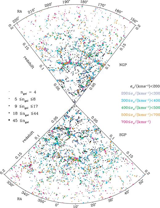
The spatial distribution of groups containing at least four members in the NGP and SGP regions. Dot colour and size represent the group velocity dispersion and unweighted number of members respectively, as shown in the legend.

Open in new tabDownload slide

Figure 6.

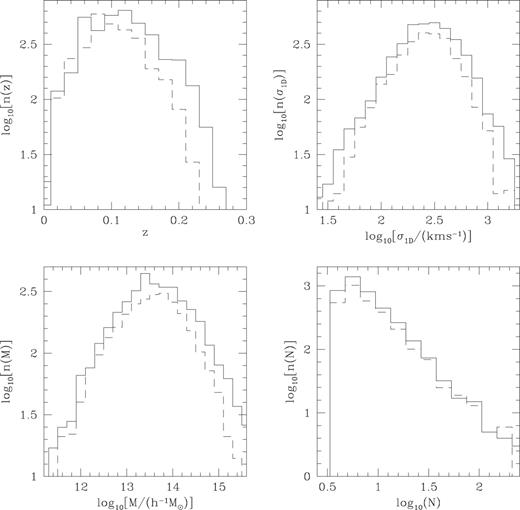
Histograms showing the distribution of group redshifts, velocity dispersions, masses and the weighted number of members from the real data. Only groups containing at least four members have been included. The solid and dashed histograms show groups found in the SGP and NGP, respectively.

Open in new tabDownload slide

Figs 7 and 8 show how the group memberships and velocity dispersions vary with redshift. This ties together the information contained in Figs 5 and 6, showing how the typical number of galaxies per group decreases with increasing redshift, while the velocity dispersion increases with increasing redshift.

Figure 7.

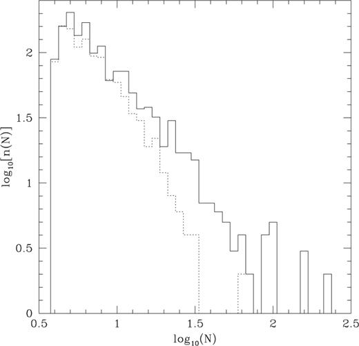
Histograms showing the distribution of weighted group memberships for groups containing at least four galaxies. These combine the data from NGP and SGP, and include groups in the following two redshift ranges: 0.04 ≤z≤ 0.08 (solid) and 0.14 ≤z≤ 0.18 (dotted).

Open in new tabDownload slide

Figure 8.

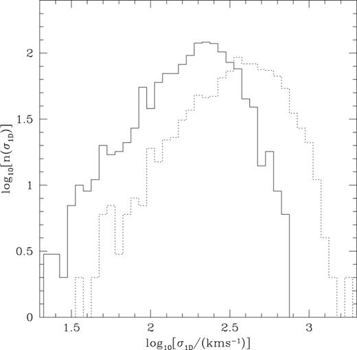
Histograms showing the distribution of velocity dispersions for groups containing at least four galaxies. These combine the data from NGP and SGP, and include groups in the following two redshift ranges: 0.04 ≤z≤ 0.08 (solid) and 0.14 ≤z≤ 0.18 (dotted).

Open in new tabDownload slide

One interesting comparison can be made with the results of Merchán & Zandivarez (2002). They used the public 100k data release version of the 2dFGRS and defined groups with a percolation algorithm similar to the one used here. For 2PIGGs containing at least four members, the mean redshift and velocity dispersion, 0.11 and 260 km s⁻¹, are very similar to their values of 0.105 and 261 km s⁻¹. The total number of these groups has increased from the 2209 that Merchán & Zandivarez found to 7020 in the 2PIGG catalogue. This factor is similar to the increase in the total numbers of galaxies being used, i.e. roughly the same fraction of galaxies are being grouped in both cases.

6 Conclusions

A FOF percolation algorithm has been described, calibrated and tested using mock 2dFGRSs and then applied to the real 2dFGRS in order to construct the 2PIGG catalogue.

From the mock catalogues, it is possible to determine the typical accuracies with which velocity dispersions and projected halo sizes are recovered. For detectable haloes recovered with galaxy groups containing at least four members, the estimates of the velocity dispersion are unbiased in the median and the ratio of inferred to true velocity dispersion has a semi-interquartile range of ∼30 per cent. The corresponding number for the spread about the median ratio of inferred to true projected size is ∼35 per cent. Without the use of detailed mock catalogues to calibrate the group-finder, the ability to derive science from the 2PIGG catalogue would be compromised by the uncertainty in how the recovered groups related to the underlying distribution of matter. This is thus a crucial step in the group-finding procedure.

When applied to the two contiguous patches in the real 2dFGRS, containing ∼190 000 galaxies, this percolation algorithm groups 55 per cent of the galaxies into ∼29 000 groups containing at least two members. Focusing on those groups with at least four members, their median redshift and velocity dispersion are 0.11 and 260 km s⁻¹, respectively. More detailed distributions of fundamental group properties are characterized in Section 5.

This 2PIGG catalogue is the largest currently available set of groups. It should provide a useful starting point for a number of studies concerning large-scale structure, galaxy group properties and the environmental dependence of galaxy properties. Upcoming papers will describe in more detail the contents of the groups, for instance the galaxy luminosity functions within groups, the mass-to-light ratios of groups, the manner in which galaxies are apportioned to different groups and the spatial distribution of galaxies within groups. The spatial abundance of groups, as a function of both total group luminosity and mass, will also be investigated. The catalogue, including basic group properties, is available on the World Wide Web, at http://www.mso.anu.edu.au/2dFGRS/Public/2PIGG/. A description of the contents of this web page is given in the appendix.

Acknowledgments

VRE and CMB are Royal Society University Research Fellows. JAP is grateful for a PPARC Senior Research Fellowship.

References

Appendix

Appendix A: Details of the Contents of the Web Page

The web page http://www.mso.anu.edu.au/2dFGRS/Public/2PIGG/ contains:

• (i)

  the lists (NGP and SGP) of galaxies and the index of the groups in which they are placed;

• (ii)

  lists of group properties for the 2PIGGs;

• (iii)

  the equivalent lists for some mock catalogues.

To illustrate the types of data that are available, Table A1 shows the information provided for a subset of the galaxies and Table A2 contains a list of all 2PIGGs containing at least 100 members.

Table A1.

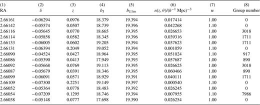
Data for a small subset of the galaxies in the NGP. The quantities listed for each galaxy are: (1) right ascension in radians (1950 coordinates); (2) declination in radians (1950 coordinates); (3) redshift; (4) b_J magnitude; (5) limiting b_J magnitude at this point in the survey; (6) n(z, γ) at this point in the survey (see equation 2.7); (7) galaxy weight, w, as described in Section 2.4; (8) the group number to which each galaxy is assigned (zero is ungrouped).

Open in new tabDownload slide

Table A2.

Data for all 2PIGGs containing at least 100 galaxies. The group quantities listed are: (1) number of member galaxies; (2) right ascension of the group centre in radians (1950 coordinates); (3) declination of the group centre in radians (1950 coordinates); (4) group redshift; (5) rms projected galaxy separation in h⁻¹ Mpc; (6) group velocity dispersion in km s⁻¹.

Open in new tabDownload slide