Collimation of a central wind by a disc-associated magnetic field Free

Abstract

1 Introduction

Several decades of observing young stellar objects (YSOs) have revealed a ubiquitous coincidence of structured outflows and accretion discs, accompanying the star-formation process. See Eislöffel et al. (2000), Königl & Pudritz (2000) and Reipurth & Bally (2001) for detailed reviews of Herbig–Haro (HH) objects and YSO outflows in general. The outflows are invariably collimated to some degree and always travel nearly perpendicular to accretion discs. Often, relatively wide-angle molecular (e.g. CO) outflows escort narrower optical outflows from the same source. The optical outflows typically consist of jets, which are often resolved into knots (HH objects), moving with bulk velocities of 100–200 km s⁻¹ and occasionally exhibit high degrees of collimation. The molecular outflows are slower, moving at a few tens of km s⁻¹. The question of whether CO outflows originate from physically distinct, wide-angle winds (e.g. Kwan & Tademaru 1988) or whether they result from momentum transferred to molecular cloud material from the jet (e.g. Königl & Pudritz 2000) has not been answered (Reipurth & Bally 2001; Lery et al. 2002).

Kwan & Tademaru (1988, 1995) review high spectral resolution observations of the central regions of young stellar systems at the origin of collimated outflows. They point out that several characteristics of optical forbidden emission lines are most easily explained by the presence of two winds of different origin. The two winds consist of the following:

• (i)

  a fast (≳100 km s⁻¹) wind originating from the very central region of the accretion disc or from the star itself; and

• (ii)

  a slow (∼10 km s⁻¹) wind launched from the outer (>10 R_⊙) region of the accretion disc (the ‘disc wind’).

Evidence for at least two, physically distinct winds exists for several objects (e.g. Solf & Böhm 1993; Fridlund & Liseau 1998; Bacciotti et al. 2000; Pyo et al. 2002).

Prevalent theoretical models for winds launched from accretion discs (see, e.g. Shibata & Kudoh 1999; Königl & Pudritz 2000, for a review) hold that the final wind velocity is of the order of the Keplerian rotational velocity of the launch point. The high velocity of observed optical jets suggests that they originate from a deep potential well (Kwan & Tademaru 1988), requiring the launching region to be much less than an astronomical unit (au) in extent, for reasonable parameters. To within observational limits, the jets often appear to emerge from their source with relatively large widths (several tens of au), but remain highly collimated immediately afterward (e.g. Burrows et al. 1996; Eislöffel et al. 2000; Reipurth et al. 2000, 2002). We therefore adopt the view that jets are launched from a region within several stellar radii, initially with large opening angles (hereafter the ‘central’ or ‘wide-angle’ wind), but then become collimated within several tens of au.

In wind-launching theory, the self-collimation of the wide-angle wind (due to azimuthal magnetic fields carried in the wind itself) cannot occur for all of the wind material (Blandford & Payne 1982; Sakurai 1985; Shu et al. 1995). In other words, without an external influence on the wind, the launching models predict that there is always some material leaving at very wide angles. On the other hand, theoretical studies of jets propagating into the surrounding environment most often assume that the flow is completely collimated (Frank, Gardiner & Lery 2002). Thus, there exists a gap in the theory between the launching and the propagation of YSO outflows. There is a need to understand how the initially wide-angle flows interact with their environment, presumably leading to a collimation of the entire flow.

Recent work by Gardiner, Frank & Hartmann (2003, also see references therein) considered the interaction of wide-angle winds with an unmagnetized, collapsing environment. They convincingly demonstrated that such flows may be collimated by shock focusing, especially when azimuthal magnetic fields are present in the wide-angle wind. For the central wind, they adopted a flow similar to that predicted by wind-launching theory on large scales, though they were unable to model the launching of the flow directly. As a result, all of the ambient material, even that in the equatorial plane, was swept away in the wind, preventing any further accretion into the central region. This is in contrast to the expectation from a system containing an accretion disc, which prevents any outflow in a direction near the equatorial plane. In this paper, we consider the interaction of a wide-angle wind with a magnetized environment. Our method allows us to follow the details of the launching of the wide-angle flow from a region very near the central star, while still following the wind out to tens of au, where it interacts with its environment.

Since the central, wide-angle winds become collimated along the rotational axis of the accretion disc, the collimation process itself must be associated with the angular momentum of the system. In this paper, we use numerical magnetohydrodynamic (MHD) simulations to explore the suggestion of Kwan & Tademaru (1988) that disc-associated magnetic fields collimate a central, fast wind into an optical jet. Large-scale disc fields may be generated by currents in the disc (Spruit, Foglizzo & Stehle 1997), or they could be embedded in the surface of the disc and carried outward in a slow disc wind (e.g. Blandford & Payne 1982; Pudritz & Norman 1983; Uchida & Shibata 1985; Pudritz & Norman 1986; Shibata & Uchida 1986; Kwan & Tademaru 1988; Shibata & Uchida 1990; Ouyed & Pudritz 1997; Ustyugova et al. 1999). We adopt an initially vertical field to approximate the magnetic configuration expected from a disc on scales that are large compared to the wind-launching region, but small compared to the size of the disc (e.g. Blandford & Payne 1982; Spruit et al. 1997). The disc fields we consider are very weak compared to those that are likely to be involved in launching the central outflow (e.g. fields near the surface of the star). We will show that for typical YSO outflow parameters, disc fields of much less than 0.1 G are capable of completely collimating the flows.

Our approach is to use the 2.5D (axisymmetric), resistive MHD code described by Matt et al. (2002) to examine, parametrically, the effect of a vertical field on a wide-angle outflow. In order to gain insight into the physics involved, we first examine (in Section 2) the simplified situation of an isotropic, unmagnetized central wind interacting with a stagnant environment that contains a constant magnetic field. The main result is that collimation is inevitable, and that the size scale of collimation is inversely proportional to the strength of the field. In Section 3, we assess the effect of a vertical field on a more realistic (anisotropic) outflow launched from the central region of a YSO. Our simulations are able to resolve the self-consistent interaction between the stellar dipole magnetic field and the inner edge of an accretion disc, which results in a highly structured, wide-angle flow from the central region. This central wind-launching mechanism has been studied by several authors and is reviewed in Section 3.1. Using a system of nested computational grids, we follow this central flow to large distances, where it interacts with the vertical disc field. The interaction of this complex central wind with the disc field results in a highly structured flow, in contrast to the case with an isotropic central wind. We compare our results with observations, discuss the possible origin of a disc field, and suggest possible improvements to the model in Section 4.

2 Collimation of an Isotropic Wind

In order to get a preliminary idea of the physics controlling the collimation of a central wind by a constant, vertical field, we first examine a simplified situation. Consider an isotropic wind that collides with a stagnant, constant-density environment. In the absence of any magnetic fields, the result will be the well-studied case of a spherical wind-blown bubble (WBB) (Kwok, Purton & Fitzgerald 1978; Dyson & Williams 1980). In that case, the wind acts as a piston pushing against the ambient medium, and an expanding structure results with two shocks and four distinct zones (free-flowing wind, shocked wind, shocked ambient, and undisturbed ambient material).

The ambient material acts as an inertial barrier to the wind. When ordered magnetic fields are present, they introduce a directional dependence to the inertial barrier. Consider, in particular, the simple case of a constant magnetic field permeating all of space and directed along the cylindrical z-axis (B_z= constant). The wind flowing along the axis will experience no magnetic force in the z-direction. However, the wind flowing perpendicular to the field (i.e. in the equatorial plane, z= 0) will be impeded by the magnetic pressure (assuming the wind is sufficiently ionized). If the field is relatively weak and unimportant near the source of the wind, it will be swept outward, in front of the wind. The dynamic pressure of the wind decreases with radius, so there will always exist a location at which the constant field becomes dynamically important and completely stops the wind. In the case of a wind that is constant in time, continuity requires that the wind stagnating at the equator be deflected toward the z-axis.

This relatively simple system, consisting of an isotropic central wind interacting with a plane-parallel magnetic field, has been studied by several authors (Levy 1971; Königl 1982; Ferriere, Mac Low & Zweibel 1991; Stone & Norman 1992). They were able to predict the shape and expansion of the bubble of swept-up ambient material, though they did not follow the details of the flow interior to that WBB. In this paper, we are interested in the collimation of the material originating in the wind, so this section contains a relatively simple study of this system and focuses on the conditions in the flow interior to the WBB.

For simplicity, assume that the wind has a constant velocity that is much higher than its own sound and magnetic wave (Alfvén) speeds. Such is the case in most astrophysical outflows beyond several times the size of the launching region. Also, assume the external medium has a constant temperature and vertical magnetic field, B_z, such that the Alfvén speed is much higher than the local sound speed. Mathematically,

(1)

where v_w is the wind speed, c_s is the sound speed, v_A is the Alfvén speed, and the subscripts ‘w’ and ‘a’ refer to the value in the wind and ambient material, respectively. The conditions (1) mean that the kinetic energy dominates in the free-flowing wind (thermal and magnetic energy are unimportant), and the magnetic energy dominates in the ambient medium (so that thermal pressure is unimportant; also neglecting the effects of gravity, which is valid far from the wind acceleration region).

Consider an initially stagnant medium and a spherical wind that turns on at t= 0. The wind will push against a weak magnetic field, ‘carving out’ a field-free region. The magnetic field will become important when the ram pressure in the wind (ρv²_w, which falls off with distance from the star) is equal to the magnetic pressure of the external environment. For an isotropic wind, the balance of these two pressures on the equator (cylindrical z= 0) is equivalent to the balance of the ambient magnetic and wind kinetic energy densities. Therefore, the key parameter for determining the importance of the magnetic barrier (B_z) to the wind is simply the ratio

(2)

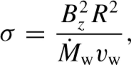
where is the mass outflow rate in the wind. Note that σ increases as the square of spherical radius (R) so that, even if B_z is very small, magnetic forces will always be important at some distance.

When the expanding shell of shocked material reaches a radius at which σ is near unity, the shell will deviate from spherical symmetry. The cylindrical r component of the wind velocity will be forced to zero. Since the wind travels faster than any information-carrying waves, the deceleration of the wind will be in the form of a shock. Pressure forces behind the shock will channel the post-shock flow toward the axis. The location of the deceleration shock in the equatorial plane is determined by setting σ= 1 in equation (2) and solving for R. Our simulations (presented in Sections 2.1 and 2.2) agree with this prediction for various wind and ambient parameters subject to condition 1.

2.1 MHD simulations

To test the simple concept of an isotropic central wind interacting with a constant vertical field, and to develop insight into more complex problems, we have carried out a number of numerical simulations. We use the 2.5D MHD code of Matt et al. (2002), and the reader will find the details there (see also Goodson, Winglee & Böhm 1997; Matt 2002). The simulations employ a two-step Lax–Wendroff (finite-difference) scheme to solve the ideal MHD equations on a series of nested boxes. The equations allow for an ideal gas equation of state (γ= 5/3) and assume that the system is axisymmetric (∂/∂φ= 0 for all quantities). Each box consists of a 101 × 100 cylindrical (r-z) grid with constant grid spacing. The boxes are nested concentrically, so that the inner box represents the smallest domain at the highest resolution. The next outer box represents twice the domain size with half the spatial resolution (and so on for other boxes). For the simplified approach of this section, we use five boxes and ignore the effects of gravity and magnetic diffusion. Outflow boundary conditions (all variables are continuous) exist on the right and top boundary of the outermost box, allowing material to leave the box without reflecting information inward.

The wind source is a multiple layered boundary, consisting of a circle with an outer radius of 10.5 grid points in the smallest box, centred on the origin of the grid. The boundary conditions on the wind sphere are as follows. All quantities are fixed (velocity = 0.0, B= 0.0, and density and pressure are constant) for R≤ 8.5 (R= (r²+z²)^1/2). For 8.5 < R≤ 9.5, the same is true except that B floats (i.e. it evolves naturally in the course of the simulations). For 9.5 < R≤ 10.5, the velocity is fixed at a constant, non-zero value and is directed radially, while all other quantities are the same as for 8.5 < R≤ 9.5. The existence of a layer with a zero velocity and a floating B interior to a layer with non-zero velocity is necessary to preserve ∇·B= 0 near the wind source boundary (similar conditions are used by Matt et al. 2000). The wind source in the simulations represents a reference surface far from the region where the wind is accelerated. In this way, the fact that the wind is supersonic and super-Alfvénic and the neglect of gravity is justified.

The grid initially has a constant density, pressure, B_z, and zero velocity. The key parameter is σ_*, where the asterisk subscript refers to the value at the radius of our wind source, defined by . At t= 0, the wind begins to move outward from the wind source, pushing the ambient material ahead of it and sweeping up the ambient magnetic field. We first verified that, when B_z= 0 (σ_*= 0), the resulting WBB is spherically symmetric. Nine other cases, with finite B_z, were sufficient to cover a range of parameters. Table 1 contains the parameter values of each case, and the simulation results are the topic of the next section. We consider the case with σ_*= 0.0087, ratio of wind source density to ambient density (ρ_*/ρ_a) = 10, wind Mach number (v_w/c_s,w) = 5, and ratio of ambient Alfvén speed to sound speed (v_A,a/c_s,a) = 5, as our baseline, with which to compare all other simulations.

Table 1.

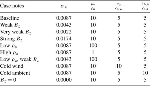
Isotropic wind simulation parameters.

Open in new tabDownload slide

2.2 Results

In the very earliest stage of the simulations, the interaction between the wind and the stagnant environment produces an expanding, spherically symmetric WBB. The flow has the following important features:

• (i)

  an interior filled with free-flowing wind;

• (ii)

  a reverse shock (RS), where wind kinetic energy is converted into thermal energy;

• (iii)

  a contact discontinuity (CD) separating the shock-heated wind gas from the shock-heated ambient gas; and

• (iv)

  a forward shock where the expanding structure runs into ambient material and heats it.

As the simulation evolves, and the structure expands, the vertical magnetic field (B_z) in the ambient material is swept aside in r. When the WBB reaches a location where σ (equation 2) is near unity, the RS slows and eventually stagnates. The position of the CD on the equatorial plane also stops, and pressure gradients in the region between the RS and CD channel material toward the axis. The end result is a steady-state, collimated flow (a jet) propagating along the z-axis.

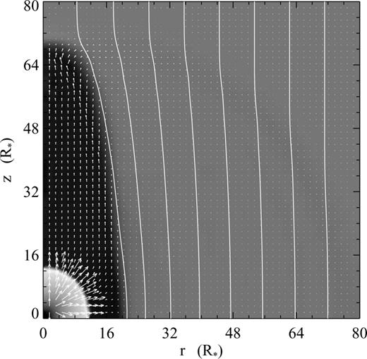
Fig. 1 illustrates the flow for the baseline case near steady-state, within 40 wind-source radii. The figure clearly demonstrates the existence of a RS at about 12R_* (where the velocity of the wind suddenly drops) and the channeling via pressure gradients of the post-shock flow toward the axis. The deflected and compressed field lines (near the CD) provide a J×B force that balances the dynamic pressure of the wind. Fig. 1 confirms the conceptual model of Kwan & Tademaru (1988, compare with their fig. 2).

Figure 1.

Grey-scale image of log density (darker is higher density), field lines and velocity vectors illustrate the near steady-state flow for the σ_*= 0.0087, baseline case.

Open in new tabDownload slide

We plot the equatorial stagnation location of the RS in seven of our simulations, as a function of the parameter σ_*, in Fig. 2. Square symbols represent the four cases with baseline ambient density (top four rows in Table 1), though each include a unique value of B_z. The triangles represent two cases with the ambient density decreased by a factor of 10 (rows 5 and 7 of Table 1), and the diamond is for the case with increased ambient density (row 6). We did not plot the results for the two simulations with various wind and ambient temperatures (rows 8 and 9), since they were indistinguishable from the baseline case. The error bars in Fig. 2 represent the uncertainty due to the finite width of the shock, caused mainly by the relatively low numerical resolution. The dotted line represents the radial location where σ= 1.0 for each σ_*. Fig. 2 demonstrates that, within the uncertainty, the location of the RS on the equator is indeed predicted by equation (2).

Figure 2.

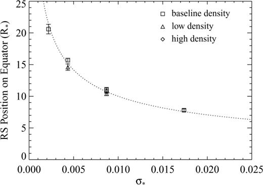
Equatorial location of the standing, star-facing shock as a function of σ_*. The simulated data (symbols for various cases indicated on figure) agree with the analytical prediction (dotted line). The errors in the simulated values (vertical bars) are due to the finite width of the standing shock (due to numerical resolution).

Open in new tabDownload slide

Fig. 3 is a grey-scale image of the pressure (logarithmic) for the baseline case. The data are from the same time as in Fig. 1, but they represent the next outer box. The figure demonstrates the propagation of the jet along the axis. The jet is composed of shocked gas, and it is supported laterally by the balance of internal thermal pressure versus external magnetic forces. The outer edge of this jet (i.e. the edge of the high-pressure region) represents the CD and is thus the location of the expanding bubble studied by (e.g.) Stone & Norman (1992). Though the jet propagates at a velocity that is higher than c_s,a and comparable to v_A,a, it is travelling slower than its own internal sound speed. In the more general case of an anisotropic central wind, it is possible for the shocked gas (the jet) to travel faster than its own internal sound speed. Also, if the gas were allowed to cool radiatively, the jet structure would be different.

Figure 3.

Grey-scale image of log pressure (darker is higher pressure), field lines and velocity vectors illustrate the flow at a late time and a larger scale for the σ_*= 0.0087, baseline case shown in Fig. 1.

Open in new tabDownload slide

Since the flow is subsonic between the RS and CD, the pressure is roughly constant and equal to the decrease in the wind dynamic pressure across the RS (i.e. the kinetic energy in front of the shock is converted to thermal energy behind it). This is evident in Fig. 3. The thermal pressure of the shocked wind extends the influence of the wind dynamic pressure to larger radii. The width of this extension on the equator (equal to the distance between the RS and the CD) depends upon how fast the shocked wind is moved toward the axis by small pressure gradients, which depends on how fast the material on the axis flows away (i.e. the speed of the jet).

For given wind parameters and B_z, the jet speed is determined by the conditions (in particular, the Alfvén speed; see Levy 1971) in the ambient medium. The ambient density, ρ_a, is important, since it behaves as an inertial barrier to the jet and it determines the Alfvén speed. For a smaller ρ_a, the jet moves faster, allowing the equatorial region between the RS and CD to be ‘drained’ more quickly by pressure gradients. Fig. 4 shows the case that is identical to the baseline case but with an ambient density decreased by a factor of 10 (row 5 of Table 1). The figure depicts an earlier time than Fig. 1 because the jet moves more rapidly toward the top of the outer box (which limits the length of time the simulations can run), but a steady state already exists within about 20 wind sphere radii. A comparison between Figs 1 and 4 reveals a dependence of the CD location (equivalent to where the magnetic field jumps in value) on the ambient density.

Figure 4.

Grey-scale image of log density (same grey-scale as Fig. 1), field lines and velocity vectors illustrate the flow at near steady-state for the σ_*= 0.0087 case with ambient density a factor of 10 less than the baseline case (Figs 1 and 3).

Open in new tabDownload slide

The relationship between the CD location and ρ_a is even more apparent in Fig. 5, a plot of the CD location versus the parameter σ_*. The symbols represent the same cases as in Fig. 2, and the dotted lines represent the radii of various values of σ as a function of σ_*. For the cases of any given ambient density, the points follow the same trend (though shifted in position) as for the location of the RS. For an increased ambient density, the steady-state location of the CD on the equator moves outward.

Figure 5.

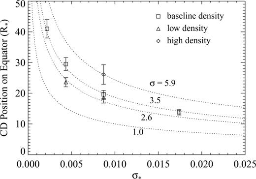
Equatorial location of the jump in B_z as a function of σ_*. The simulated data (symbols for various cases indicated on figure) follow the predicted trend for the standing shock (dotted lines for different values of σ, chosen to fit the data) but also reveal a dependence on conditions of the ambient material. The errors in the simulated values (vertical bars) are due to the finite width of the jump in B_z (due mainly to numerical resolution).

Open in new tabDownload slide

3 Collimation of A Yso Outflow

In this section we consider the more complex case of an anisotropic wind collimated by an initially vertical magnetic field embedded in an accretion disc. It is our goal to compare these results to observations of outflows from YSOs, so we adopt a central wind launching mechanism that is appropriate for those systems. In the absence of any disc field, this MHD mechanism (reviewed in Section 3.1) produces an outflow with a collimated (jet) component plus an uncollimated wind. Both components of the flow are relatively fast (100–200 km s⁻¹) and of the order of the Keplerian rotation speed at the central region from which the wind is launched. Our simulations (described in Section 3.2 and results presented in Section 3.3) resolve the detailed launching of the central wind, and they will show that a large-scale field, embedded in the accretion disc, will collimate the wide-angle component of the wind. This results in a more powerful and physically broader jet than that produced in the absence of the disc field. We also show that the simple results of the last section hold, even for the more complex outflow morphologies produced in this section.

For simplicity, we will assume an initially constant, vertical field frozen into the disc and permeating an environment above and below the disc that is initially in hydrostatic equilibrium. The small time-scales involved in properly capturing the launching of the central wind make it impractical for us to follow also the launching of disc plasma along the initially vertical field lines. Therefore, the existence of a wide-angle, slow, disc wind observed in some systems (Kwan & Tademaru 1988) is not addressed by our models. Such a wind may result from, or be responsible for, the existence of a large-scale, primarily vertical magnetic field (assuming it is sufficiently ionized; e.g. Blandford & Payne 1982). Our simple treatment of the disc field will, in some ways, emulate a magnetized disc wind that can act as a channel for the interior, wide-angle wind (e.g. Ouyed & Pudritz 1997). We propose that the relatively broad jet, produced by the collimation of a central wind by this disc field, can explain some of the observational properties (e.g. the mass flux, velocity, energy and momentum budget, and collimation) of optical jets.

3.1 The central wind

For the central wind, we adopt a model studied by Hayashi, Shibata & Matsumoto (1996), Goodson et al. (1997), and Miller & Stone (1997), in which a rotating star couples to the inner edge of a conductive accretion disc via a stellar dipole magnetic field. In this model, differential rotation between the star and disc twists up the magnetic field, adding a B_φ component. The magnetic pressure associated with B_φ causes the stellar magnetosphere to expand (or ‘inflate’) above and below the disc. Plasma loaded onto the inflating field lines is driven outward in a burst. When the inflation speed becomes larger than any plasma wave speeds, the field lines become effectively open, and material is magnetocentrifugally launched from the disc inner edge via the Blandford–Payne mechanism (Blandford & Payne 1982). Plasma launched from the inner edge of the disc carries away angular momentum, so the disc spins down and moves inward. The inward motion of the disc forces together the open field lines from the star and disc of opposite polarity, instigating a reconnection of those lines. After reconnection, material at the disc inner edge is again magnetically coupled to the star, but with less angular momentum than before, so that it accretes via funnel flow along field lines onto the star. The accretion of material unloads the stellar magnetosphere, allowing it to expand outward and diffuse into the new inner edge of the disc. When the field begins to thread the disc inner edge, differential rotation again twists up the field, and the process repeats. This process of episodic magnetospheric inflation (EMI) regulates both the accretion and ejection of material within the region of the disc inner edge.

By following the outflow to several au, Goodson et al. (1997) and Goodson, Böhm & Winglee (1999) showed that the EMI mechanism produces a jet (hereafter, the ‘EMI jet’) that has knots associated with each reconnection event. Note that the typical oscillation period for the EMI mechanism is about 20–30 d, too short to explain the knot spacing in observed jets (e.g. in HH 30; Burrows et al. 1996). The rest of the flow travels out at a wide opening angle, shocking the surface of a flared accretion disc. The flow speed for the EMI jet and wide-angle wind component is ≳100 km s⁻¹, in rough agreement with observations (Reipurth & Bally 2001). The energetics and the mass outflow rate in the EMI wind are also within the range observed in jets, but most of the kinetic energy and mass in the EMI wind is contained in the wide-angle component (not in the jet). In addition, the width of the EMI jet component is a few au, an order of magnitude smaller than observed (e.g. Burrows et al. 1996).

In their limited parameter study of the EMI mechanism, Matt et al. (2002) showed that a weak magnetic field, aligned with the rotation axis and threading the accretion disc, did not affect the launching of the EMI outflow. This should be true, as long as the stellar dipole field is stronger than the vertical field at the inner edge of the disc. Their work focused on the integrated outflow properties, rather than the details of the wind morphology, and they were unable to address the collimation of the outflow by the vertical fields because the size of their largest simulation grid reached only to 0.75 au. In this section, we follow up the work of Matt et al. (2002) and, using insight gained from Section 2, we will show that when one follows the outflow to large enough distances, even a weak field will collimate the entire EMI outflow.

Many other authors (e.g. Shu et al. 1994; Lovelace, Romanova & Bisnovatyi-Kogan 1995; Fendt & Elstner 1999; Küker, Henning & Rüdiger) have discussed outflows produced by the interaction between a stellar magnetosphere and the inner edge of the disc. The EMI mechanism operates only when the magnetic diffusivity is relatively small in these systems (Goodson & Winglee 1999), but the outflows produced in all of these studies contains a component that flows out at wide angles. We choose to work with the EMI model as one example, but our conclusions apply to any wide-angle, central flow.

3.2 Simulation method

As in Section 2, we use the 2.5D MHD code of Matt et al. (2002). For the more complex simulations carried out in this section, the code solves the ideal MHD equations with the added physics (via source terms in the momentum, energy, and induction equations) of gravity and ohmic diffusion. We also adopt their baseline simulation case, in which a 1 M_⊙, 1.5 R_⊙ T-Tauri star with a 1.8-d rotation period interacts with a flared accretion disc (after the α-disc model of Shakura & Sunyaev 1973) via an axis-aligned dipole magnetic field (= 909 G on the equator). The reader will find more details of the simulations and initial conditions in Matt et al. (2002) and Goodson et al. (1997, 1999). Our simulations differ from those of Matt et al. (2002) only in that we use 10 nested boxes, while they used only four. Each simulation box consists of a 401 × 100 cylindrical (r-z) grid, and the boxes are nested concentrically (see Section 2.1). In this way, we fully capture the launching of the outflow via the EMI mechanism in the innermost box, while our outermost box follows the flow out to 24 au.

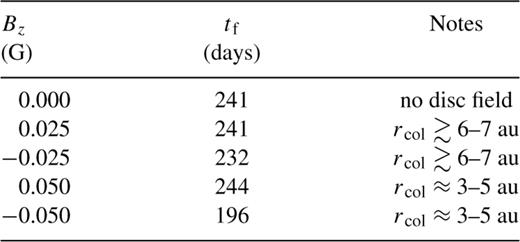
First, we simulated the baseline case and followed the outflow to large radii, allowable by the increased number of boxes. We then ran four other cases with an additional vertical and constant magnetic field (B_z) initialized everywhere in the simulation region. All of the cases are identical except for the strength of the initial vertical field. So the baseline case has B_z= 0, and the others have |B_z|= 0.050, or 0.025 G. The vertical field can interact (e.g. reconnect) with the field carried in the outflow, so there is a need to assess the effect of polarity of the vertical field. Thus, for each case with non-zero |B_z|, we ran two cases, each with opposite polarity. Table 2 lists the values of B_z, the simulation time at which the simulations were stopped (t_f), and some notes for each case.

Table 2.

YSO simulation parameters.

Open in new tabDownload slide

Our choice of vertical field strengths was based on the need for the field to be strong enough to collimate the flow within the outer box and weak enough not to effect the EMI mechanism (which gives an upper limit of ∼0.1 G). We used equation (2) to estimate the required field.

3.3 Results

In the absence of any disc field, the basic properties of the EMI wind include:

• (i)

  a relatively high-density, narrow jet (the EMI jet) along the z-axis; and

• (ii)

  a wide-angle wind.

These features are apparent in Fig. 6, a snapshot from the tenth simulation box of the outflow in the B_z= 0 baseline case at 241 d. The star is at r=z= 0, and the data have been reflected about the r= 0 axis to demonstrate the flow better. The figure also contains data from the eighth and ninth simulation boxes, which extend to 6 and 12 au, respectively, in z. The outflow is highly structured, containing knots in the jet and ‘wispy’ structures in the wide-angle wind. These structures are correlated with oscillations of the EMI mechanism. The entire flow originates from a region of ≲30 R_⊙, where the inner edge of the disc is located. By the time of this snapshot, material originating in the disc or on the star has travelled to ∼16–18 au, and the flow at larger z is transient (i.e. due to the initial expansion into a stagnant environment).

Figure 6.

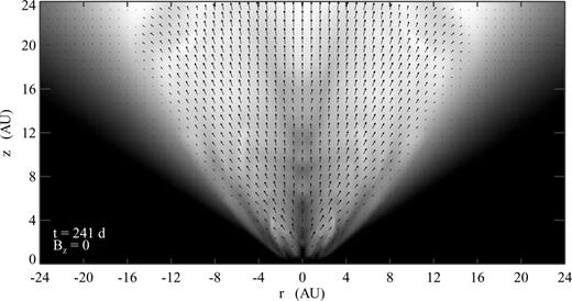
Grey-scale image of density (logarithmic) and velocity vectors from the case with no vertical field at 241 d. Log ρ > −15.3 gm cm⁻³ is black; log ρ < −19.3 gm cm⁻³ is white.

Open in new tabDownload slide

Fig. 7 is a snapshot from the B_z= 0.025 G (left panel) and B_z=−0.025 G (right panel) cases at 241 and 232 days, respectively. It is evident that the wide-angle flow has been completely collimated by the disc-associated field to a width of 6–7 au. In other words, the EMI jet and wide-angle wind have been combined into a broad, collimated structure (hereafter, the ‘broad jet’). Note that the narrow EMI jet is still apparent along the axis, and a relatively dense shell has formed on the outer edge (in r) of the broad jet, where material travelling at large polar angles piles up against the disc field before changing direction. However, the central EMI jet and the outer shell exists only to a height that is comparable to the collimation height of the broad jet (at z≈ 12 au). A comparison between the left and right panels of Fig. 7 reveals that there is almost no difference in collimation radius for the cases with opposite disc field polarity. As in Fig. 6, the main flow has reached to z∼ 16–18 au. Since this distance is comparable to the width of the broad jet, the final collimation width may become a little larger than that achieved by the time of this snapshot.

Figure 7.

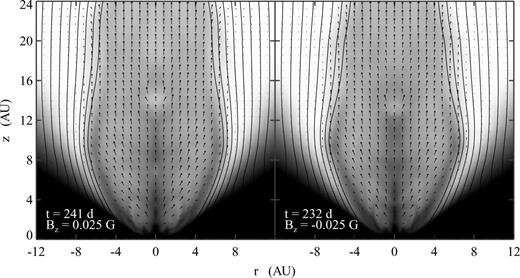
Grey-scale images of density (logarithmic), magnetic field lines and velocity vectors from the case with a 0.025 G vertical field. The two panels represent simulations that are identical except for the polarity of the vertical field (left panel has positive B_z, the right has negative, and the time in days is shown in each panel). The grey-scale is identical to Fig. 6, and the line spacing is proportional to field strength.

Open in new tabDownload slide

Fig. 8 is a snapshot from the B_z= 0.05 G (left panel) and B_z=−0.05 G (right panel) cases at 244 and 196 days, respectively. This figure shows the collimation of the entire central flow to a width of 3–5 au. Again, the two panels show that there is almost no difference in collimation radius between the two cases of opposite disc field polarity. As in Fig. 7, both panels also contain the central EMI jet and a dense shell enclosing the broad jet to a height of z≈ 8 au, where the broad jet becomes collimated.

Figure 8.

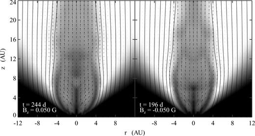
Grey-scale images of density (logarithmic), magnetic field lines and velocity vectors from the case with a 0.05 G vertical field. The two panels represent simulations that are identical except for the polarity of the vertical field (the left panel has positive B_z, the right has negative, and the time in days is shown in each panel). The grey-scale is identical to Fig. 6, and the line spacing is proportional to field strength.

Open in new tabDownload slide

The data plotted in Figs 7 and 8 are consistent with the prediction of equation (2) that the collimation radius is inversely proportional to the disc field strength. For a more quantitative analysis, we plot various outflow properties as a function of polar angle (θ) at a constant spherical radius in Figs 9–11. Because the wind is episodic and highly structured, and because our time sampling for data outputs is fairly course (2.8 d), it is necessary to represent the outflow properties as time-averaged quantities that cover several periods of the EMI oscillation (which is around 20–30 d). We therefore calculate the outflow quantities for each case at 90 grid points out in our eighth simulation box (= 5.4 au) and average them from 112 d until the end of the simulation.

Figure 9.

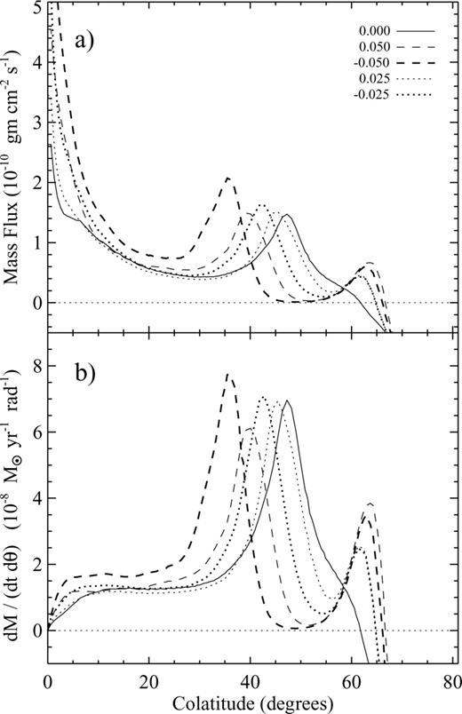
(a) Time-averaged mass flux and (b) time-averaged mass outflow rate per radian (, see text) versus polar angle, at a constant radius of 5.4 au. The solid line in each panel represents the case without a vertical field (B_z= 0), the dotted lines are for cases with |B_z|= 0.025 G, and the dashed lines are for cases with |B_z|= 0.05 G. Bold lines are for B_z < 0, and the lighter lines are for B_z > 0.

Open in new tabDownload slide

Figure 10.

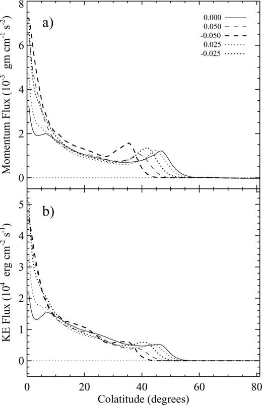
(a) Time-averaged linear momentum flux and (b) time-averaged kinetic energy flux versus polar angle, at a constant radius of 5.4 au. The line styles represent the same cases as in Fig. 9.

Open in new tabDownload slide

Figure 11.

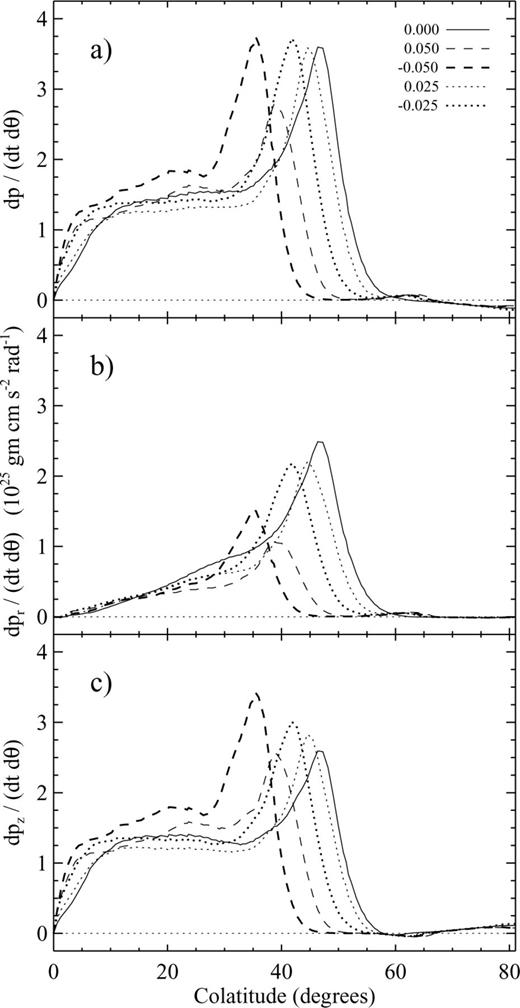
Time-averaged momentum outflow rate (thrust) per radian (, see text) for (a) the total, poloidal momentum, (b) the radial component, and (c) the vertical component versus polar angle, at a constant radius of 5.4 au. All three panels are plotted on the same scale. The line styles represent the same cases as in Fig. 9.

Open in new tabDownload slide

Fig. 9(a) shows the mass flux, Φ_M (θ), for all cases. The existence of the narrow EMI jet at θ≲10° is represented by the strongly peaked mass flux there for all cases. Note that, for θ≳ 65°, Φ_M becomes negative, as this represents material inside the accretion disc. Fig. 9(b) shows the mass outflow rate per differential polar angle; , where R is the spherical radius. It is evident that, while Φ_M is greatest near the pole, most of the mass in the flow exists at large opening angles (θ > 25°). For every case, there is a peak in Φ_M and where θ is between 25° and 55°. For larger B_z, this peak is deflected to smaller angles. The wide-angle flow is not completely collimated at z= 5.4 au for any of the cases (see Figs 7 and 8), but the deflection of this peak indicates the onset of collimation. The cases with positive B_z are shifted a few degrees less than their negative B_z counterparts. A positive and negative B_z corresponds to the stellar magnetosphere having an initially open and initially closed topology, respectively (see Matt et al. 2002). This suggests that the open topology is slightly less efficient at collimating at 5.4 au (presumably due to the release of magnetic energy from magnetic reconnection between disc field lines and those carried in the outflow), though the final collimation radius is not much affected by the topology of the field (as evident in Figs 7 and 8). Finally, there is a bump in Φ_M between 55° and 65° for the cases with |B_z| > 0. This feature is much less prominent in the momentum and kinetic energy (see Figs 10 and 11) of the outflow, indicating that it has relatively high density and low velocity compared to the rest of the outflow. It represents material being pushed aside by the compression of disc field lines.

The total mass outflow rate can be obtained by integrating over a desired range of θ. For all cases, the positive mass outflow rate (excluding the bump at 55° < θ < 65° for the |B_z| > 0 cases) is ∼1.5–2.0 × 10⁻⁸ M_⊙ yr⁻¹ in one hemisphere. This agrees very well with the typical value of yr⁻¹ derived from observations of jets (Reipurth & Bally 2001). Note, however, that for the B_z= 0 case, the mass loss happens toward large opening angles, while for the |B_z| > 0 cases, the whole of is contained in the broad jet.

All cases also show a very strongly peaked EMI jet in the momentum flux (Fig. 10a), , and kinetic energy flux (Fig. 10b), . The total kinetic energy outflow rate (mechanical luminosity) of the flow is ∼10³² erg s⁻¹, lower than the typical value of ∼1 L_⊙ reported by Reipurth & Bally (2001). The wide-angle peak in both fluxes of Fig. 10 follows the same case-by-case behaviour as in Fig. 9. That is, the peak shifts to smaller angles for stronger |B_z|.

Fig. 11 shows the linear momentum outflow rate (thrust) per differential polar angle; -flux(θ), where p_x is m(v²_r+v²_z)^1/2 for Fig. 11a, mv_r for Fig. 11b, and mv_z for Fig. 11c. The total vertical momentum outflow rate (Fig. 11c) is ∼10²⁵ dynes for all cases, lower than the typical value of ∼10²⁶ gm cm s⁻², reported by Reipurth & Bally (2001). In all cases, the total thrust (Fig. 11a) is dominated by the vertical thrust (Fig. 11c) for θ≲ 40°. For the baseline case, the r-directed (Fig. 11b) and vertical thrust (Fig. 11c) are comparable for θ≳ 40°, indicating that the flow is moving in a direction of ∼45° there. This is because the wide-angle component of the B_z= 0 case is not collimated. However, Fig. 11b demonstrates that, for increasing |B_z|, the total r-directed thrust decreases. This is because the expanding wind experiences a negative-r-directed J×B force from the perturbed disc field. The peak in vertical thrust (c) shifts to smaller polar angles for larger |B_z| (indicating the onset of collimation), but the total vertical thrust (integrated over θ) is roughly the same for all cases.

The calculation of the outflow thrust (Fig. 11) allows us to apply the results of Section 2 quantitatively, though roughly, to the EMI outflow. Since it is only the r-directed component of the wind that deflects the disc field before the collimation radius is reached, we will replace of equation (2) with and set σ equal to unity. The collimation radius can then be estimated as

(3)

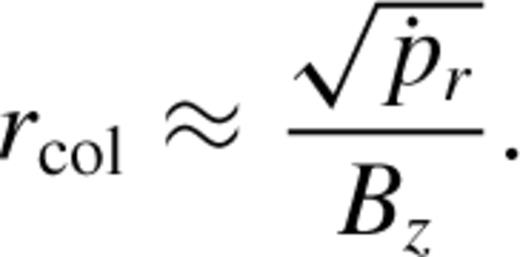
The (integrated over θ) for the B_z= 0 case is ∼6.5 × 10²⁴ dynes in one hemisphere. This predicts a r_col of 4.8 and 9.6 au for the |B_z|= 0.05 and 0.025 G cases, respectively. This prediction is slightly larger than the simulated value for the |B_z|= 0.025 cases (see Fig. 7 and Table 2), but remember that the simulated flow in that case has not quite reached its full collimation radius. Also, for a magnetized central wind (as in the EMI outflow), there will be an increase in the collimation (decrease in r_col) as B_φ carried in the wind is compressed in the outer shell (see Figs 7 and 8; Gardiner et al. 2003).

4 Summary and Discussion

The relatively high velocity of observed YSO jets requires that jet material is launched from deep within the gravitational potential well (i.e. within several stellar radii). In order to explain the observed jet widths and their degree of collimation, the jet material must be launched initially with wide opening angle and become almost completely collimated at a distance from the star that is comparable to the width of the jet. Self-collimation of the wide-angle wind (due to magnetic fields carried in the wind itself) cannot occur for 100 per cent of the wind material; there is always some material leaving at very wide angles. This argues for the existence of a collimator that is external to the central wind. We have explored one such possibility.

Specifically, we used time-dependent MHD simulations to extend the work of Kwan & Tademaru (1988) and demonstrate that any outflow (even if initially isotropic) will be eventually collimated by a constant, parallel magnetic field of any strength. The collimation of the central wind is inevitable, assuming that the wind is sufficiently ionized to interact with the field. This is because the ram pressure in the wind always decreases with radius for a diverging wind, and the magnetic pressure is constant. The collimation radius is roughly given by the location where the two energy densities balance.

In Section 3, we applied this concept to realistic YSO outflows by first adopting the episodic magnetospheric inflation (EMI) model (Hayashi et al. 1996; Goodson et al. 1997, 1999; Miller & Stone 1997) for launching the outflows. We then assumed that the entire simulation region was initially threaded by a vertical magnetic field. The result is that the wide-angle component of the EMI wind is collimated by disc fields of ≪0.1 G. In this way, the entire mass, momentum, and energy budget of the central outflow is channelled into a relatively fast (100–200 km s⁻¹), broad jet with a width of several au. The channelling occurs within a vertical height of the order of the jet width, consistent with observational constraints (see Section 1).

The morphology of the resulting broad jet includes a relatively narrow density enhancement along the axis. This feature is the narrow jet produced by the EMI mechanism alone (i.e. even when there is no disc field). The collimation of the wide-angle wind results in a relatively high-density shell of shocked, outflowing material surrounding the flow out to at least the height of collimation. The EMI jet and shocked shell together resemble a ‘pitchfork’ in projection (see Figs 7 and 8).

Bally, Feigelson & Reipurth (2003) recently suggested that X-ray emission from a region 0.5–1.0 arcsec west-southwest of the YSO L1551 IRS 5 may be explained by shocks associated with the collimation of the main outflow from that region. Using kinematic information from infrared slit observations of that outflow, Pyo et al. (2002) demonstrated the existence of two different flows (not including the molecular outflow discovered by Snell, Loren & Plambeck 1980): an ionized, highly collimated jet moving at ∼440 km s⁻¹, and a partially ionized, wide-angle wind moving at ∼200 km s⁻¹. The wide-angle wind shows a kinematic signature of increased collimation as it moves further from the source. Pyo et al. (2002) also noted a pitchfork-like morphology in an I band image of the outflow, which they suggested could represent the limb-brightened edges of the wide-angle wind under collimation. Note, however, that the southernmost of the pitchfork ‘tines’ has been interpreted as a separate jet from a companion star (Fridlund & Liseau 1998; Hartigan et al. 2000).

In this paper, we have assumed the special geometry of an axis-aligned, vertical field, which requires that the field is associated with the accretion disc. This field could represent a field carried in a disc wind (moving more slowly than the central wind), though we don't follow such a wind in our simulations. Specifically, if the disc is magnetized, and if there is a magnetized outflow from the disc, the field will roughly follow the wind streamlines in the poloidal plane. Indeed, the predicted poloidal field geometry for disc wind-launching models (e.g. Uchida & Shibata 1985; Shibata & Uchida 1986, 1990; Ouyed & Pudritz 1997; Ustyugova et al. 1999) is essentially vertical near the rotation axis.

Disc wind models also predict that the field has a helical structure, due to the winding up of field lines by the rotation of the disc. The azimuthal field, added in this way, increases the collimation of the disc wind (Blandford & Payne 1982; Sakurai 1985), and would therefore further constrain any central, wide-angle flow that interacts with it. Due to the long time-scale for the winding of the disc field compared to the time-scale for the launching and propagation of the central wind by the EMI mechanism, our simulations do not capture the effect of the azimuthal component expected in the disc-associated field.

Also, due to differential rotation and possibly turbulence in a real accretion disc, it is reasonable to assume that any field present in the disc may be disordered, and possibly chaotic (e.g. Blandford & Payne 1982; Hawley & Balbus 1992). A disc wind would therefore be threaded by a magnetic field with direction reversals at irregular intervals (i.e. flux tubes with opposite polarity). Such direction reversals do not affect the qualitative behaviour of the field (see, e.g. Tsinganos & Bogovalov 2000). That is, whether the vertical field has a constant or chaotic polarity, it will always act to collimate the flow (see also Li 2002, for a similar description with a chaotic field).

The interaction of a wide-angle wind with an external, disc-associated magnetic field (as presented here) is not the only possible large-scale collimation mechanism for YSO outflows. A few authors (Frank & Noriega-Crespo 1994; Frank & Mellema 1996; Li & Shu 1996; Mellema & Frank 1997; Delamarter, Frank & Hartmann 2000; Gardiner et al. 2003) have discussed the interaction of wide-angle flows with an unmagnetized environment (see also Lery et al. 2002). They have found that the wide winds may be completely collimated by shock focusing, especially when azimuthal magnetic fields are present in the wide-angle wind. It is not clear what the observational signature of such an interaction would be (for possible detections, see Bally et al. 2003; Matt & Böhm 2003), but it takes place relatively close to the source and therefore may be difficult to disentangle from the complex emitting environment there.

Acknowledgments

This research was supported by NSF grant AST-9729096 and by the National Science and Engineering Research Council of Canada (NSERC), McMaster University, and the Canadian Institute for Theoretical Astrophysics through a CITA National Fellowship.

References