


Abstract
We discuss the evolution of the magnetic field of an accreting white dwarf. We calculate the ohmic decay modes for accreting white dwarfs, the interiors of which are maintained in a liquid state by compressional heating. We show that the lowest-order ohmic decay time is (8–12)×109 yr for a dipole field, and (4–6)×109 yr for a quadrupole field. We then compare the time-scales for ohmic diffusion and accretion at different depths in the star, and for a simplified field structure and assuming spherical accretion, study the time-dependent evolution of the global magnetic field at different accretion rates. We neglect mass loss by classical nova explosions and assume that the white dwarf mass increases with time. In this case, the field structure in the outer layers of the white dwarf is modified significantly for accretion rates above the critical rate M·c≈(1–5)×10-10 M⊙ yr-1. We consider the implications of our results for observed systems. We propose that accretion-induced magnetic field changes are the missing evolutionary link between AM Her systems and intermediate polars. The shorter ohmic decay time for accreting white dwarfs provides a partial explanation of the lack of accreting systems with ≈109 G fields. In rapidly accreting systems such as supersoft X-ray sources, amplification of internal fields by compression may be important for type Ia supernova ignition and explosion. Finally, spreading matter in the polar cap may induce complexity in the surface magnetic field, and explain why the more strongly accreting pole in AM Her systems has a weaker field. We conclude with speculations concerning the field evolution when classical nova explosions cause the white dwarf mass to decrease with time.
1 Introduction
There are now ∼65 isolated magnetic white dwarfs known, and a further 90 accreting magnetic white dwarfs (WDs) (see Wickramasinghe & Ferrario 2000, hereafter WF, for a recent review). Interesting differences are emerging between the isolated and accreting populations. Measured field strengths of the isolated WDs range from 3×10⁴ to 109 G, whereas the range of field strengths of accreting WDs may be smaller. The magnetic field strengths in the AM Her binaries are measured directly to be in the range 107–2×10⁸ G, and the magnetic fields of the intermediate polars (IPs) are inferred to range from 107 down to ≈105 G. The observed fraction of magnetic systems is 5 per cent for isolated WDs, but 25 per cent for accreting systems. There is evidence that isolated magnetic white dwarfs are more massive than the typical 0.6-M⊙ non-magnetic WDs, with a mean mass ≳0.95 M⊙. Measurements of accreting magnetic white dwarfs, however, give masses ≈0.7 M⊙, consistent with the measured masses of non-magnetic (B≲105 G) accretors. One similarity between isolated and accreting WDs is that the magnetic field is often seen to be complex, with a significant quadrupole (or offset dipole) component.
The origin and evolution of white dwarf magnetism is an important, but as yet unsolved, part of our understanding of stellar evolution. Several papers have discussed the evolution of magnetic fields in isolated, cooling white dwarfs. Ohmic decay of magnetic fields was first addressed by Chanmugam & Gabriel (1972), and Fontaine, Thomas &, van Horn (1973), who showed that the decay time of the lowest-order decay eigenmodes was longer than the evolution time of the white dwarf. Wendell, van Horn & Sargent (1987, hereafter WVS) followed the evolution of different decay modes along a cooling sequence. They found that the fundamental dipole mode decayed by a factor of 2 in 1010 yr. These studies suggested that WD magnetic fields are fossil fields left over from previous evolution. For example, one proposal consistent with the high masses (≳0.95 M⊙) of magnetic white dwarfs is that they result from evolution of the strongly magnetic (102–104 G) Ap and Bp main-sequence stars. The higher-order field components decay more rapidly, however, leading Muslimov, van Horn & Wood (1995, hereafter MVW) to study the Hall effect as a way of generating field complexity during the lifetime of the white dwarf.
The result that white dwarf magnetic fields evolve only very slightly over their lifetime has been applied in almost all studies of accreting white dwarfs. For example, in evolutionary studies of magnetic cataclysmic variables, it is presumed that the magnetic field of the white dwarf does not change with time. One exception is King (1985), who applied the results of Moss (1979) to accreting systems, and suggested that meridional currents could submerge magnetic flux in the outer layers of rotating magnetic white dwarfs. It is the purpose of this paper to show that the process of accretion itself may change the surface magnetic field of an accreting white dwarf significantly.
Many authors have studied the effects of accretion on the magnetic field of accreting neutron stars. This is motivated by the idea that the rapidly rotating millisecond radio pulsars are produced by accretion, which spins up the neutron star to short periods, and perhaps causes a reduction in magnetic field strength from the 1012 G fields seen in most radio pulsars to the 108–109 G fields of the millisecond pulsars (see Bhattacharya 1995 for a review). In a recent paper, Cumming, Zweibel & Bildsten (2001, hereafter CZB) returned to the suggestion that the accretion flow screens the internal magnetic field directly (Romani 1990, 1995). They compared the time-scales for ohmic diffusion and accretion in the thin outer layers of the neutron star, and computed steady-state magnetic profiles, taking the field to be horizontal and the accreted matter to be unmagnetized. For this simplified geometry, the field was found to be strongly screened for accretion rates greater than the critical rate M·∼10-10 M⊙ yr-1, whereas at lower accretion rates, the underlying magnetic field was able to penetrate the freshly accreted material. This result fits nicely with the observation that the only weakly magnetic accreting neutron star to show its magnetic field directly (the accreting millisecond X-ray pulsar, SAX J1808.4−3658; Chakrabarty & Morgan 1998, Wijnands & van der Klis 1998) has a lower accretion rate than other systems (time-averaged M·≈10-11 M⊙ yr-1), low enough that screening would not be effective in hiding its field.
A crucial question for the evolution of accreting white dwarfs is whether the white dwarf mass increases or decreases with time. For accretion rates ≲10−7 M⊙ yr−1, the accreted hydrogen and helium burns unstably, giving rise to classical nova explosions (see, e.g., Fujimoto 1982, MacDonald 1983). The observed heavy-element enrichment of nova ejecta has been used to argue that the nova explosion excavates material from the white dwarf, so that its mass is decreasing with time (e.g. Livio & Truran 1992). However, this is a somewhat open question, both because of uncertainties in measurements of ejecta masses, and in theoretical modelling. Theoretical calculations find that mixing of extra CNO nuclei into the burning shell is needed to achieve rapid enough energy release to drive novae with rapid rise times. However, the mixing mechanism is presently unknown. Prialnik & Kovetz (1995) addressed this question with hydrodynamic simulations including diffusion, and found that the white dwarf mass decreased for M·<10-9 M⊙ yr-1, and increased for M·>10-7 M⊙ yr-1. At intermediate accretion rates, the mass loss depended on the white dwarf temperature. The accretion rates of IPs are estimated to be ∼10−9 M⊙ yr−1 (see the discussion in Section 5.1), and their core temperatures in the middle of the range considered by Prialnik & Kovetz (1995) (see Section 3.2). On the other hand, AM Her systems accrete at typical rates of ≈5×10⁻¹¹ M⊙ yr−1 (Section 5.1). Thus a range of behaviour might be expected within the population of accreting magnetic white dwarfs. The magnetic field of the white dwarf itself may affect the nova outburst, for example by enhancing mass loss in the equatorial plane (Livio, Shankar & Truran 1988, Livio 1995).
In this paper, we assume that the white dwarf mass increases with time during accretion, and study the consequences for the evolution of the white dwarf magnetic field. We leave the case of decreasing white dwarf mass for a future study. First, we show that comparing accretion and ohmic diffusion times in white dwarfs gives the same critical accretion rate M·c≈(1–5)×10-10 M⊙ yr-1 as found for neutron stars by CZB (for reasons we describe in Section 3), and then go on to calculate the evolution of the magnetic field. We show that the resulting field evolution may explain several properties of observed systems.
A complication in calculating the evolution of the magnetic field in both accreting neutron stars and white dwarfs is that the accretion flow is channelled on to the magnetic polar cap (for white dwarfs, this occurs for B≳105 G). Rather than tackle the complex problem of the subsequent spreading of matter and evolution of the magnetic field, CZB presumed that the neutron star magnetic field was buried by the accretion flow into a flattened configuration, and then used a plane-parallel model to ask what accretion rate was needed to keep the field from re-emerging by ohmic diffusion. In this paper, the simplification we make is to study the evolution of the global magnetic field under spherical accretion. The accreted matter is expected to spread away from the polar cap when the magnetic tension force no longer supports the hydrostatic pressure (e.g. Hameury et al. 1983), so that spherical accretion is a good approximation, except in a thin layer of mass  for a 0.6-M⊙ white dwarf, where B7=B/107 G is the surface field strength. We include the uncertainty of what happens in this thin spreading layer as an uncertainty in the surface boundary condition for the spherically accreting models (see the discussion in Section 4.1).
We start in Section 2 by considering ohmic decay in accreting white dwarfs, which have liquid interiors because of compressional heating by accretion. In Section 3, we compare the time-scales for ohmic decay and accretion, and relate our results to those of CZB. In Section 4, we calculate the global evolution of the field, under simplifying assumptions concerning its geometry, for different accretion rates. We relate our models to the recent calculations of Choudhuri & Konar (2002) for accreting neutron stars, which adopt a similar approach. We find that for M·>M·c, the surface field strength is reduced by accretion because ohmic diffusion is not rapid enough to allow penetration of the field into the newly accreted layers. In Section 5 we discuss the implications of our results for observed systems. In Section 6, we conclude with some speculations concerning magnetic field evolution in the alternative scenario of decreasing white dwarf mass with time. In the Appendix, we describe our calculations of electrical conductivity for arbitrary degeneracy.
2 Ohmic decay in liquid white dwarfs
In this section, we discuss ohmic decay of the magnetic field, neglecting the effects of accretion for now. In an accreting white dwarf, compressional heating of the core results in a central temperature ≳107 K (Nomoto 1982), so that the interior is kept in a liquid state. In that case, the electrical conductivity is independent of temperature, allowing us to use simple zero-temperature white dwarf models. We calculate the ohmic decay modes following the original work of Chanmugam & Gabriel (1972), Fontaine et al. (1973) and WVS. We show that the lowest-order decay mode has a decay time of ≈(8–12)×109 yr, depending on the white dwarf mass.
2.1 Electrical conductivity and decay time
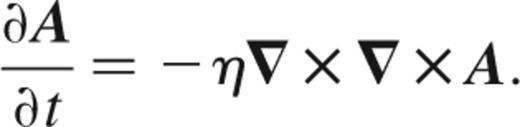
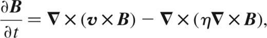
Ohmic decay is described by the induction equation
where η=c2/4πσ is the magnetic diffusivity and σ is the electrical conductivity. The associated characteristic decay time-scale is ≈4πσL2/c2, where L is the length-scale over which B changes.
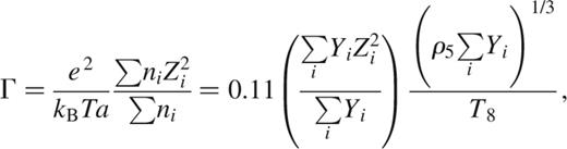
Compressional heating maintains the interior of most accreting white dwarfs in a liquid state. The melting temperature Tmelt is determined by the condition Γ≈173 (e.g. Farouki & Hamaguchi 1993), where Γ=(Ze)2/kBTa measures the ratio of Coulomb to thermal energy. For simplicity, we write Γ for a single species of ion with charge Z, mass A and interion spacing a, giving
Compressional heating gives core temperatures ≳107 K>Tmelt (Nomoto 1982), thus we expect most accreting white dwarfs to have liquid interiors. It is possible that some massive white dwarfs with central densities ≳108 g cm−3 accreting at low enough rates have solid cores, but we do not consider these systems here.
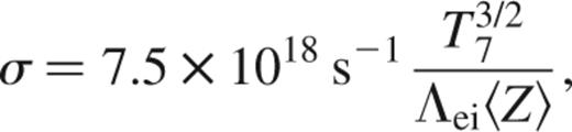
The electrical conductivity in the liquid interior is set by collisions between the degenerate electrons and the non-degenerate ions. The conductivity is
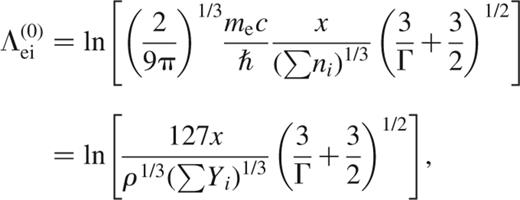
(e.g. Yakovlev & Urpin 1980, Itoh et al. 1983, Schatz et al. 1999), where x=pF/mec measures the Fermi momentum pF of the electrons, Λei≈1 is the Coulomb logarithm and 〈Z〉 is a measure of the mean nuclear charge, given by  , where Zi is the nuclear charge, Ai the mass and Xi the mass fraction of species i, and μe the mean molecular weight per electron. In terms of x, the density is ρ=1.9×10⁶ g cm-3x3(μe/2).
The fact that conductivity is independent of temperature allows us to adopt simple zero-temperature white dwarf models. In the outer envelope, where the electrons are non-degenerate, the conductivity is temperature-dependent. In the Appendix, we describe a method for calculating the electrical conductivity for arbitrary degeneracy. However, the results of this section are insensitive to the conductivity in the outermost layers. We adopt pressure as the independent variable, and integrate the equations of hydrostatic balance and mass conservation outwards from the centre of the white dwarf for an initial choice of central density. We stop the integration once the pressure falls below some fixed fraction of the central pressure, at which point the radius and mass are well determined. We assume the composition to be an equal mixture by mass of carbon and oxygen, giving μe=2 and 〈Z〉=7.
Some properties of these zero-temperature white dwarfs are shown in Fig. 1. We show the radius, central density, central conductivity σc, and ohmic time at the centre, tohm=4πR2σc/c2, as a function of the white dwarf mass.
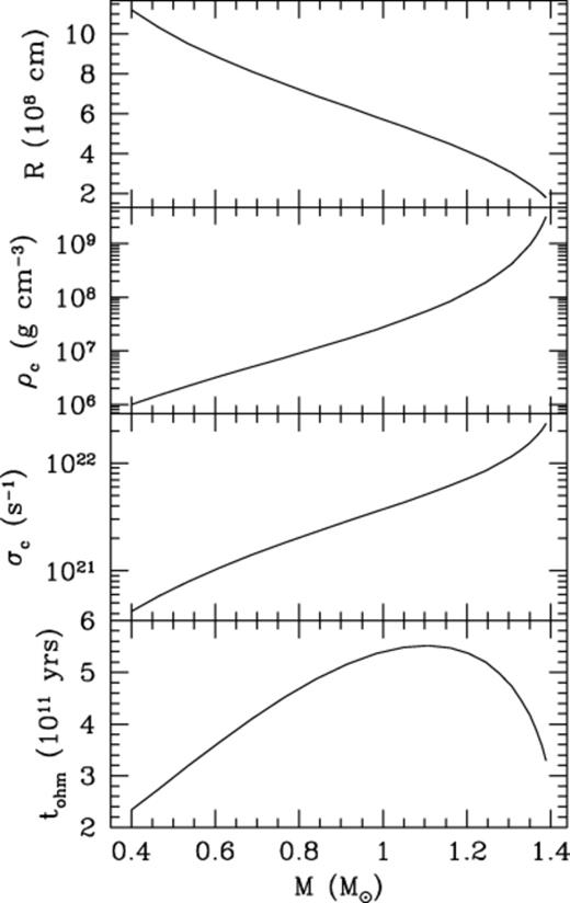
Properties of the zero-temperature white dwarf models. We show the radius, central density, conductivity and ohmic time tohm=4πR2σc/c2 as a function of mass. The conductivity is calculated assuming a liquid interior.
Despite the large variations in R and σc, the ohmic time at the centre does not depend very strongly on the white dwarf mass, ranging from (2–6)×1011 yr. To see why, we note that at the centre of the white dwarf x≳1, so that σ∝x∝ρ1/3. However, if the mass–radius relation is R∝M-1/3, then ρ∝M2, giving σ∝M2/3. The ohmic time tohm∝R2σ is thus approximately constant with mass. As the white dwarf mass increases, the increase in conductivity is offset by the decreasing radius. Most of the variation in tohm seen in Fig. 1 comes from the Coulomb logarithm (see the Appendix for our calculation of Λei).
The difference between ohmic decay times in isolated white dwarfs with liquid and solid cores has been pointed out previously, particularly by MVW. For a solid, the conductivity is set by the collision of electrons with phonons, which become more common with increasing temperature (for example, see Yakovlev & Urpin 1980, Baiko & Yakovlev 1995). An example is fig. 2 of WVS, in which both the conductivity and decay time-scale are roughly constant for the first ≈3×10⁸ yr of the cooling history when the core is liquid, but then increase with time as the core becomes solid and cools.
2.2 Ohmic decay modes
The ohmic time at the centre tohm is an overestimate of the time for magnetic field decay, since both the conductivity and radial length-scale are largest at the centre. To do better, we now find the ohmic decay eigenmodes for liquid white dwarfs, following the original work of Chanmugam & Gabriel (1972), Fontaine et al. (1973) and WVS.
We assume an axisymmetric poloidal magnetic field, B(r,θ,t)=Br(r,θ,t)e^r+B(r,θ,t)e^, which we write in terms of a vector potential B=∇×A, where A=A(r,θ,t)e^ (see Mestel 1999 for a useful discussion). Using the identity ∇×(e^/r sin θ)=0, we find
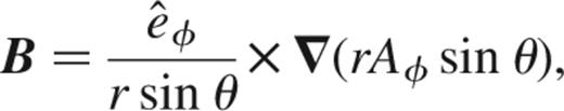
so that the quantity rA sin θ labels the magnetic field lines.
Rewriting equation (1), we find that the time evolution of A is given by
We now separate A into radial and angular parts,
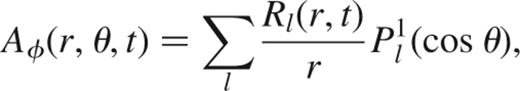
where  is the associated Legendre function of order one. The magnetic field components are
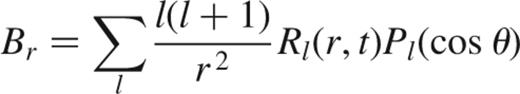
and
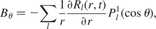
where Pl is the Legendre polynomial. We use spherically symmetric white dwarf models1 in which the diffusivity depends on the radius r only, and not on the latitude θ. In this case, substituting equation (6) into equation (5) gives
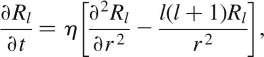
which is a diffusion equation for the radial function Rl.
Neglecting mass and density changes because of accretion, the conductivity of a liquid white dwarf is independent of time, and depends only on position, η(r). In this case, we follow WVS, and look for a solution that decays exponentially with decay time τln,
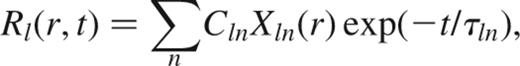
where Cln is a constant giving the contribution of mode n, and the differential equation
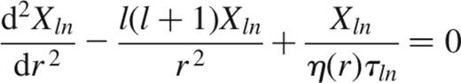
determines the eigenfunction Xln(r).
We adopt the following boundary conditions (see the discussion in Section 5.6 of Mestel 1999). Inspection of equation (11) shows that a finite solution at the centre of the star must have Xln∝rl+1, giving
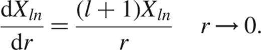
Outside the star, where the current J∝∇×B=0, we choose the solution that remains finite for large r, Rln∝r-l. Thus, we take
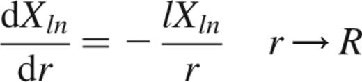
at the surface.
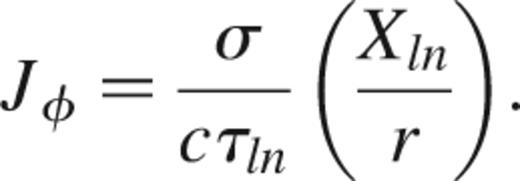
Solution of equation (11) requires knowing the conductivity as a function of radius. This is shown in the top panel of Fig. 2 for a 0.6-M⊙ white dwarf, normalized to the central value, σc=9.6×10²⁰ s-1. The resulting n=1 and 2 dipole (l=1) decay modes Xln are shown as solid lines in the middle panel of Fig. 2. The lower panel shows the current density J=(c/4π)∇×B. Using equations (5), (6) and (10), this may be written in terms of Xln as J=Je^, where
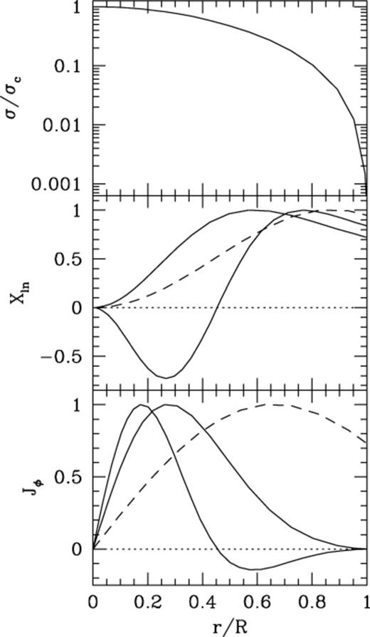
Ohmic decay modes for a 0.6-M⊙ white dwarf. (i) In the upper panel, we show the conductivity as a function of radius. The central value of conductivity in this model is ≈1021 s−1, dropping to close to the Spitzer value ≈5×10¹⁷ s−1 (equation 19) at the outer boundary. (ii) In the middle panel we show the n=1 and 2 dipole (l=1) decay modes. We normalize each eigenfunction so that its maximum value is unity. The nth mode has (n-1) nodes. The dashed curve shows the n=1 mode for constant conductivity with radius. (iii) The lower panel shows the distribution of current density for the eigenmodes shown in the middle panel.
Note that the nth mode has n-1 nodes, with the current reversing direction at a node.
Table 1 gives the decay time for modes with l=1,2 and 3, and n=1,2 and 3 for 0.6 and 1.0-M⊙ white dwarfs. For both white dwarf masses, we find that the lowest-order decay mode (l=1 and n=1) has a decay time τ11≈tohm/40, roughly a factor of 4 smaller than the analytic result for η independent of radius (in which case τ11=tohm/π2, see WVS equation 10).
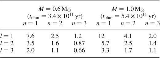
Ohmic decay times (τln in units of 109 yr).
The decay times in Table 1 agree well with the calculations of WVS for liquid white dwarfs (cf. their fig. 2). However, we do not agree with the later calculations of MVW, who report decay times that are an order of magnitude smaller, (3–10)×108 yr, for liquid white dwarfs (see their Section 3.3), despite using the same conductive opacities for the liquid interior as WVS (see their Section 2.3). The origin of this difference is not clear. The central conductivity quoted by MVW for a 0.6-M⊙ white dwarf (≈2×10²¹ s−1) agrees to within a factor of 2 with the value in our models and those of WVS. In addition, changing the conductivity profile seems unlikely to give an order of magnitude change in the decay time. The difference may be caused by an incorrect normalization used by MVW (H. van Horn, private communication).
To test the influence of the conductivity profile, we compared our eigenfunctions with those of WVS and MVW (fig. 3, left-hand panel, of WVS; fig. 1, top panel of MVW). The agreement is good for times ≳109 yr, but differs for earlier times, for which the eigenfunctions of the WVS and MVW peak at larger radius (r/R≈0.8 rather than r/R≈0.6). We have been unable to identify the reason for this difference. The peak at larger radius probably reflects a shallower conductivity profile. For example, in the extreme case of constant conductivity with radius, the currents are less centrally concentrated than in realistic models. The reason for this is that the currents flow in the regions of high conductivity; this region is more extended in the constant-conductivity model. The dashed lines in the middle and lower panels of Fig. 2 show the n=1, l=1 eigenmode for constant conductivity [in this case X11∝rj1(r), where j1 is the spherical Bessel function of degree one, see WVS]. As noted above, the lowest-order decay time for constant conductivity is a factor ≈4 longer than the realistic white dwarf models.
In summary, we find that the ohmic decay time lies in the range ≈(8–12)×109 yr for a dipole field, and ≈(4–6)×109 yr for a quadrupole field, depending only slightly on the white dwarf mass.
3 Accretion versus diffusion times in the envelope
The long time-scale for ohmic decay raises the question of the effect of the accretion flow on the magnetic field structure. The decay time-scale of ≈1010 yr is the time to accrete the whole star at 10−10 M⊙ yr−1. For more rapid accretion than this, one might expect the magnetic field structure to be altered significantly as the magnetic field is advected by the accretion flow.
In fact, the evolution of the magnetic field depends on the local accretion and diffusion time-scales at different depths in the white dwarf envelope. In this section, we compute these time-scales, before moving on to simple models of the global field structure in Section 4.
3.1 Analytic estimates
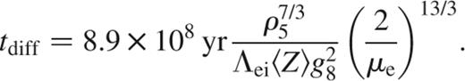
We consider the outer layers of the star, where the gravity g=GM/R2 is constant. We define the column depth y=-∫ρ dz=ΔM/4πR2, where ΔM is the mass above the column depth y. Hydrostatic balance dP/dz=-ρg becomes dP/dy=g, giving P=gy. The time to accrete the matter above a given column depth is taccr=y/m·, where m·=M·/4πR2 is the local accretion rate per unit area. We compare this with the ohmic diffusion time across a scaleheight, tdiff=4πσH2/c2.
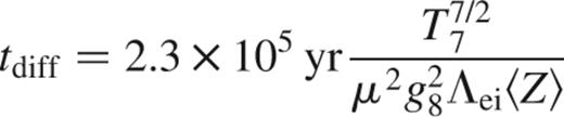
When the electrons are degenerate, the conductivity is given by equation (3). In the outer layers, the electrons are non-relativistic, so that  . The pressure scaleheight is H=P/ρg=6.8×107 cm
 , giving
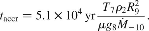
To evaluate the accretion time-scale, we write the local accretion rate m·=m·-310-3 g cm-2 s-1 in terms of the global rate M·=M·-1010-10 M⊙ yr-1, as m·=M·/4πR2, giving
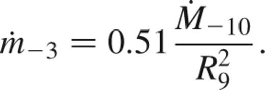
If accretion is not occurring over the whole surface of the white dwarf (for example, magnetically controlled accretion on to the polar caps), the relevant quantity is the local accretion rate; we work in terms of the global rate only for convenience. We find
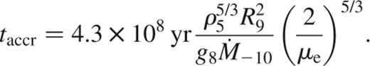
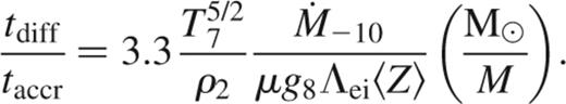
The ratio of tdiff to taccr depends on the quantity gR2, which we rewrite in terms of the mass of the star,  . This gives
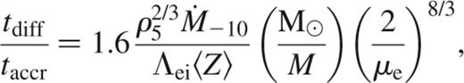
which depends only weakly on depth.
Equation (18) shows that tdiff≈taccr for accretion rates of the order of 10-10 M⊙ yr-1. This is roughly the same critical accretion rate as found for the degenerate ocean of an accreting neutron star in CZB (cf. equation 29 of that paper). The reason is that tdiff/taccr∝1/gR2, so that it depends only on the mass M and not separately on the gravity and radius.
At densities ≲103 g cm−3, the electrons become non-degenerate, in which case the conductivity is given by Spitzer's formula (Spitzer 1962)
where the temperature T=T7107 K. For an ideal gas, the pressure scaleheight is H=P/ρg=kBT/μmpg, where μ is the mean molecular weight, giving H=8.3×10⁶ cmT7/μg8. The ohmic time is
and the accretion time is
The ratio of the two is
We have inserted typical values for temperature and density, although the exact value of this ratio depends on the T–ρ relation in the atmosphere. For a constant-flux atmosphere with free–free opacity, T∝ρ4/13, giving tdiff/taccr∝ρ-3/13, which is again weakly dependent on density.
3.2 Detailed models
We calculate models of the atmosphere by integrating the heat flux equation
and the entropy equation
where κ is the opacity, cP is the specific heat at constant pressure and the adiabatic index is ∇ad=(d ln T/d ln P)ad. The terms on the right-hand side of equation (24) represent the effects of compressional heating (Nomoto 1982; Townsley & Bildsten 2001, 2002).
We integrate equations (23) and (24) from the top of the atmosphere to the base, iterating the choice of flux at the top until we match the correct flux from the core. We calculate the opacity, which includes contributions from free–free, electron scattering and conduction, as described by Schatz et al. (1999). Our calculation of electrical conductivity, which reduces to equation (3) for degenerate electrons, and equation (19) for non-degenerate electrons, is described in the Appendix.
As an illustrative model of the outer layers of an accreting white dwarf, we take a layer of solar abundance material of mass 10−5 M⊙, a pure helium layer of mass 10−2 M⊙ and a white dwarf mass of 0.6 M⊙, with an equal mixture by mass of carbon and oxygen in the core. We choose a luminosity from the core of 10−3 L⊙. We show the resulting temperature profiles for M·=10-10 and 10-9 M⊙ yr-1 in Fig. 3. For M·=10-10 M⊙ yr-1, we find a core temperature of 9.4×10⁶ K, luminosity of 4.7×10⁻³ L⊙ and effective temperature of 13 600 K. For M·=10-9 M⊙ yr-1, we find a core temperature 2.0×10⁷ K, luminosity of 6.2×10⁻² L⊙ and effective temperature of 25 900 K. These values are in reasonable agreement with the detailed models of compressional heating presented recently by Townsley & Bildsten (2001, 2002). A simple estimate of the compressional heating luminosity is to write
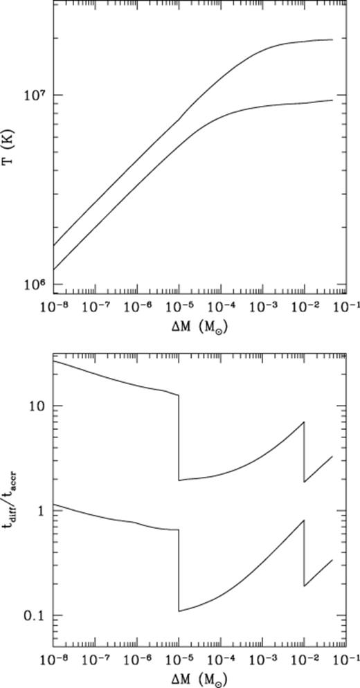
(i) Temperature profiles in the white dwarf envelope for M·=10-10 (lower curve) and 10−9 M⊙ yr−1 (upper curve), for a 0.6-M⊙ white dwarf. (ii) Ratio of ohmic time to accretion time in the envelope for M·=10-10 (lower curve) and 10−9 M⊙ yr−1 (upper curve). The composition is solar for ΔM<10-5 M⊙, pure He for 10-5 M⊙<ΔM<10-2 M⊙, and C/O for ΔM>10-2 M⊙.

where we use the heat capacity of an ideal gas cP=5kB/2μmp, and take μ≈1 as a mean value in the envelope. This estimate agrees well with our numerical results.
The ratio tdiff/taccr is shown in Fig. 3, and the ohmic time and accretion time individually in Fig. 4. Our numerical results agree well with the analytic estimates in Section 3.1. In the degenerate layers (ΔM≳10-5), tdiff/taccr increases with depth (equation 18). The jumps in tdiff/taccr at ΔM=10-5 M⊙ and ΔM=10-2 M⊙ result from the changes in composition from solar to pure He and from pure He to C/O (equations 18 and 22 give tdiff/taccr∝1/〈Z〉). At low densities, tdiff/taccr decreases with depth, as expected from equation (22).

Ohmic diffusion time (solid lines) and accretion time (dotted lines) in the white dwarf envelope for the models of Fig. 3(M·=10-10 and 10-9 M⊙ yr-1). The accretion time (dotted lines) is labelled with the appropriate accretion rate (the accretion time is smaller for a higher accretion rate). The diffusion time (solid lines) is independent of the accretion rate in the degenerate layers (the conductivity depends only on density); but is longer for higher accretion rates in the non-degenerate layers (the conductivity increases with temperature).
The condition tdiff=taccr defines a critical accretion rate M·c. Inspection of Fig. 3 shows that for the accreted envelope (ΔM<10-5 M⊙),M·c≈10-10 M⊙ yr-1, and for the He layer and the C/O core, an average value is M·c≈5×10⁻¹⁰ M⊙ yr-1. This agrees well with our analytic estimates (cf. equations 18 and 22 when tdiff/taccr=1).
4 global models of accretion and diffusion
In this section, we follow the effects of advection and diffusion in a simple model of the global magnetic field structure. We show that the evolution is very different depending on whether M· is less than or greater than the critical rate M·c≈(1–5)×10-10 M⊙ yr-1 found in Section 3.
4.1 A simple model of the global field evolution
We make the following simplifying assumptions: (i) we consider an axisymmetric, poloidal magnetic field, (ii) we assume spherical accretion; and (iii) we take the accreted matter to have the same composition as the core (equal amounts by mass of C and O). Under spherical accretion, each spherical harmonic component l evolves independently, so that an initially dipolar field remains dipolar as accretion proceeds. In reality, the accreted matter is channelled on to the polar caps in magnetic systems, subsequently spreading over the surface of the star. We do not attempt to model this process here, meaning that we must pay careful attention to our choice of surface boundary condition. We discuss this issue below, but first outline the equation describing the evolution of the magnetic field, and how we solve it.
The induction equation with advection included is
or, in terms of the vector potential A,

As previously, we consider an axisymmetric field, so that A=A(r,θ)e^. In the absence of diffusion, equation (27) gives
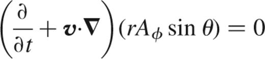
(WVS, Choudhuri & Konar 2002). The quantity rA sin θ (which labels the magnetic field lines, see Section 2.2) is advected by the poloidal velocity field.
As before, we separate A into radial and angular parts according to equation (6). We take the velocity field to be purely radial, v=vr(r,θ)e^r. Equation (27) then gives
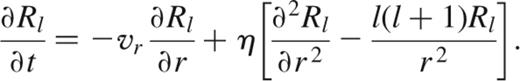
This equation governs the evolution of Rl(r, t) under the joint action of accretion and diffusion.
We evolve equation (29) numerically.2 At each time-step, we include advection by making a new white dwarf model (as described in Section 2.1) with a slightly larger mass, but keep Rl fixed for a given fluid element. We then apply an implicit Crank–Nicholson scheme for the diffusion term (e.g. Press et al. 1992). With accretion switched off, our code accurately follows the predicted decay of the eigenmodes found in Section 2.
We adopt two different boundary conditions at the surface. The first is the ‘vacuum’ boundary condition given by equation (13). The second boundary condition is a ‘screened’ boundary condition Rl=0 at the surface. In the advection step, the boundary condition determines the values of Rl assigned to the newly accreted matter. As described above, we take the composition of the accreted material to be equal mass fractions of C and O. At the centre of the star, where vr vanishes, we apply equation (12).
The ‘vacuum’ boundary condition implies J=0 outside the star, as in Section 2, and that each shell of matter is accreted with the vacuum field at the surface. This boundary condition was adopted by Choudhuri & Konar (2002) in their recent study of accreting neutron stars [these authors solved equation (27) with a prescribed two-dimensional velocity field]. In our one-dimensional model, we envisage this boundary condition as approximating the case where the accreted material is able to spread away from the polar cap without significantly distorting the field structure. This is similar to the approach of Choudhuri & Konar (2002), who put in an outwards radial velocity in the outer layers to simulate the effects of buoyancy instabilities. They found that the evolution of the field was then determined by advection in the interior. The ‘screened’ boundary condition Rl=0 assumes screening currents at the surface, similar in spirit to the plane-parallel models of CZB for accreting neutron stars, and to the idea that the magnetic field may be completely buried by accretion.
These two different boundary conditions illustrate the range of behaviour that might be expected given a more complex flow geometry and better treatment of the outer layers, including effects such as buoyancy or interchange instabilities. However, note that the solution for the interior is insensitive to the choice of surface boundary condition. In the next section, we present our numerical results. We show that the evolution of the field depends upon whether the accretion rate is above or below the critical rate M·c.
4.2 Results
Fig. 5 shows the time evolution of a dipole field during accretion of 0.1 M⊙ on to a 0.6-M⊙ white dwarf at two different accretion rates. We take a ‘vacuum’ boundary condition, and the initial profile of R1(r) to be the lowest-order dipole decay mode. We show the time evolution of R1, Br(∝R1/r2, equation 7), and B[∝(1/r)(dR1/dr), equation 8] at equal steps in central density. We normalize R1 so that the initial profile has a maximum value R1=1, and normalize Br and B so that the initial central value is unity. The initial central density is ≈3×10⁶ g cm−3, increasing to ≈6×10⁶ g cm−3. The left-hand panel is for M·=10-10 M⊙ yr-1, in which case the accretion lasts for 109 yr, and the right-hand panel is for M·=10-9 M⊙ yr-1, in which case the accretion lasts for 108 yr.
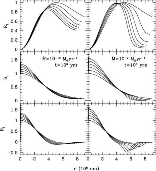
Time evolution of the magnetic field during accretion of 0.1 M⊙ on to a 0.6-M⊙ white dwarf. We assume ‘vacuum’ boundary conditions (see the discussion in Section 4.1). The left-hand panel shows M·=10-10 M⊙ yr-1, for which the accretion takes 109 yr; the right-hand panel shows M·=10-9 M⊙ yr-1, for which the time elapsed is 108 yr. The curves are spaced by equal increments in central density, which increases from ≈3×10⁶ to ≈6×10⁶ g cm−3. We normalize R1 to have a maximum value of R1=1 initially, and normalize Br and B to have a central value of unity initially.
At M·=10-10 M⊙ yr-1 (left-hand panel of Fig. 5), the magnetic field has time to diffuse into the newly accreted material. The overall decrease in R1 is caused by ohmic decay during the 109 yr of accretion (the lowest-order decay time of the initial model is τ11=7.6×10⁹ yr). At M·=10-9 M⊙ yr-1 (right-hand panel of Fig. 5), the accreted material is added too quickly for significant diffusion, so that the surface value of R1 drops as accretion proceeds. The central values of Br and B increase by a factor of ≈1.6. This can be understood in terms of the combination of flux conservation, which gives r2B=constant, and mass conservation, which gives r3ρ=constant. Eliminating r, we find B∝ρ2/3, giving an increase in B of 1.6 when ρ increases by a factor of 2. (In the thin layer considered by CZB, the compression was one-dimensional, giving B∝ρ in that case; see their equation 13.)
Fig. 6 shows the final magnetic profiles for accretion at several different rates. We show the profiles for vacuum boundary conditions (left-hand panel) and screened boundary conditions (right-hand panel). The initial profile in each case is shown by the dashed line, and is the lowest-order decay mode of the initial model (subject to the respective surface boundary condition). We show accretion rates of M·=10-11, 10−10, 10−9 and 10−8 M⊙ yr−1. At the lowest accretion rates, 10−11 and 10-10 M⊙ yr-1 (dotted lines), the magnetic field is able to diffuse into the newly accreted layers. The decrease in R1 is caused by ohmic decay over the long time-scale of accretion. For accretion rates 10−9 and 10-8 M⊙ yr-1 (solid lines), the accreted layers do not have time to become significantly magnetized. At M·=10-8 M⊙ yr-1, the final profile is almost exactly that given by conserving R1 in each fluid element as accretion proceeds.
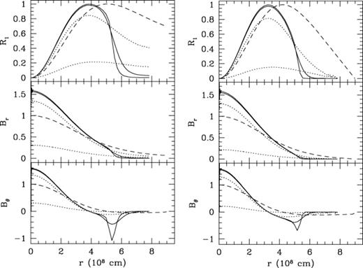
The profiles of R1, Br and B after the accretion of 0.1 M⊙ on to a 0.6-M⊙ white dwarf at different rates. We show results for vacuum boundary conditions (left-hand panel) and screening boundary conditions (right-hand panel). The dashed line in each panel shows the initial state. The solid lines show accretion rates of 10−8 and 10-9 M⊙ yr-1, for which mass is accreted too rapidly to become significantly magnetized. The dotted lines show accretion rates of 10−10 and 10-11 M⊙ yr-1, for which ohmic diffusion has time to magnetize the accreted material. Significant ohmic decay of the field occurs at these low rates, because the accretion takes a long time.
In Figs 7 and 8, we show the magnetic field lines for the profiles in Fig. 6. We show field lines with the same values of rA sin θ in each panel. The M·=10-11 M⊙ yr-1 model has only a small number of field lines because of the significant ohmic decay that occurs as accretion proceeds. At 10-9 M⊙ yr-1, most of the field lines shown in the initial model have been pushed into the interior by the accretion flow.
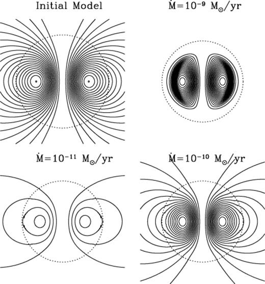
Magnetic field lines for the models shown in the left-hand panel of Fig. 6. We show the initial field structure in the top left-hand panel, and the final structure for (clockwise from the top right) M·=10-9, 10−10 and 10-11 M⊙ yr-1. The dotted line indicates the stellar surface (note the larger radius of the less massive initial model). We show field lines with the same value of flux in each panel. The dramatic ohmic decay at the lowest accretion rate appears as the reduction in the number of field lines.
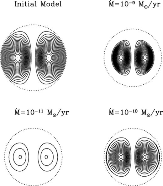
Fig. 9 shows R1, Br and B at the surface as a function of mass accreted for a vacuum boundary condition. As we discussed in Section 4.1, the quantitative decrease in the surface field depends on the chosen surface boundary condition. However, Fig. 9 shows the qualitative effect of accretion at different rates. From top to bottom, the accretion rates are M·=10-10, 10−11 and 10-9 M⊙ yr-1. At M·=10-10 M⊙ yr-1, the surface field changes only slightly as the newly accreted material is able to become magnetized by diffusion. For M·=10-11 M⊙ yr-1, the surface field decreases owing to ohmic decay (in this case the accretion takes 1010 yr, which is comparable to the decay time). For M·=10-9 M⊙ yr-1, the change is caused directly by accretion.
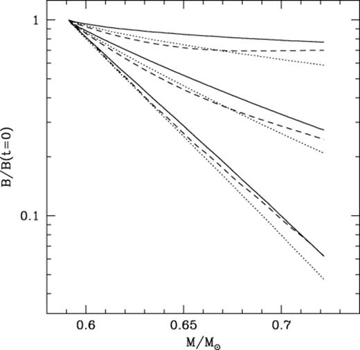
For the vacuum boundary condition solutions, we show surface values of R1 (dotted line), Br (solid line) and B (dashed line) relative to their initial values as a function of white dwarf mass for (top to bottom) M·=10-10, 10−11 and 10-9 M⊙ yr-1.
5 Implications for observed systems
In the previous sections, we have shown that, under the assumption that the white dwarf retains the mass it accretes, the surface magnetic field may be reduced significantly for accretion rates greater than the critical value M·c≈(1–5)×10-10 M⊙ yr-1. We now conclude by discussing the implications of our results for observed systems. We show that there are several interesting consequences of abandoning the assumption that the magnetic fields of accreting white dwarfs do not change with time.
5.1 An evolutionary connection between AM Hers and intermediate polars?
Accreting white dwarfs fall into two classes. Those in AM Her systems rotate synchronously with the binary orbital period, and have fields 107–3×10⁸ G (WF). Intermediate polars (see the review by Patterson 1994), in which the white dwarf rotates asynchronously, are believed to contain white dwarfs with fields ∼105–107 G, although most have not been measured directly (the lower limit here is the field strength needed to disrupt the accretion flow before it hits the white dwarf surface). The asynchronous rotation of the white dwarfs in IPs lead to early suggestions that the white dwarf magnetic fields are lower than in AM Hers [for example, Lamb & Patterson (1983) estimated B∼106 G]. In addition, whereas strong optical polarization is seen in AM Hers, little or no polarization is seen in IPs, also suggesting weaker magnetic fields. Recently, the lack of Zeeman splitting in spectroscopic observations of the white dwarf in V709 Cas (Bonnet-Bidaud et al. 2001) has constrained the magnetic field to be <107 G.
The two classes show an interesting difference in accretion rates. AM Her systems accrete at low rates, M·≈5×10-11 M⊙ yr-1 (Chanmugam, Ray & Singh 1991, Warner 1995), whereas the IPs accrete rapidly, Warner (1995) estimates M·≈(0.2–4)×10-9 M⊙ yr-1 from X-ray fluxes of ten systems. Wickramasinghe & Wu (1994) propose that the low accretion rate of AM Hers is a direct consequence of the strong magnetic field of the white dwarf, which inhibits magnetic braking by reducing the number of open field lines along which the magnetized wind from the secondary may flow (for example, see Li, Wickramasinghe & Wu 1995).
Fig. 10 shows the orbital period distributions of known AM Hers and IPs. Most AM Her systems have Porb≲3 h, whereas most IPs have Porb≈3–6 h. This difference has led many to suggest an evolutionary link between the two classes, namely that the asynchronous IPs are the progenitors of the synchronous AM Her systems. For a magnetic field B∼107 G, the magnetospheric radius equals the orbital separation at Porb≈4 h, suggesting a natural dividing line between synchronous and asynchronous systems (Chanmugam & Ray 1984, King, Frank & Ritter 1985, Hameury et al. 1987). However, demonstrating an evolutionary connection is difficult if the white dwarf magnetic field is constant with time (e.g. Wu & Wickramasinghe 1993). It requires that either (i) the IPs and AM Hers have similar magnetic field strengths, but the optical polarization is somehow suppressed in asynchronous rotators, or (ii) the IPs have weaker fields than the AM Her systems, implying a yet to be detected population of asynchronous AM Her progenitors (King & Lasota 1991).
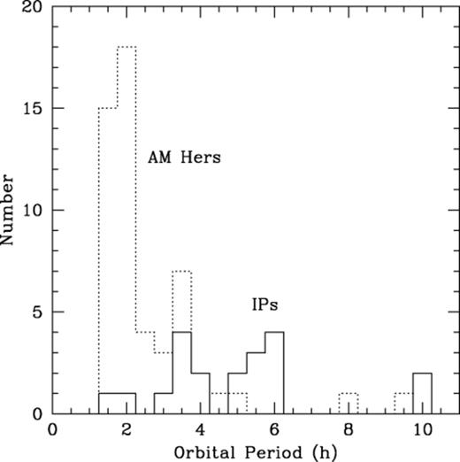
The orbital periods of AM Her systems and intermediate polars. We show orbital periods for 53 AM Her systems from Wickramasinghe & Ferrario (2000), and for 20 intermediate polars from the catalogue of Ritter & Kolb (1998). We exclude the intermediate polar GK Per, which has Porb=2 d and an evolved companion.
It is striking that the mean accretion rate of the IPs is >M·c, whereas the AM Her systems accrete at rates <M·c. Thus, given our results, a natural suggestion is that the magnetic fields of the intermediate polars are low because of the direct effect of the accretion flow. If so, it is possible for an intermediate polar to evolve into an AM Her system if the mass transfer rate drops from >M·c to <M·c at an orbital period ≈(3–4) h (between the observed AM Her and intermediate polar populations).
The reason for such a change in accretion rate is not clear, but is reminiscent of the need for a rapid drop in mass transfer rate to explain the period gap (Porb≈2–3 h) in non-magnetic cataclysmic variables (CVs). Whether or not the magnetic CVs exhibit a period gap is unclear, there are certainly a higher fraction of magnetic systems in the gap than for non-magnetic systems (King 1994, Kolb 1995, Wheatley 1995). It is, however, possible that a similar mechanism is operating in both cases, perhaps disrupted magnetic braking, as preferred for non-magnetic systems (Rappaport, Verbunt & Joss 1983, Howell, Nelson & Rappaport 2001).
There is an alternative scenario along the same lines as that of Wickramasinghe & Wu (1994). The ROSAT detection of IPs with soft X-ray spectra similar to the weaker field AM Hers (Haberl & Motch 1995) has led to suggestions of two populations of IPs. A possibility is that those IPs with fields close to 107 G come into synchronous rotation at Porb≈4 h, which causes a drop in M· as suggested by Wickramasinghe & Wu (1994), allowing the field to subsequently grow to values ∼108 G typical of AM Hers. A problem with this picture is what happens to the weaker field IPs (i.e. those with traditional hard X-ray spectra), since very few of them are seen at short orbital periods.
The time-scale for re-emergence of the field is set by the ohmic diffusion time at the base of the accreted layer. Fig. 4 and equation (16) show that this is ≈3×10⁸ yr(ΔM/0.1 M⊙)7/5, where ΔM is the accreted mass. This is similar to the time for a non-magnetic CV to cross the period gap (Howell et al. 2001). Thus if the drop in mass accretion rate causes the secondary to lose contact with the Roche lobe, there may be time for the field to re-emerge before contact is resumed. The impact of any gap on the observed orbital period distribution depends on how strongly the transition orbital period depends on the mass transfer rate and the magnetic field. With or without a period gap, the lack of known synchronous low-field systems could constrain the time-scale for re-emergence and therefore the accreted mass.3
A detailed test of either scenario requires a comparison of evolutionary studies and the observed populations of IPs and AM Hers. We note that, whereas there is a clear difference in orbital periods and magnetic field strengths between AM Hers and IPs as classes of objects, no correlation is observed between the magnetic field strength and the orbital period amongst AM Her systems only (WF).
5.2 Where are the 109-G accreting white dwarfs?
The highest measured magnetic field in an accreting system is 2.3×10⁸ G for AR Uma, whereas the highest observed fields in isolated WDs are close to 109 G. Whether or not this difference is significant remains to be seen. For example, WF argue that selection effects hide the very high-field accreting WDs. There have been suggestions as to why the observed upper limit might differ. Wickramasinghe & Wu (1994) argue that because the high-field systems come into synchronization at wider separation, magnetic braking is suppressed earlier, and they do not have time to evolve via gravitational radiation into contact (thus they predict a population of high-field, detached binaries).
We would like to point out that some difference would be expected simply because of the different ohmic decay properties of the two populations. The liquid accreting white dwarfs decay at a faster rate than the isolated white dwarfs, which form a solid core after ∼109 yr of cooling, effectively switching off ohmic decay. To find the maximum difference between the two populations, we assume that the isolated white dwarfs undergo no magnetic field decay. The contrast in field strengths is then exp(t/τ), where τ is the decay time for the accreting population. For τ=1010 yr, this gives a factor of 2 after t=7×10⁹ yr, or a factor of 3 after t=11×109 yr. This effect alone may not explain the observed factor of ≈3, but should be taken into account when comparing the maximum field strengths of the two populations.
5.3 Type Ia progenitor systems
Currently favoured models for type Ia supernovae progenitors are rapidly accreting (M·≳10-7 M⊙ yr-1) massive white dwarfs, which are able to burn the accreted hydrogen and helium steadily and grow to near-Chandrasekhar mass. Examples are the white dwarfs in supersoft X-ray sources and symbiotic binaries. If accretion is acting to suppress the surface magnetic field in these sources as we propose for intermediate polars, we would not expect to find strongly magnetic white dwarfs in these systems. There is little information concerning the incidence of magnetism in these rapidly accreting systems. In a survey of 35 symbiotics, Sokoloski & Bildsten (1999) (see also Sokoloski, Bildsten & Ho 2001) discovered a magnetic WD in the symbiotic binary Z And rotating with a 28-min spin period. If the white dwarf is in spin equilibrium with an accretion disc at the magnetospheric radius, the implied magnetic field strength is 6×10⁶ G, typical of an intermediate polar. XMM observations of M31 revealed a supersoft X-ray source with 865 s pulsations, interpreted as being a result of the spin of a magnetized white dwarf (Osborne et al. 2001). A similar estimate for the magnetic field gives ≈107 G (King, Osborne & Schenker 2002). It remains to be seen how common systems such as these are amongst rapidly accreting sources.
As the central density increases because of accretion, the internal field is amplified by compression (B∝ρ2/3; see Section 4.2). This amplification is shown in Fig. 5 for accretion on to a 0.6-M⊙ white dwarf, and would be even greater for a massive white dwarf. The density increases especially quickly as you approach the Chandrasekhar mass and the electrons become more relativistic, as pointed out by work on compressional heating (Nomoto 1982; Townsley & Bildsten 2001, 2002). An important problem is to understand the role played by such an amplified magnetic field in the approach to and evolution after ignition of a type Ia supernova. For example, Ghezzi et al. (2001), recently pointed out that a large-scale magnetic field of 108–109 G can generate asymmetries in the thermonuclear flame front that engulfs the white dwarf during the supernova. Our results show that the prior evolution of the field during accretion should be taken into account.
5.4 Complexity as a result of accretion
Both isolated and accreting white dwarfs often show a complex magnetic field geometry, requiring a significant quadrupole component or an offset dipole (WF). In Section 2, we found decay times of (4–6)×109 yr for the l=2 decay mode of liquid white dwarfs. Thus one possibility is that the quadrupole field is a fossil field, requiring that the dipole and quadrupole fields had comparable magnitudes initially.
In isolated systems, the liquid decay time is relevant only for the first ∼109 yr, after which the formation of a solid core increases the ohmic time. Muslimov et al. (1995) studied the Hall effect in isolated white dwarfs as a possible mechanism for generating field complexity as the white dwarf cools. However, the Hall effect is not expected to play a significant role for a liquid interior (Muslimov et al. 1995).
Another possibility is that the accretion flow leads directly to the complexity of the field. The spreading of material away from the polar cap (which we have not included in our models in this paper) could induce higher-order components of the surface field. An interesting observation is that the magnetic pole undergoing most accretion in AM Her systems is the pole with the weaker magnetic field in all cases with magnetic field measurements for both poles (WF). Wickramasinghe & Wu (1991) suggest that this is a result of the role of the quadrupole component during synchronization. An alternative suggested by our results is that after synchronization occurs, the pole pointing towards the companion undergoes more rapid accretion, which reduces the field strength at that pole, giving rise to the observed asymmetry. Even though the global rate for AM Hers is <M·c, the local accretion rate in the layers for which the accreted material is still confined to the polar cap will be greater than the critical rate. Detailed models of the spreading of material away from the polar cap are required to investigate this further.
6 Conclusions
We have studied the evolution of the magnetic field in an accreting white dwarf. Previous studies of ohmic decay in isolated white dwarfs showed that the ohmic decay time is always longer than the cooling time because the white dwarf develops a solid core. In Section 2, we calculated the ohmic decay times for the lowest-order modes of accreting white dwarfs, which have a liquid interior because of compressional heating by accretion. We found that the lowest-order ohmic decay time is (8–12)×109 yr for a dipole field, and (4–6)×109 yr for a quadrupole field (see Table 1), in good agreement with the earlier calculations of WVS. The difference in ohmic decay times between isolated and accreting white dwarfs should be taken into account when comparing the maximum field strengths of the two populations. In addition, the decay time-scale for the quadrupole is long enough that observed quadrupole components (see WF for a summary of the observations) in both accreting and isolated white dwarfs may be fossil if the quadrupole is initially of similar strength to the dipole component.
In Section 3, we compared the time-scale for ohmic decay with accretion, and showed that accretion occurs more rapidly than ohmic diffusion for accretion rates greater than the critical rate M·c≈(1–5)×10-10 M⊙ yr-1. In Section 4, we calculated the time evolution of the magnetic field as a function of the accretion rate, assuming that the white dwarf mass increases with time. For a simplified field and accretion geometry (an axisymmetric poloidal magnetic field and spherical accretion), we found that accretion at rates M·>M·c leads to a reduction in the field strength at the surface, as the field is advected into the interior by the accretion flow.
The main conclusion of this paper is that, because of the direct action of accretion, significant changes in the surface magnetic field of an accreting white dwarf could occur during its accretion lifetime. In Section 5, we showed that accretion-induced magnetic field evolution may explain several features of the observed systems. Most striking is that the strongly magnetic (B∼107–3×10⁸ G) AM Her systems have a mean accretion rate ≈5×10⁻¹¹ M⊙ yr−1<M·c, whereas the weakly magnetic (B∼105–107 G) IPs accrete at rates ∼10−9 M⊙ yr−1>M·c. This raises the possibility that the white dwarfs in IPs have subsurface fields as strong as those in AM Hers. If so, this allows for an evolutionary connection between the long orbital period (Porb≈3–6 h) IPs and short orbital period AM Hers (Porb≲3 h), requiring that evolution in orbital period somehow causes a drop in accretion rate (for example, by disrupted magnetic braking as postulated for non-magnetic CVs; see Section 5.1 for a further discussion). The magnetic field would then re-emerge on a time-scale set by ohmic diffusion, ≈3×10⁸ yr(ΔM/0.1 M⊙)7/5, where ΔM is the accreted mass. Evolutionary calculations are necessary to compare this scenario with the properties of observed systems. We did not consider non-magnetic accreting systems in Section 5; however, it is possible that many non-magnetic white dwarfs (meaning B≲105 G so that the accretion flow is not disrupted) have submerged magnetic fields if they are accreting at rates >M·c.
The models presented in this paper are simplified, and many outstanding theoretical questions remain. The major uncertainty in the evolution of accreting white dwarfs is whether the white dwarf mass increases or decreases with time. Even if the mass is increasing with time as we have assumed here, classical nova explosions eject some mass from the system; the effective mass accretion rate is therefore less than the mass transfer rate from the secondary by some factor, introducing an extra uncertainty. If classical novae eject more mass than is accreted prior to thermal runaway, excavation of the white dwarf core leads to a decreasing mass with time. This raises the possibility that the surface magnetic field could grow with time if the underlying magnetic field is exposed as the mass decreases. This was originally suggested as a source for the magnetic field of DQ Her by Lamb (1974). Interestingly, this alternative is also consistent with an evolutionary link between AM Hers and intermediate polars, since the magnetic field would increase as the orbital period decreases and successive nova explosions occur. The evolution of the magnetic field under the action of mass loss is left to a future study. The result is presumably somewhat dependent on the initial choice for the current distribution, and differences in the thermal evolution will have to be taken into account.
It is important to understand the spreading of matter away from the polar cap. This topic has received little attention, and is not well understood. Studies of the polar cap of accreting neutron stars (Hameury et al. 1983, Brown & Bildsten 1998, Litwin, Brown & Rosner 2001) and white dwarfs (Livio 1983, Hameury & Lasota 1985) suggest that spreading occurs once the sideways force caused by the hydrostatic overpressure overcomes the confining magnetic tension, or sooner if instabilities play a role (Litwin et al. 2001). Understanding the spreading process, and its effect on the magnetic field geometry in the outermost layers of the star is directly relevant for interpreting observations of polar cap fields of AM Hers. A related issue that remains to be explored is the stability of the magnetic field configurations found in Section 4. For example, stability considerations demand a toroidal field component that is not included in our simple models (see the discussion in Mestel 1999).
Finally, we have not discussed the effect of white dwarf rotation. As mentioned in the introduction, King (1985), applying the results of Moss (1979) to accreting white dwarfs, suggested that meridional currents could be responsible for the submergence of magnetic flux in the outer layers of rotating magnetic white dwarfs. The aim was to explain the narrow range of field strengths in AM Hers. The effect of meridional flows in accreting white dwarfs deserves further investigation.
Acknowledgments
We thank Dayal Wickramasinghe for conversations concerning observations of magnetic white dwarfs, and Graham Wynn for emphasizing the lack of very strongly magnetic accreting white dwarfs. We are grateful to Ellen Zweibel for discussions concerning the appropriate surface boundary conditions in our global models, and to the referee Jean-Marie Hameury for carefully questioning our assumptions and conclusions. We thank Hugh van Horn and Alex Muslimov for communications regarding earlier work, Phil Arras and Chris Thompson for discussions concerning the Hall effect, and Dean Townsley and Lars Bildsten for discussions concerning their models of compressional heating. We acknowledge support from NASA through Hubble Fellowship grant HF-01138 awarded by the Space Telescope Science Institute, which is operated by the Association of Universities for Research in Astronomy, Inc., for NASA, under contract NAS 5-26555.
References
Appendix A: Electrical conductivity for arbitrary degeneracy
In the white dwarf envelope, the electrons go from being non-degenerate to degenerate. Hubbard & Lampe (1969) calculated the thermal conductivity for arbitrary degeneracy, presenting their results in tabulated form. Unfortunately, other calculations of conductivity that present their results in terms of fitting formulae, such as those of Yakovlev & Urpin (1980) and Itoh et al. (1983) are for degenerate electrons only (for thermal conductivity, this is the regime of interest, since radiative heat transport dominates at low densities). In their study of ohmic decay in cooling white dwarfs, WVS adopted an interpolation scheme between calculations in the degenerate and non-degenerate regimes. We have taken a different approach, which we describe below. After our calculations were completed, we learned of new conductivity calculations by Potekhin (1999) and Potekhin et al. (1999) that treat the regime of intermediate degeneracy. Comparing with these calculations, we find that our method agrees to within 20 per cent for degenerate electrons and to within a factor of 2 for non-degenerate electrons, which is adequate for our purposes.
For non-relativistic electrons, the density and electrical conductivity may be written
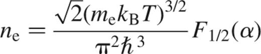
and
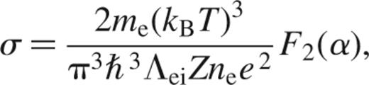
where α=-(EF-mec2)/kBT, and the Fermi integrals Fn(η) are given by
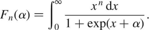
In equation (A2), we assume that the Coulomb logarithm Λei varies slowly enough with electron energy that it may be taken out of the integral. For degenerate electrons, α≪-1, equation (A2) reduces to the small-x (non-relativistic) limit of equation (3). For non-degenerate electrons, α≫1, equation (A2) reduces to equation (19) (Spitzer 1962).
Our approach in this paper is to evaluate σ using equation (A2), with Λei as a function of density, and with a correction for relativistic effects. We evaluate the Fermi integral F2(α) by direct numerical integration. The electron number density is used to determine α, by inverting equation (A1) using the fit of Antia (1993) to the inverse of F1/2.
We calculate the Coulomb logarithm as a function of density by interpolating between the non-degenerate result of Spitzer (1962) and the degenerate results of Yakovlev & Urpin (1980). We adopt the expression of Yakovlev & Urpin (1980) for the Coulomb logarithm, but rewrite it in terms of the electron momentum, choosing x in such a way that in the non-degenerate limit, we obtain Spitzer's formula. The Coulomb logarithm is  where
where  (YU). Here rmin and rmax are the limits of the integral over impact parameters. For temperatures greater than 4.2×10⁵ K (Spitzer 1962), rmin is set by the de Broglie wavelength of the electrons, we take rmin=ℏ/2pe. The cut-off rmax is set either by the Debye length, given by
  , or the interior spacing a=(3/4πni)1/3, whichever is larger. We obtain
where
[Hubbard & Lampe 1969;  , and where
  with
with  .
.
Finally, we include a correction for relativistic effects. Because we use equation (A1) to solve for α, we obtain the non-relativistic value for α in the degenerate limit, and equation (A2) reduces to the small-x limit of equation (3). To include relativistic effects, we divide equation (A2) by a factor of 1+x2, so that we recover equation (3) in full in the degenerate limit.
For the T=0 models of Sections 2 and 4, we write out  as a sum of logarithmic terms, but drop the term containing the temperature T, which contributes <10 per cent to the final value of Λei.
1 Except in the very outermost layers, it is always a good approximation that the hydrostatic pressure P is much larger than the magnetic pressure B2/8π.
2 This numerical approach is similar to that of WVS, who included the advection terms in their study of cooling white dwarfs. WVS found that the significant contraction that occurs in the pre-white dwarf stages of evolution increased the rate of ohmic decay, by taking the initial n=1 decay mode and generating higher-n components. This interesting effect is not significant during the accretion process, which involves much smaller changes in white dwarf radius.
3 We thank the referee, J.-M. Hameury, for raising this issue.
4 We thank Alexander Potekhin for bringing these results to our attention. Details of these calculations and computer codes to calculate conductivities can be found at http://www.ioffe.rssi.ru/astro/conduct/index.html.
Author notes
†Hubble Fellow.
