


Abstract
We present the results of multiple simulations of open clusters, modelling the dynamics of a population of brown dwarf members. We consider the effects of a large range of primordial binary populations, including the possibilities of having brown dwarf members contained within a binary system. We also examine the effects of various cluster diameters and masses. Our examination of a population of wide binary systems containing brown dwarfs, reveals evidence for exchange reactions whereby the brown dwarf is ejected from the system and replaced by a heavier main-sequence star. We find that there exists the possibility of hiding a large fraction of the brown dwarfs contained within the primordial binary population. We conclude that it is probable that the majority of brown dwarfs are contained within primordial binary systems which then hides a large proportion of them from detection.
1 Introduction
Brown dwarfs are essentially failed stars; they form within a stellar nebula just like any other star, but they fail to reach a mass that generates sufficiently high central temperatures and pressures to induce the process of hydrogen fusion. As a result of the lack of fusion, brown dwarfs are naturally very dark objects. The little light that they do put out is normally at the infrared end of the spectrum and is typically left-over energy from the accretion process.
The identification of brown dwarfs is a difficult process; their inherently faint magnitudes make them difficult to both locate and classify. Classification of brown dwarf status relies on the identification of spectral features from the object which couldn't have come from a low-mass star. The primary identifier of a brown dwarf is the presence of a lithium resonance doublet at 6708 Å. This feature up until recently proved very difficult to locate and the existence of isolated brown dwarfs was a subject of some controversy.
The first confirmed identification of a brown dwarf within the Pleiades cluster was by Basri, Marcey & Graham (1996) (Teide 1). They successfully identified, spectroscopically, the lithium feature in a brown dwarf candidate first discovered by Stauffer, Hamilton & Probst (1994). Since this first identification, the assignment of brown dwarf status has been given to many more candidate objects, particularly in the Pleiades cluster.
As a result of its low age and proximity, the Pleiades cluster is an excellent hunting ground for brown dwarfs. Many surveys have been made of this cluster; Hambly et al. (1999) performed a survey in the I and R bands and identified nine distinct single brown dwarf candidates. Further surveys have yielded more brown dwarf candidates within the cluster, notably a recent survey by Pinfield et al. (2000) has identified 30 possible brown dwarfs in a 6 deg2 survey of the cluster. Of particular interest is the work of Pinfield, Jameson & Hodgkin (1998). Their examination of the dynamics of the Pleiades cluster lead them to believe that there could be several thousand unseen brown dwarfs. If this is the case it is important to understand why so few brown dwarfs have been found within the central portions of the cluster which have been so well studied.
The discovery of Gliese 229B (a brown dwarf contained within a binary system) by Nakajima et al. (1995) (see also Golimowski et al. 1998, Basri et al. 1999) poses the interesting possibility of containing cluster brown dwarfs within a primordial binary population. Since this first discovery of a binary containing a brown dwarf, a further six have been identified through the use of data from the 2MASS survey (Skrutskie et al. 1995; Gizis et al. 2000). Martín et al. (2000) performed near-infrared photometry on very low mass members of the Pleiades cluster. They failed to detect any resolved binary systems with a separation of more than 0.2 arcsec; however they do manage to identify CFHT-P1-16 as a brown dwarf binary of separation 0.08 arcsec (equivalent 11 au) by use of Hubble Space Telescope (HST) data. They also detect the presence of a binary second sequence within the colour–magnitude diagram (see Haffner & Heckmann 1937, Hurley & Tout 1998 for a discussion). However, they conclude that there is a deficiency in the population of wide binary systems (those with a separation greater than 27 au); we consider this issue in this paper.
Another cluster of interest is the Hyades. This is located at ≈46 pc from the sun, and is considerably older than the Pleiades (≈650 Myr as opposed to the Pleiades age of ≈120 Myr). Observations of this cluster reveal a deficit in low-mass objects and brown dwarfs (Gizis, Reid & Monet 1999), although recent observations (Reid & Mahoney 2000) have identified a binary system, which may possibly contain a brown dwarf. However, in other regards it appears to be quite similar to the Pleiades, just older.
Work by Luhman et al. (2000) has demonstrated a strong similarity between the initial mass functions (IMFs) of the Trapezium, Pleiades and M35 open clusters. They performed sensitive, high-resolution imaging of the central portion of the Trapezium cluster utilizing the Near-Infrared Camera and Multi-Object Spectrometer (NICMOS) aboard the HST, as well as performing ground-based observations to take K-band spectra for many of their sources. Their methodology allowed observations of objects well below the hydrogen burning limit and so we are now beginning to get a full explanation of the Galactic field IMF. Within the several hundred objects identified within the Trapezium cluster, around 50 have been classified as brown dwarf candidates. The derived Trapezium IMF is found to be similar to mass functions predicted for other young, star-forming regions, e.g. IC 348 (Luhman et al. 1998) and ρ Oph (Luhman & Reike 1999). Indeed, this work lends credence to the idea of a universal IMF, at least in the case of open clusters (there appear to be fundamental differences between these IMFs and those of globular clusters). If this is true, a consistent model of brown dwarf dynamics within a cluster should explain observed differences.
We seek to model the evolution of a cluster of stars which also contains a population of brown dwarfs, in an effort to predict what happens to the brown dwarf contingent that star clusters are predicted to have. Stellar clusters may be modelled either through Fokker–Plank codes or direct N-body integrators. It is this latter technique that we apply. The use of N-body codes to simulate open cluster evolution has become common place with more advanced codes allowing more detailed study. The work of Terlevich (1987) demonstrated the use of N-body simulations; she successfully modelled the evolution of several clusters to their evaporation (i.e. their total dissipation) and examined the process of mass segregation within the cluster.
Earlier work by de la Fuente Marcos & de la Fuente Marcos (1999) began the examination of brown dwarf evolution in open clusters. They utilized the Nbody 5 code by Sverre Aarseth and examined the evolution of eight separate cluster models which varied in stellar make-up. They conclude that for their models the relative percentages of brown dwarfs to normal stars at older cluster ages is strongly dependent on the IMF used at the start of their simulations. We seek to further this work via the use of the more advanced code Nbody 6 also by Sverre Aarseth (see Hurley et al. 2001 for a review of the Nbody 6 code). We examine the affects of various cluster diameters, masses and density profiles. We also examine the implications of various binary fractions and the effects they can have, or at least appear to have, on a brown dwarf population.
The paper is divided into the following sections. In Section 2 we discuss the theoretical considerations behind the simulations, detailing the important processes within the cluster. In Section 3 we detail the various initial conditions which were used for the simulations performed, in Section 4 we outline the results of our various simulations. These results are analysed in detail in Section 5, before concluding remarks are made in Section 6.
2 Theory
2.1 Dynamics of the cluster
The motion of the objects within the cluster leads to the definition of two important time-scales. The first of these time-scales is the cluster-crossing time, tcross, which defines how long it takes a star or brown dwarf to move across the cluster. It is defined by the equation:
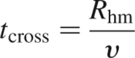
where Rhm is the half-mass radius of the cluster and υ is the velocity dispersion.
Our second time-scale is the relaxation time, trelax. As the stars and brown dwarfs move within the cluster they will undergo gravitational interactions with each other. The relaxation time refers to the period taken for a star to undergo sufficient interactions with various other bodies exchanging energy and have a resultant change in velocity of order |δυ|=|υ|. One may estimate the relaxation time of a cluster based on the two-body relaxation time as defined in Binney & Tremaine (1987):
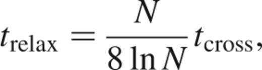
where N is the number of stars within the cluster.
The exchange of energy during the two-body interaction is a very important driving force for the cluster. During an interaction between two stars, energy is transferred from the heavier to the lighter one, until the cluster reaches a state of equipartition of energy. This results in the heavy star falling deeper into the cluster potential, namely toward the core of the cluster. This leads to the phenomena of mass segregation, whereby one finds the heaviest stars within a cluster migrating toward the core regions. Bonnell & Davies (1998) demonstrate that the time-scale for mass segregation within a cluster is well fitted by trelax (as was predicted by Spitzer 1940). Hence systems which are older than their trelax should be mass-segregated.
Whilst the heavy stars have lost energy during two-body interactions, the lighter stars (or brown dwarfs) have gained energy. As a result, the velocity of the body naturally increases and so it can move further out into the cluster. After a sufficient number of interactions, it is possible that the light star, or brown dwarf, may have a velocity which exceeds the escape speed of the cluster. This leads to the process of evaporation, whereby the cluster may lose mass via the escape of energetic stars.
2.2 Binary population dynamics
Within the cluster environment there is likely to be a population of binaries. These will provide another important mechanism for driving the evolution of the cluster; interactions between binary systems and single stars provide another method of energy transfer within the system, as we now briefly describe.
There are two types of binary system, hard and soft. The definition of hard and soft arise when a binary system undergoes an interaction with a third star. We have to consider the ratio of the total kinetic energy of the three bodies and the binding energy of the binary. If the kinetic energy of the system is greater than the binding energy, then there exists the possibility that energy can be passed into the binary and cause it to break up; this is referred to as a soft binary system. On the other hand, if the kinetic energy of the three-body event is less than the binding energy of the binary, the binary is said to be hard. In this case, energy is transferred to the interloping star and the binary becomes tighter, or harder. This transfer in energy then alters the energy budget of the cluster. The dividing line between the hard and soft regimes occurs when the total kinetic energy is just equal to the binding energy of the binary, and so leads to the definition of the critical velocity;
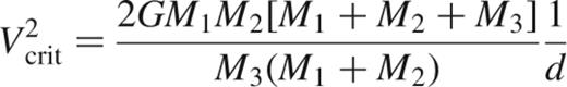
where M1, M2 are the masses of the two stars within the binary system and M3 is the mass of the third star, and d is the binary separation. If we equate the resulting kinetic energy of the system to the binding energy of the binary system, we can find the resulting definition of the hard–soft boundary limit:
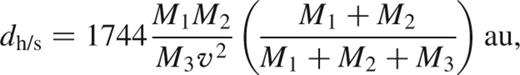
where v is now simply the relative velocity of the interloping star in km s−1 and the masses are in solar units. Clearly we now see that the hard–soft boundary of a star is now a function of the mass of the interloping star. Thus a system might be hard to one interaction whilst being soft to another one.
As already mentioned, if a hard binary system were to undergo an interaction, it is expected to get harder; in doing so energy has to be transferred from the binary system to the third star. This results in an increase in the velocity of the third star, and can ultimately lead to its evaporation from the cluster. Alternatively, if the interloping star has a mass greater than one of the components within the binary, then the two may be exchanged, with a hardening of the new binary system. A trivial calculation, based on a binary system with components of 0.6 M⊙ and 0.05 M⊙, undergoing an interaction with a 0.4 M⊙ star and forming a new binary which is ≈20 per cent harder than the original system, results in a kick velocity to the 0.05-M⊙ body (a brown dwarf) of 4.9 km s−1. The escape velocity of our clusters is of the order of 2.5 km s−1, so clearly if such an interaction were to take place, the ejected brown dwarf would soon escape from our cluster.
The interaction time-scale for bodies within the cluster may be defined as:
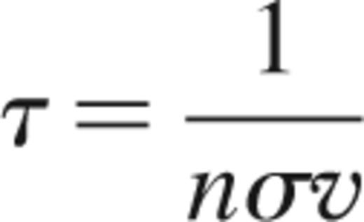
where n is the number density of stars, v is the relative stellar velocity and σ is the interaction cross-section. The clusters within our simulations all initially have a constant velocity dispersion, which is allowed to evolve with the cluster. As a consequence, the interaction cross-section may be estimated as:
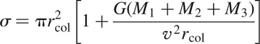
where v is the relative velocity of the binary and the interloping stars and rcol is the distance of closest approach for the system.
As stellar clusters evolve they are subject to tidal forces from the galaxy within which they reside. These forces will lead to perturbations on the orbits of the stars within the cluster. For simplicity, we model the motion of clusters moving on a circular orbit about the centre of our galaxy at a radius equivalent to that of the Sun from the Galactic centre (RG=8.5 kpc), this yields Oorts constants of A=14.5±1.5 km s-1 kpc-1 and B=-12±3 km s-1 kpc-1. With the addition of tidal forces to the calculations, the equations of motion for the stars within the cluster become (Giersz & Heggie 1997);
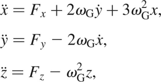
y¨=Fy-2ωGx·,

where ωG is the angular velocity about the centre of the galaxy defined by:
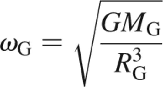
with MG is the mass of the galaxy contained within a distance RG.
One of the most obvious effects of the tidal field is the existence of a tidal radius for the cluster. This is the point at which the gravitational forces due to the cluster and the galaxy balance; it is defined by
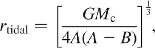
where Mc is the total mass of the open cluster. Once past this radius a star is no longer considered to be bound to the cluster and moves off to become a part of the galactic disc. Throughout all the simulations the effects of an external tidal field on the cluster are included with tidal radii calculated with the Oort constants as measured in the solar neighbourhood.
3 Initial conditions
3.1 Stellar population
Stellar masses for the population of stars within the simulations were produced by two methods. The first method was to simply utilize a catalogue of stellar masses for the objects currently present within the Pleiades. To this catalogue we added a population of 100 low-mass stars which were simply produced by doubling up the population of low-mass bodies in the catalogue. This allowed us to model the well-studied inner portions of the cluster. The addition of a further 100 bodies was decided on via numerical experiments that we performed.
The second method of producing stellar masses was to use the mass function by Kroupa, Tout & Gilmore (1993). With this function we produced a distribution of stars with an upper limit on mass of 10 M⊙ and a lower mass of 0.08 M⊙ (the hydrogen-burning limit). Evolution of the stellar population was accomplished via the use of fitting formulae (Eggleton, Fitchett & Tout 1989). In using the IMF by Kroupa et al. (1993) we extended our investigations by looking at clusters of different masses, with stellar numbers ranging between 1000 and 3000.
In addition to examining two different mass profiles we also investigate the effects of two different initial density distributions. The first is the Plummer distribution pattern which is commonly used in N-body simulations because it's simple and fairly realistic. The second set of models examined the evolution of a uniform spherical distribution, which is preferred by some authors (e.g. de la Fuente Marcos & de la Fuente Marcos 1999) as a model for open clusters.
3.2 Brown dwarf population
Within our simulations we added to the cluster a population of 1500 brown dwarfs, each of which have a mass of 0.05 M⊙ and positions and velocities determined in the same manner as for the stellar population. Investigations were made into using brown dwarf IMFs and populations of constant masses other than 0.05 M⊙; however, the choice of brown dwarf mass had very little effect on the evolution of the cluster or on the brown dwarf populations themselves.
3.3 Binary population
Within the simulations performed, between 0 and 500 primordial binary systems were added to the cluster. The binary systems were composed of stars already contained within the cluster, thereby conserving the total mass of the cluster between the simulations. In the cases where the Pleiades masses have been used the components of the binary systems have been randomly paired (Leinert et al. 1993, Kroupa, Petr & McCaughrean 1999, Kroupa 2000, although for a differing view see for example Mazeh & Goldberg 1992). For the other simulations, the IMF used produced the required binary components. In each simulation a discrete fraction of the binary population was forced to have a brown dwarf as a secondary. Three numbers which result from this treatment are the fraction of stars in binary systems, fs, the fraction of brown dwarfs contained within binaries, fbd and the fraction of objects (i.e. brown dwarfs and stars) contained within binaries, fbin:
where Ns, Nb, Nbd and Nbd,bin are the number of single stars, the number of stars contained in binary systems, the number of brown dwarfs and the number of brown dwarfs contained in binary systems. The various fractions considered are listed in Table 1. These were chosen so that we might investigate the effects that the different binary populations had on the evolution of the cluster.
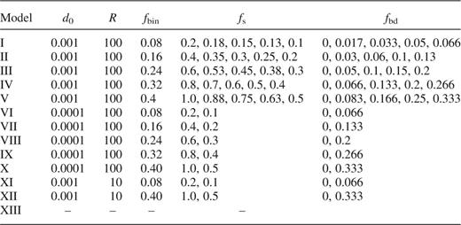
Properties of the binary systems in some of the simulations. Here R is the range used within the simulation to determine the binary properties, fbin, fs and fbd are the fractional numbers of objects, stars and brown dwarfs contained within a binary population. The separations quoted are in model units.
The positions of the binary systems were set to be consistent with the distribution of stars in the particular cluster. The eccentricities of the systems were selected from a thermalized distribution (Jeans 1929), whilst the nodes and inclinations were randomly selected.
The separations of the binary components were chosen so that they were uniformly distributed in log d. This was accomplished using the following;
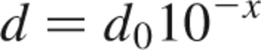
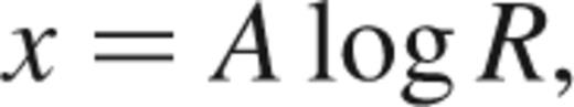
where d0 is the upper limit of the binary separation, A is a random number chosen from a uniform distribution between 0 and 1 and R is a quantity known as the range. The range determines the spread in binary separations between the upper limit and d0/R. A low value of R constrains the majority of the binary population to tight orbits whilst a high value leads to a greater spread in d. Both scenarios of high and low R were examined for the clusters in these simulations.
The separation of the binary components helps to determine what happens during a binary single encounter. When a tight binary undergoes an interaction, the energies involved tend to be much higher than during a corresponding interaction with a wide binary. However, the probability of a tight binary undergoing an interaction, is much lower than that of a wide system; this is simply because it presents a much smaller cross-section of interaction. To investigate the possible differences between the tight and wide systems, two distinct upper limits on the binary separation were examined within the simulations. One, with d0=90 au, produced a tight population of binaries whilst the other, d0=900 au, produced a wider set (both with R=100). Interactions involving the tighter binary population should lead to a change in the energy makeup of the cluster. Either the population will harden or the lighter member of the binary system (which could be a brown dwarf) will be ejected with a substantial velocity which may be sufficient for it to escape the cluster. Interactions involving the wider binaries are more likely to result in the ionization of the binary system. The associated kicks given to the binary components will be less than in the previous scenario. Consequently, it is possible that brown dwarfs released from these soft systems remain within the cluster. Our upper and lower limits on d allow us to investigate two important scenarios and see what effect they have on the evolution of the brown dwarf population. Some argument could be made for selecting an even larger upper limit for the separation of the binary components. Work by Gizis et al. (2001) demonstrates that the population of very wide systems (d>1000 au) is non-negligible; however, our separations should allow us to investigate the interesting effects within the cluster.
Table 1 details the properties of the binary populations within the simulations we have run.
3.4 Length scales in the N-body code
Within the N-body code there exists a characteristic length scale ℛ. This is a quantity which is fed into the simulation at the start and then all length scales during the simulation are scaled by this value. This distance maybe linked to the characteristic length scale associated with the Plummer model, b, which gives the space density as a function of radial distance from the centre of the cluster as:
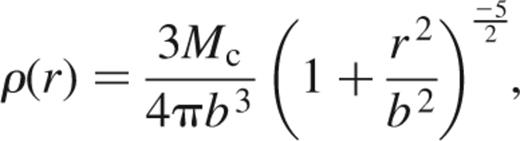
via the formula (Anderson 2001):
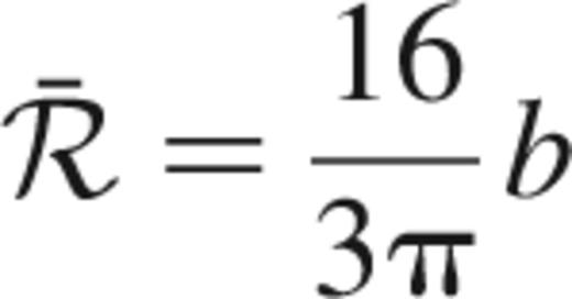
During the simulations detailed values of ℛ between 1.0 and 6.0 pc were investigated for both types of distribution pattern.
4 Numerical results
4.1 Overall evolution of the cluster
We begin by giving a brief overview of our results before giving a greater discussion about each of the salient points.
Through our simulations we have found that the presence of a brown dwarf population, regardless of their individual masses or numbers, has a minimal impact on the evolution of the cluster as a whole. More massive stars experience mass segregation towards the centre of the cluster, whilst the lighter stars and brown dwarfs move to the outer parts of the cluster.
As the lighter stars and brown dwarfs move outward, some fraction of them gained a sufficient velocity to escape from the gravitational potential of the cluster. Clusters which were initially more centrally condensed (i.e. those with small values of ℛ) had higher velocity dispersions and as a result evaporated faster than less tightly bound clusters (i.e. those clusters with large values of ℛ).
For all the models investigated, we found that during the early part of the cluster evolution (a few tcross) the escape rates of brown dwarfs was virtually identical to that of the low-mass stars. At later epochs some difference in the two rates would present itself; however, this was dependent on the binary fraction of the simulation as we shall discuss later.
We also found that both the initial density distributions evolve toward a similar state. That is to say, that the clusters that we initially set up with a uniform density rapidly evolved (within a few tcross) to a state similar to the equivalent Plummer model system. The major difference between the two initial density distributions relates to the number of bodies within the cluster at a given time. It was found that the Plummer model tended to undergo an early phase of mass loss where a fraction of the cluster was lost; however, this rapid loss only took place for a short period of time. Past a few tcross the loss rates for the two distributions became essentially equivalent, which is not overly surprising given the evolution of the uniform sphere and the Plummer models toward a similar King Profile.
Examinations of various cluster sizes demonstrated that the evolution remains the same qualitatively; however, the time-scales over which the processes occurred showed variation with the initial cluster properties. Clusters with smaller values of ℛ took a shorter period (in years) to evaporate and tended to evaporate more uniformly, with stars and brown dwarfs being lost at roughly the same rates. For ℛ values below 4, the loss of brown dwarfs from the Plummer and spherical model clusters were virtually identical; however, for larger ℛ values the Plummer models tended to lose roughly twice as many brown dwarfs as the equivalent spherical system at early cluster ages.
The first diagnostic commonly used to observe cluster evolution within a simulation is to look at the process of mass segregation. Fig. 1 shows how three different mass bins contribute to the make up of four shells within the cluster, as a function of time. The three mass bins considered were 0–0.05, 0.05–1.0 and M>1 M⊙. As can be seen, initially all three mass bins are evenly distributed within the cluster; however, mass segregation is seen to take place rapidly.
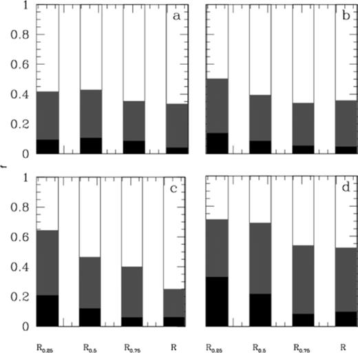
Plots of how the populations of stars within a given region change as a function of time. The above plots show how three different mass bins contribute to the make-up of a region. The black part of the histogram represents the heavier stars M≥1 M⊙, the grey represents the lighter stars of the cluster 0.05<M<1 M⊙ whilst the plain area represents the brown dwarf population of the cluster. The four regions considered were all fractions of the tidal radius, RT. Namely, 0≤R0.25<RT/4, RT/4≤R0.5<RT/2, RT/2≤R0.75<3RT/4 and 3RT/4≤R<RT. The four boxes represent, (a) the initial dispersal, (b) the dispersal after ≈125 Myr (≈10tcross, the age of the Pleiades), (c) ≈300 Myr and (d) the dispersal after 650 Myr (≈43tcross, the age of the Hyades cluster).
By the time the cluster has evolved to the age of 10tcross (which in the case of a cluster with ℛ=4.5 is 125 Myr, the age of the Pleiades cluster), we already see an increase in the fractional number of large-mass (i.e. M≥M⊙) stars within the inner parts of the cluster, with a corresponding decrease in the fractional numbers of brown dwarfs. In the outer parts of the cluster, however, there is a build up in the number of brown dwarfs.
This pattern continues on throughout the lifetime of the cluster. The last of the four plots represents the cluster when it has reached an age of ≈43tcross. Here we note that the fractional number of heavy stars appears to increase over the entire cluster; what is really happening is that the lighter stars and the brown dwarfs are being lost preferentially to the heavy stars and so the fraction of heavy stars within the cluster, as a whole, is seen to increase.
Fig. 2 shows how the number of brown dwarfs and stars contained within the cluster varies as a function of time for a simulation which initially contained 500 primordial binary systems, each of which had a brown dwarf as a secondary. These two figures help us to understand the apparent increase in the heavy star population present in Fig. 1. At the start of the simulation the normal stars are outnumbered 3:2 by brown dwarfs; consequently the heavy star population initially makes up a very small fraction of the entire population. However, when the cluster is ≈35tcross old we see that there is a near 1:1 relation between the brown dwarf and star numbers. Thus the fractional number of heavy stars within the cluster will have increased.
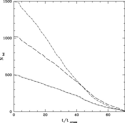
Evolution of the populations of the stellar and brown dwarf populations within a simulation that contained 500 primordial binaries, each of which had a brown dwarf as the secondary, i.e. a simulation where fbd=0.333 (see Section 3.3 for a full definition of fbd). The dot-long-dashed line represents the single population of brown dwarfs and the long-dashed line represents the population of single stars. The dotted line represents the brown dwarf population which is contained within a binary system with another cluster member and finally the dot-short-dashed line represents the stellar population contained within binary systems. Note that the number of objects in this figure are cumulative, i.e. there are 500 brown dwarfs tied up in binary systems and a further 1000 free brown dwarfs at the start of the simulation.
Another interesting feature that we note in Fig. 2 is a ‘repletion’ effect in the single body population of the cluster at around 40tcross. At this point, a number of binary systems are broken up, leading to a decrease in the binary population of the cluster, but to an increase in the number of single bodies. Thus there exists a method of re-populating the brown dwarf population in a cluster. In the case detailed, the number of freed brown dwarfs is fairly low. We shall discuss this effect in more detail in Section 5.2.
Another useful diagnostic of cluster evolution is to look at the variation of the core radius. This may be achieved via the equation of Casertano & Hut (1985);
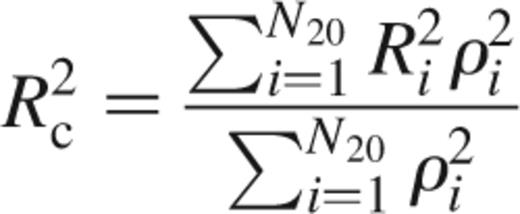
where Rc is the core radius, Ri is the radius to the ith star in the summation and ρi is the mass density around the ith star, not including itself. The summation is performed over the innermost 20 per cent of bodies. This relates, to within 6 per cent, to the observed core radius as defined by King (1962).
We performed a separate analysis for four distinct mass bins within the cluster. These are shown in Fig. 3. The core radius of the heavy stars (M≥2 M⊙ is denoted by the dotted line and, as can be seen, it decreases from its initial value as the stars sink toward the deepest parts of the cluster potential. The brown dwarfs (solid line) in contrast have a core radius which increases with time. This corresponds to their outward motion, following interactions with heavier bodies. Between these two extremes we see that the overall trend is for an increased core radius, with stars gradually moving out from the cluster centre before they eventually evaporate from the environment.
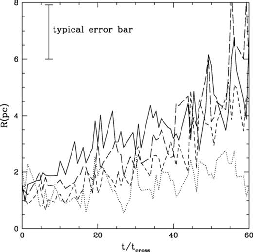
The time-averaged variation of the core radii (in pc) for the brown dwarf population (solid line) and various stellar populations. The dotted line represents the heaviest stars within the cluster, with a mass greater than 2 M⊙. The shortest dashed line represents stars with a mass between 1 and 2 M⊙, whilst the longer-dashed line represents stars with masses between 0.6 and 1 M⊙. The rest of the stellar population hasn't been plotted, for diagram clarity. However, it followed the general trend of the low-mass stars and brown dwarfs. Error bars in this and all other plots are the standard deviation errors (1σ) between different realizations of a particular set of cluster parameters. The error bar plotted in this figure may be regarded as the typical error on each data point. Variation from this value is less than 0.3 pc.
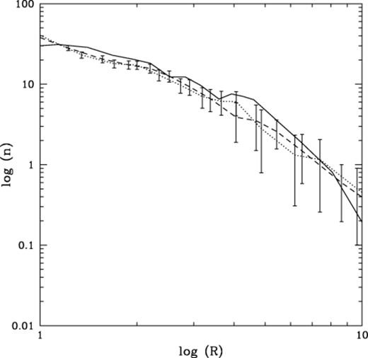
An important diagnostic for our investigation is to look at the surface density profiles of the brown dwarfs. Fig. 4 shows the profiles for two simulations once they had reached an age of 10tcross (equal to the age of the Pleiades). Both of these simulations contained 500 primordial binary systems; one set of binaries contained only stellar members, whilst the other simulation had a brown dwarf secondary in all of the systems. This second simulation is denoted by the dashed line on Fig. 4. As can be seen, within the core regions of the cluster the brown dwarf surface density is much increased in comparison to the non-brown dwarf containing binary population. However, when the brown dwarfs that were contained within the binary systems are removed from the data and the profile is re-plotted, we see that the density peak is much lower. This indicates that the brown dwarfs are actually being dragged towards the core of the cluster by their heavier primaries. In essence, the binary system may be regarded as a single body with a mass equal to the sum of its two components and an interaction cross-section given by the binary separation. Thus we expect the systems as a whole to experience mass segregation and sink toward the deeper part of the cluster potential.
A comparison of the brown dwarf surface density profiles (number pc−2) as a function of the cluster radius R (in pc) at the age of the Pleiades. The solid line represents the profile of a cluster which contained 500 primordial binaries, none of which had a brown dwarf member. The dashed line represents the profile of a cluster which contained 500 primordial binaries, each of which had a brown dwarf member. The dash-dotted line is for the same cluster, but this time the binary brown dwarf components have been removed from the analysis.
Another important quantity to consider within our simulations is the escape rate of both stars and brown dwarfs. It is found that the escape rates of stars remains largely unchanged by an increase in fbin with typical values of between 10 and 35 per cent of the initial members lost by an age of 10tcross. However, the loss rates of brown dwarfs do show a strong correlation to the values of fbin and fbd. If we simply increase the value of fbin keeping fbd low, even zero, then we see an enhanced ejection of brown dwarfs over that of normal stars. However, if we increase fbd at the same time, then this enhancement can be suppressed.
To understand the discontinuity in escape rates for the different simulations, we must consider the time-scale over which an interaction between a binary system and a single body will lead to the exchange of a body or the splitting up of the binary, tenc. For a binary system that is at the hard–soft boundary, this time-scale turns out to be well matched by the local relaxation time-scale, trelax; however, for a binary system with a separation much less than dh/s we find tenc≫trelax. Within our simulations, a number of the binaries containing brown dwarfs are hard to an interaction with an intruder of 0.6 M⊙. Hence, we expect the brown dwarf binary population to exist within the cluster for a period in excess of the relaxation time. This then explains why we see a higher population of brown dwarfs within the high fbd clusters at later cluster ages.
We also find that the escape rates of both the stars and the brown dwarfs are dependent on the initial cluster size and the cluster distribution pattern. As is expected, clusters which had smaller values of ℛ evaporated in a shorter period (in years) compared to clusters with larger values of ℛ. For clusters with an ℛ less than 4, the evaporation rates of the Plummer and uniform distribution patterns were almost identical; however, for larger values of ℛ it was found that the Plummer models underwent an enhanced mass loss at early cluster ages (10–15tcross) relative to the same size uniform distribution pattern. At later cluster ages the loss rates for the two models become more even; however, the Plummer model is obviously more depleted than the uniform model.
4.2 Comparison to the Pleiades cluster
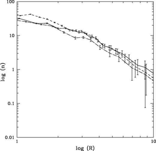
A comparison can be made between the properties of some of our simulations and the Pleiades cluster. We make a comparison between the Pleiades and our simulations which had an ℛ of 4.5 pc. Perhaps the most obvious comparison is shown in Fig. 5. In this figure we compare the stellar surface number density profile of the Pleiades cluster to that of a simulation containing 100 binary systems, each of which was made up of two stars, and another simulation which also had 100 binary systems but with each of these containing a brown dwarf as a secondary. As can be seen, over the majority of the cluster, the three profiles match remarkably well, with the only region where the simulations show an appreciable difference being the core.
A comparison of the surface stellar density (all masses), n, as a function of radius for the real Pleiades cluster (solid line) and two simulations. Both the simulations contained 100 primordial binaries; the dotted line had both members of the binary system as main sequence stars, whilst the dashed line represents a cluster where all the binary systems had a brown dwarf component.
In Table 2 we make a comparison between the properties of some of our simulations and data for the Pleiades cluster. As can be seen, we closely match many of the physical parameters describing the cluster, in particular the core radius and the crossing times. In Table 3 we list some properties of other nearby open clusters for comparison.
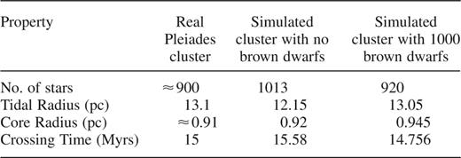
Table of the physical quantities of the real Pleiades cluster, along with two of the computer simulations when they had reached a similar age. Note that the core radius for the Pleiades cluster is actually that for stars with masses between 3 and 12 M⊙ and so is slightly less than the figures quoted for the simulated environments, which look at the cluster as a whole.
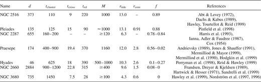
Table listing the physical properties of some of the nearby open clusters. The individual columns describe; the distance to the cluster in pc, d; the age of the cluster in Myr, tcluster; the half mass relaxation time of the cluster in Myr, trelax; estimated total mass of the cluster in M⊙, M; the tidal radius in pc, rtide; the core radius in pc, rcore. The penultimate column lists the fractional number of brown dwarfs left within our simulated clusters when they had reached an age equivalent to that of the real cluster, whilst the final column gives references to papers where information has been gathered from. Columns 2 through to 7 are adapted from Portegies Zwart et al. (2001).
4.3 Future evolution
Evolution of the cluster beyond the age of the Pleiades (≈10tcross; for ℛ=4.5 this is equivalent to 125 Myr) is shown on many of the figures presented in this paper. For instance in Fig. 1 we show the continuation of mass segregation. The lower right-hand panel shows mass segregation in the cluster at an age equivalent to the Hyades (≈43tcross≈650 Myr). As can be seen, by this epoch many of the stars within the inner regions of the cluster have a mass greater than 1 M⊙, whilst the brown dwarf population has primarily been exiled to the outer regions of the cluster.
Although we see an increased fractional number of heavy stars within the core regions of the cluster, we note that the total population of all bodies within this region actually declines over time. As time progresses, we are typically left with a few binary systems, containing relatively heavy stars in tight orbits, in the core region, whilst the rest of the stellar population moves outwards and eventually evaporates from the cluster.
Our most important result is regarding the evaporation of the brown dwarfs from the cluster. For the first few crossing times (10–15), the evaporation of brown dwarfs had been fairly similar to that of the lower mass stars within the simulation, with a loss of both types being in the region of 5 to 35 per cent. However, once past this point the ejection rate of the brown dwarfs may drastically increase. By 50tcross we observe differences between the two escape rates of up to 25 per cent in our most extreme simulations. This increased escape rate is linked to the interaction between the binary population and the single bodies in the cluster. Virtually all the binaries will be hard to an interaction with a brown dwarf and so the result of a brown dwarf binary encounter will be an increased velocity for the brown dwarf. This increased velocity will eventually lead to the evaporation of the brown dwarf from the cluster. We never completely lose all the brown dwarfs from the cluster; however, their numbers are drastically reduced in comparison to the stellar content.
5 Discussion
5.1 Evolution of the cluster
We have observed that mass segregation takes place within the cluster, with the brown dwarfs being moved out of the central regions of the clusters, to be replaced by heavier stars. Along with this mass segregation, we have also observed an enhanced escape rate for the brown dwarfs, compared to the stellar population, at later cluster ages.
This preferential escape rate, at older cluster ages, may be very important in explaining the lack of brown dwarf observations in older clusters, such as the Hyades, which is much closer to the Earth than the Pleiades, although this is not the only explanation for a lack of observations of brown dwarfs in old clusters, as we shall discuss later. The loss of many of the brown dwarfs relatively early in the evolution of the cluster would allow them to move many degrees away from the cluster of interest. A trivial calculation shows that a velocity of 1 km s−1, over a period of a million years, leads to a displacement of 1 pc. This being the case, if a brown dwarf is to be within, say, four tidal radii (which is ≈13 pc for the Pleiades cluster) then it can't have left the cluster any more than 52 Myr ago.
5.2 Evolution of the binary population
Within the cluster, some of the most important interactions will be between single stars and binary systems.
When a single star encounters a hard binary system the binary becomes harder and the released potential energy is converted to kinetic energy, for both the binary system and the single star. The kinetic energy given to the single star may result in it having a velocity which exceeds the escape velocity of the cluster; if this happens then the single star will eventually evaporate from the cluster.
An examination of the simulation data revealed that relatively few binary systems had undergone any significant interaction by the age of the Pleiades. A few systems did demonstrate signs of softening and a few had undergone an exchange interaction, whereby the lighter star in the binary was exchanged for a heavier intruder. The number of interactions and exchanges were dependent on the upper size of the binary, do, and the range, R, used. The number of exchanges was also dependent on the brown dwarf binary fraction fbd.
To understand why only a few binaries have undergone interactions by the age of the Pleiades, one needs to examine equations (5)) and (6. By rearrangement of these two equations and substitution of the cluster age, τ, one may obtain an expression for the maximum size of a binary that has yet to undergo an interaction;
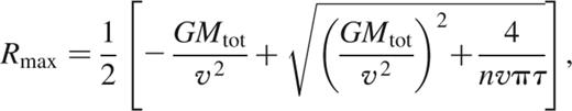
where Mtot=M1+M2+M3 and v is the relative velocity between the binary and the intruder star. As with the hard–soft boundary, we see that this is a function of the intruder mass. This formula assumes we have a constant velocity dispersion throughout the cluster. As the cluster evolves, this will no longer be the case and the formula will need to be modified. Any binary with a separation less than Rmax will not have undergone an interaction and so its properties should remain unchanged.
If we substitute properties appropriate to the Pleiades cluster into this formula, namely n≈150 pc-3, M1=M⊙, M3=0.6 M⊙ and v=2 km s-1, we obtain Fig. 6.
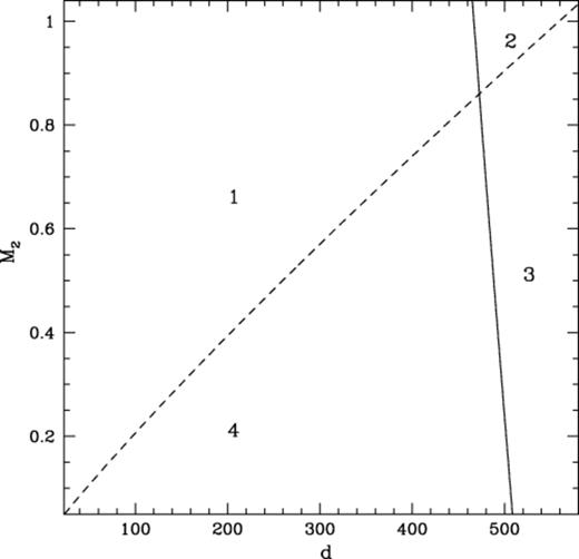
Comparison of the hard–soft boundary (dashed line) of a binary with the maximum size that a binary can have before it will interact with another star (solid line), both in au, for a variety of secondary masses (in M⊙). The plot is for a primary mass of 1 M⊙ with a velocity dispersion of 2 km s−1.
As marked, the figure may be broken into four distinct regions. The first region, region 1, extends from the y-axis up to the solid line (which represents the maximum size of a binary yet to undergo an interaction) and lies above the dashed line (which represents the hard–soft boundary); binaries which occupy this region may be regarded as safe within the cluster environment. Statistically, they shouldn't undergo an interaction within the cluster environment. The second region, region 2, denotes hard binaries that will undergo interactions within the time allotted. These interactions will lead to either a hardening of the binary or an exchange of members. The third region, region 3, represents soft binaries which will undergo interactions. These binaries will either become softer or be broken up. The fourth region, region 4, represents soft binaries which shouldn't interact within the period allotted.
We can investigate what equations (4) and (18) mean for the binary systems within our simulations. Fig. 7 shows a plot of the binary separations against the product of the two components masses; the different symbols used represent which region the binary systems occupy on Fig. 6. We show in this figure how the populations of two different simulations may be regarded at two different epochs, plot (i) and (ii) represent clusters at an age similar to that of the Pleiades cluster, whilst plots (iii) and (iv) are results calculated for a cluster with an age similar to that of the Hyades cluster. Plots (i) and (iii) represent a simulation where a primordial population of 500 binaries were forced to take a brown dwarf as a secondary, whilst plots (ii) and (iv) are representative of a simulation where again 500 primordial binaries were present but this time they were only made up of main-sequence stars. Both populations of binary systems were set up with an upper limit to their separations of d0=900 au and R=100. Within these four plots it is possible to reconstruct the four regions of Fig. 6. Within Fig. 7 the following symbols have been used to denote what region a binary system would occupy in Fig. 6: open triangles represent region 1, filled triangles denote region 2, filled circles are equivalent to region 3 and open circles denote region 4. The number of systems within each of these four regions is detailed in Table 4. In each plot a line has been drawn; this may be thought of as denoting the hard–soft boundary line of Fig. 6. It is then possible to see that the four different types of binary system are clumped together in distinct regions. This indicates that the ability of a binary system to interact is determined by its binding energy; the higher the binding energy, the harder the binary, and the less likely it is to interact. It can be seen that the number of binary systems that may be regarded as able to interact increases with time, just as one would expect from equation (18). However, it is interesting to note that the majority of systems may still be regarded as unable to interact even after a period of 650 Myr. When a system was split up by an interaction with a third star, the ejected star or brown dwarf typically had insufficient energy to escape from the cluster. As a result it in essence became a member of the free-floating population subject to the same conditions as all the other free objects within the cluster.
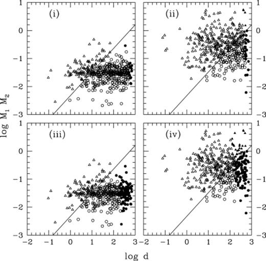
Demonstration of how the binary systems within two simulations may be regarded, in terms of equations (4) and (18), at different times (d in au, M1 and M2 in solar units). The top row represent clusters with an age similar to that of the Pleiades, whilst the lower row represents clusters at the age of the Hyades. Two separate simulations were considered. Plots (i) and (iii) represent a primordial population of 500 binary systems in which each of the systems were forced to have a brown dwarf as a secondary; plots (ii) and (iv) represent a population where the binary systems were only made up of main sequence stars. Open triangles represent binary systems which may be regarded as hard and non-interacting within the allotted time period and filled triangles denote binary systems which are hard and may interact within the given period. Open circles represent non-interacting soft systems and filled circles show soft interacting systems.
The splitting up of a binary containing a brown dwarf has interesting possibilities for re-populating the single brown dwarf contingent in the cluster. Within our simulations we have observed some evidence of ‘repletion’ late in a clusters evolution; however the numbers involved are very small and not likely to make an appreciable difference in our ability to see free brown dwarfs within the cluster. In theory, we might be able to ‘tune’ the binary separations, so that instead of following a description of being uniform in log d they have a peak in separations which cause them to all become able to interact at roughly the same time. In doing so we might be able to induce a sizable ‘repletion’ effect within the cluster. In actual observations this ‘repletion’ effect would be seen as an increased brown dwarf population compared to what we predict should be present at a given time.
5.3 Brown dwarf–brown dwarf binaries
Prompted by the discovery of several brown dwarf–brown dwarf binary systems within the Pleiades cluster, a set of simulations were run within which a distinct fraction of the brown dwarfs were forced to be in a binary system with another brown dwarf, along with a population of binary systems composed solely of stars (model details in Table 5). This fraction, which we refer to as the double brown dwarf fraction, is defined so that;

where Nbd,bd is the number of brown dwarfs contained within a binary system with another brown dwarf. In all the simulations we kept the total number of binary systems constant.
The overall evolution of the cluster isn't effected by the population of brown dwarf–brown dwarf binaries; however, the number of exchanges within the cluster is sensitive to the value of f2BD. As the fraction of binaries containing only brown dwarfs rises, the number of interactions where one member of the binary system is replaced by a heavier interloper falls. This may initially seem contradictory, after all the binding energy of a double brown dwarf system is much lower than that of a similar system made up with a main sequence star; however, the reason for the decreased exchange rate lies within equation (18). Within this equation we see that the total mass of the system is important in determining the maximum size of a binary which has not yet interacted. This mass term arises because of the effects of gravitational focusing, whereby the mass of the binary system actually draws the interloping star toward it. In the case of a brown dwarf–brown dwarf binary system, the total mass of the binary is relatively low and so the effects of focusing are negligible. Consequently, the maximum size of a binary, made up only of brown dwarfs, not to have undergone an interaction at some epoch is much greater than that of a system which contains a main sequence star.
As a result we expect the binary population containing a brown dwarf to exist within the cluster environment throughout much of the lifetime of the cluster. The brown dwarf–brown dwarf binary presents possibly the best opportunity for detecting brown dwarfs. In such a system, we don't have to worry about glare effects because both components have roughly the same luminosity. Another advantage is that the pair of brown dwarfs will move on to the binary second sequence with a brighter apparent magnitude than a single brown dwarf, aiding their detection.

5.4 Binary system visibility
If we are to detect the two components within a binary system, an important consideration is their separation. With an HST angular resolution of 0.1 arcsec, one can trivially calculate the minimum binary orbit that we should be able to resolve; this turns out to be 13.5 au for the Pleiades cluster, which is 135 pc from the Earth. This is of course for a binary system lying perpendicular to the line of sight (i.e. an inclination of 0°). The natural inclination of the system to our line of sight means that many systems which have a separation of greater than 13.5 au are still unresolvable.
One can show that the fraction of circular binary systems visible despite the effects of inclinations is described by the formula:
where x is the ratio of the true binary separation to the minimum separation required for resolution.
If one were to consider our wider binary population (i.e. a maximum binary separation of 900 au), one can show that when observations are made of a cluster at the Pleiades distance with ground-based telescopes (which have their resolution limited to 1 arcsec by seeing effects in the atmosphere) approximately 65 per cent of the systems would remain unresolved into two distinct sources. The situation would become better with the use of the HST with approximately 14 per cent of the systems remaining unresolved; however, the cost in telescope resources means that this is most unlikely to take place.
In addition to the problems associated with inclination effects, there is another method of hiding a brown dwarf from direct observation within a binary system. The low luminosity of a brown dwarf means that it is possible to hide it via the glare of the primary. A reasonable estimate for the difference in fluxes that would prevent resolution of two distinct components is of order 10:1. This problem can be overcome to some extent by making observations within infrared bands where brown dwarfs emit much of their energy, for instance in the K band, thus ensuring the highest ratio of fluxes possible. With the 10:1 constraint on the relative fluxes, it is possible to calculate the required angular separation between the two components of a binary system if they are to be resolved optically. For a low-mass main-sequence dwarf as the primary, the minimum required angular separation is of order 0.7 arcmin for a heavy (0.07 M⊙ brown dwarf and is of order 2.35 arcmin for a lighter (0.01 M⊙), hence cooler, brown dwarf. Whilst for a primary like the Sun the minimum angular separation for a heavy brown dwarf and the primary is 1.35 arcsec and for the lighter brown dwarf it is 2.65 arcsec. These angular separations can then be interpreted in terms of the minimum physical separation between the binary pair. Clearly in the case of our softer binary population (upper separation of 900 au) located at the distance of the Pleiades, observations with a ground-based telescope would then only resolve between 12 and 27 per cent of the entire binary population.
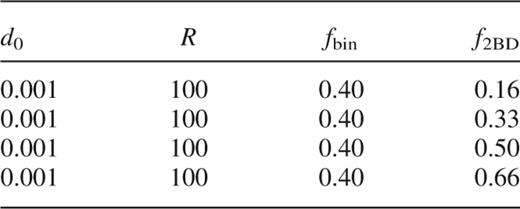
Details of the additional runs performed (along with those detailed in Table 1), to investigate the effects of a population of binaries made up solely of brown dwarfs. Within the table, d0 is the maximum separation between the binary components, R is the range of the binary orbits i.e. it defines the spread in binary orbits – see Section 2.2 for full details. fbin is the fraction of objects within the cluster that are contained in binaries, and f2BD is the fraction of brown dwarfs contained within binaries with other brown dwarfs.
Even if the binary systems are not directly resolvable, it is still possible to discover the existence of a population of binaries. The main method of detecting an unresolved population is to look for the existence of a binary second sequence in the colour–magnitude diagram of the cluster, as we shall discuss in the next section.
5.5 Brown dwarf cooling and the binary second sequence
Brown dwarfs have no renewable source of energy; that which they radiate comes from reserves built up during the original accretion from the nebula and subsequent contraction. As a result, brown dwarfs are continually cooling down; this means that they are becoming gradually dimmer.
This cooling is important in hiding brown dwarfs from sight. There are a number of papers describing models of brown dwarfs, for example Baraffe et al. (1998). They find that a 0.05-M⊙ brown dwarf will have a magnitude in the I band of 19.56 at the age and distance of the Pleiades cluster; this is still within the limits of most modern surveys. However, if one were to take into account the spectrum of brown dwarf masses resulting from the tail of the IMF, one finds that the Pleiades observations, with a limiting I-band magnitude of 20 (which corresponds to a lower detectable brown dwarf mass of ≈0.04 M⊙), will fail to detect some 50 per cent of the brown dwarf population (assuming brown dwarfs have masses between 0.02 and 0.075 M⊙ described by the IMF of Kroupa 1995). In the case of the older Hyades cluster (≈650 Myr) the fraction of brown dwarfs missed by a similar survey would be about the same, the greater brown dwarf age off set by the clusters proximity to us. More recent surveys extend the depths of observations through to I=22, in the case of the Pleiades and Hyades this should result in only ≈35 per cent of the brown dwarf population being missed.
The previous arguments can only be applied to isolated brown dwarfs. Those within a binary system will be subject to different conditions. As was mentioned in the previous section, the presence of a binary population, which isn't directly resolvable, may be betrayed by the existence of a second sequence on the colour–magnitude diagram.
A binary system has a luminosity equal to the sum of the two components, but a colour which is redder than the equivalent star of the same luminosity (Haffner & Heckmann 1937, Hurley & Tout 1998). This leads to the formation of a second sequence lying ≈0.75 mag above the main sequence on the colour–magnitude diagram. This relative height of the second sequence is true for binary systems with non-extreme mass ratios (q=M2/M1); however, in the cases where brown dwarfs are the secondary, an extreme mass ratio is likely to occur. These systems tend to move away from the second sequence and occupy the gap between it and the main-sequence line.
If the mass ratio is particularly extreme, then the redness of the low-mass companion is insufficient to move the system on to the second sequence. In this case the system lies either somewhere between the two lines or very close to the main sequence. The most extreme mass ratio that one expects to find lying on the second sequence is of the order of q=0.33 (this is within the I, I–K plane; Steele & Jameson 1995). If q is less than this, the binary moves away from the second sequence. In the case where a brown dwarf is the companion, a low value of q is quite probable, unless we also have a fairly low mass primary.
Clearly, even for a massive brown dwarf (≈0.07 M⊙), if the binary system is to lie on the second sequence then the primary can be no more massive than ≈0.2 M⊙. Within our simulated data we find that from all the binary systems still present at the age of the Pleiades, between 2 and 6 per cent fulfilled the condition of q≥0.33; clearly the vast majority of binary systems will not be detectable in this manner. As we have previously discussed, brown dwarfs cool as they get older. This results in their magnitudes becoming fainter, and as a consequence of this a system which was initially on the binary second sequence will move away from it. Thus, in old clusters, it is possible that a population of brown dwarfs contained in binaries may be entirely hidden from view.
Observations of the Pleiades cluster (Steele & Jameson 1995) have shown some evidence of a second sequence at very low stellar masses, thus indicating the existence of a brown dwarf population in binary systems.
5.6 Probabilities of finding a brown dwarf
We have detailed many methods by which brown dwarfs are lost from observations; these range from dynamical depletion to hiding the brown dwarf in a binary system. What do these losses imply for the probability of observing a brown dwarf within a cluster?
It is trivial to find out how many brown dwarfs are left in the various simulations at various epochs – a general trend shows that the more brown dwarfs which were initially contained within a binary systems, the greater the number still contained within the cluster at later epochs. However, it is not merely a question of how many brown dwarfs are present within the cluster, but rather how many can be seen. As we have said, at later epochs there tends to be a higher number of brown dwarfs in the clusters which have a high fbd, this is because the brown dwarfs in binaries are retained by the cluster. Unfortunately, as we have discussed, a high proportion of binary systems are hidden via inclination effects. Despite this, one still expects to be able to see more brown dwarfs in these high fbd clusters at very old cluster ages compared to clusters which had fewer brown dwarfs initially contained in binary systems.
We see, in Fig. 8, that at the age of the Pleiades (≈10tcross), the simulated cluster still contains nearly 90 per cent of its original brown dwarf members. The most up-to-date observations, however, have only revealed 30 brown dwarfs within the real cluster (this is partly due to the fact that only a modest fraction of the whole cluster has been surveyed to the required depth to find brown dwarfs). In Table 6 we show the number of brown dwarfs that we would expect to see in our simulated cluster, if it were observed to the same depth and area coverage as the Pleiades currently is. When we look at a time closer to the Hyades age, 650 Myr (≈43tcross), we see that within the more pessimistic simulation where no brown dwarfs were contained within binary systems only ≈10 per cent of the original brown dwarfs are retained within the cluster. The most optimistic simulation indicated that, at the age of the Hyades, the cluster would contain only ≈30 per cent of the original brown dwarf population.
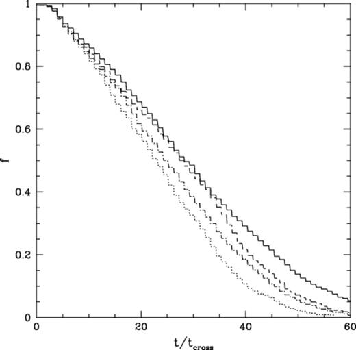
The fraction of the original brown dwarf population still contained within the cluster as a function of the cluster crossing time for a number of our simulations. The solid line represents a simulation containing 500 primordial binaries each of which had a brown dwarf secondary, whilst the short-dashed line is for a similar simulation, except that this time no brown dwarfs were in binary systems. The long-dashed line represents a simulation containing 100 primordial binaries, each of which has a brown dwarf secondary, whilst the dot-dashed line represents the same simulation, except no brown dwarfs were contained within a binary systems. All these simulations were performed with an ℛ=4.5.
Combination of the data within Fig. 8 and the various effects which hide brown dwarfs (i.e. cooling, being contained within a binary system), shows that at the age of the Pleiades (≈10tcross) anywhere between 40 and 50 per cent of the original brown dwarf population should, in principle, be viewable (this is with an I-band magnitude limit of 20; surveys limited to I=22 should be able to find up to 65 per cent of the brown dwarf population); whilst at the age of the Hyades (≈43tcross) this figure falls off to between 3 and 16 per cent. Thus, the probability of finding a brown dwarf in an old cluster like the Hyades is very small.
6 Conclusions
Through our simulations we have been able to match closely the observed stellar surface density distribution, as well as other key properties of the Pleiades cluster, for a varied number of brown dwarfs within the cluster environment. This indicates that the presence of a brown dwarf population is unlikely to be betrayed by the observed stellar population.
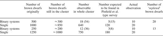
A comparison of the observable number of brown dwarfs contained within our simulated clusters and the current observations of the Pleiades cluster. In the case of the binary systems we have two figures quoted for the number of systems visible. The first refers to those which should be found via the binary second sequence as those found within the Pleiades have been. The second figure refers to those which should be resolvable. In both simulations there were initially 1500 brown dwarfs and 500 binary systems with a discrete fraction containing brown dwarfs (as detailed in the first column), the systems had an upper separation of 900 au. In the fifth column we detail the number of brown dwarfs that we would expect to find within a survey akin to that carried out by Pinfield et al. (2000). This survey covered a total of six square degrees spread over five separate regions within the central parts of the cluster. As can be seen such a survey dramatically reduces the number of brown dwarfs that we expect to see compared to a survey of the cluster as a whole.We see that such a survey performed on our simulated clusters would yield too few binary systems that contain brown dwarfs (found via the second sequence), whilst it would find too many single brown dwarfs when compared to observations of the real Pleiades cluster.
We have demonstrated that, in the case of the Pleiades and Hyades clusters, the cooling of the brown dwarfs on their own should be insufficient to hide them from view.
However, if they are contained within a primordial binary population, then the difference in luminosity between the primary and the brown dwarf companion might be enough to make the companion unobservable, as a result of equipment limitations. Observations lend credence to the existence of a primordial binary population within the Pleiades. In particular, the discovery of a binary second sequence by Steel & Jameson (1995) indicates that there are many unresolved binary systems within the Pleiades cluster, all of which have the potential to hide brown dwarfs. The work by Richichi et al. (1994) indicates that around half of the observed stars in the sky must actually be unresolved binary systems. This again lends credence to some of the high binary fractions used in some of our simulations.
Our multiple realizations of the cluster have shown that the effects of different brown dwarf binary fractions are minimal. The dynamics of the cluster remain largely unchanged, with key features such as the stellar surface density profile and the loss rates of stars remaining almost the same for a particular cluster size. Containing a contingent of brown dwarfs within a primordial binary population has two key effects; first, the larger this contingent, the greater the population of brown dwarfs present within the cluster at later cluster epochs. Secondly, by containing the brown dwarfs within a binary system we have an effective method of hiding them from view, both in terms of inclination effects and their continual cooling.
In the case of the Pleiades cluster we have demonstrated, via the combination of Figs 4 and 8, that the effects of dynamical depletion of brown dwarfs is insufficient to explain the low number of single brown dwarfs observed in the well-studied central portions of the cluster (≈30 strong brown dwarf candidates in total, a third of which are in binary systems with low-mass companions). However, in the case of the much older Hyades cluster, depletion effects become far more important, with perhaps two thirds, or more, of the initial brown dwarf population lost from the cluster, and a greater proportion hidden from view by effects associated with binary systems. This quite clearly helps to explain why there are no confirmed brown dwarf sightings within the Hyades cluster.
Of concern, however, is the relatively low number of brown dwarf observations within the well-studied central portions of the Pleiades cluster. The data from our simulations would seem to indicate that the surface number density of brown dwarfs within the central parts of the cluster would lend themselves to detection. This being the case, there are a number of possibilities for explaining the disparity between observation and our results, as follows.
(i) The number of brown dwarfs within the cluster has been overestimated. This seems likely, as the work of Rabound & Mermilliod (1998) demonstrates the extreme uncertainties as regards the mass of the Pleiades cluster. They use three distinct methods of predicting the cluster mass; the use of the tidal radius, the virial theorem and a proposed IMF, and get three different results with very large confidence bands.
(ii) The cluster contains a population of very low mass brown dwarfs. As a result of their low mass these brown dwarfs have quickly cooled to a point below our detection threshold.
(iii) A greater proportion of the brown dwarfs are contained within moderately tight binary systems and so are not optically resolvable. Brown dwarfs contained in systems with a low-mass primary (such that the mass ratio of the system is greater than one third) will be detectable via the binary second sequence on the CMD. Brown dwarfs contained in systems with heavy primaries (M>0.2 M⊙) may be detectable via the radial shifts in the light from the primary, in much the same way as the search for extra-solar planets is being conducted.
It is this later theory that we favour. The observed number of single brown dwarfs compared to our predictions is so small it seems unlikely that such a large single population exists within the cluster. The effects of mass segregation cannot move a sufficient fraction of the single brown dwarfs out of the well-studied central region of the Pleiades cluster to account for the low numbers observed. We have shown that the majority of brown contained within a binary system are virtually undetectable without a massive search for radial shifts in the light of the primary. We also see that our simulated data predicts too few binary systems which would be observed on the binary second sequence; this would strongly suggest a much higher binary fraction within the cluster (which is of course necessary to explain the main-sequence star–star binary systems we observe as well), providing a method of hiding a substantial population of brown dwarfs within the cluster. Further, an examination of our simulations demonstrates that a considerable fraction of the currently single brown dwarfs may actually have initially been in binary systems which were broken up, i.e. the single population is, in part, made up by the ‘repletion’ effects that we discussed in Section 5.1. This would remove the need for a large single population of brown dwarfs to be present within the newly formed cluster.
Acknowledgments
TA gratefully acknowledges support through a PPARC research student ship. MBD gratefully acknowledges the support of the Royal Society through a URF.We are grateful to Sverre Aarseth for providing us with a copy of his NBODY 6 code.
References
