


Abstract
We present a deep multicolour CCD mosaic of the Coma cluster (Abell 1656), covering 5.2deg2 in the B and r bands, and 1.3deg2 in the U band. This large, homogeneous data set provides a valuable low redshift comparison sample for studies of galaxies in distant clusters. In this paper we present our survey, and study the dependence of the galaxy luminosity function (LF) on passband and radial distance from the cluster centre. The U, B and r band LFs of the complete sample cannot be represented by single Schechter functions. For the central area, 
 , we find best fitting Schechter parameters of
  and
and  ,
,  and
and  and
and  and
and  . The LF becomes steeper at larger radial distances from the cluster centre. The effect is most pronounced in the U band. This result is consistent with the presence of a star forming dwarf population at a large distance from the cluster centre, which may be in the process of being accreted by the cluster. The shapes of the LFs of the NGC 4839 group support a scenario in which the group has already passed through the centre.
Introduction
Clusters of galaxies are important laboratories for studies of galaxy evolution. The galaxy population in clusters is very different from the population in the field, suggesting that galaxy formation and evolution are a strong function of the environment.
The galaxy luminosity function (LF) should be an excellent tracer of environmental effects. Knowledge of the shape of the LF (in different bands) is a powerful tool for studies of galaxy evolution. Specifically, one can look for correlations between the shape of the general LF and environmental or cluster properties. In general the LF drops steeply at bright magnitudes and rises gradually at fainter magnitudes, as described by a Schechter function (Schechter 1976). Sometimes, however, features such as bumps and a steeply rising faint part are found, which cannot be fitted adequately by a single Schechter function. Galaxies in the cluster core region are expected to have a different merger history than the galaxies populating the cluster outskirts where the cluster blends into the field. This should be reflected in differently shaped LFs for dense and less dense regions within a cluster. López Cruz et al. (1997) propose that the flat faint end slopes found in rich clusters result from the disruption of dwarf galaxies. Biviano et al. (1995) report a dip in the bright part of the general LF for rich clusters which is not seen in LFs of poor clusters or in the field. Andreon (1998) verified the invariance of the shape of the bright part of the type dependent LF in a large range of environments from the field to the cores of clusters several orders of magnitude denser. The determination of the exact shapes of LFs is difficult as the faint ends suffer from uncertainties in the contamination by field galaxies.
The Coma cluster  , richness class 2) is the richest of the nearby clusters and ideal to study environmental effects (for a detailed overview of research on the Coma cluster see Mazure et al. 1998). Previous large field studies of the photometric properties of the galaxies in the Coma cluster have been based on photographic plates (e.g. Godwin, Metcalfe & Peach 1983; Lugger 1989). CCD studies yield better photometric precision, but have hitherto been limited to relatively small areas, mainly focused on the central regions (e.g. Thompson & Gregory 1993; Biviano et al. 1995; Bernstein et al. 1995; López Cruz et al. 1997; Secker et al. 1997; Lobo et al. 1997; de Propris et al. 1998; Trentham 1998a, b; Mobasher & Trentham 1998; Andreon 1999). We combine the benefits of wide field coverage with the photometric accuracy attainable with CCDs, by using the Wide Field Camera (WFC) on the Isaac Newton Telescope (INT) to image a large part of the Coma cluster from the dense core to the outskirts of the cluster. Our data offers the interesting possibility to study the LF for a large range of environments within the cluster. The primary goals of our survey are to study the LF, the colour magnitude relation and to complement a large Hi survey conducted with the Westerbork Synthesis Radio Telescope (WSRT).
In this paper we present our data and use our catalogue to construct U, B and r band LFs for various regions of the Coma cluster area. Our study complements previous studies of the LF of the Coma cluster by providing accurate, deep CCD photometry in three bands, covering an area of 5.2deg2. Our wide field U band data is of particular importance, because the  colour is a sensitive indicator of the presence of young stellar populations. Furthermore, the rest frame U band remains in the optical window out to
  , which makes the U band observations very useful for comparison to high redshift clusters. Previous U band studies of Coma were limited to small samples of individual galaxies (Bower, Lucey & Ellis 1992). Our mosaic has similar resolution (in kpc) and size (in Mpc) as large Hubble Space Telescope (HST) WFPC2 mosaics of high redshift clusters (e.g. van Dokkum et al. 1998) and provides a valuable low z zero point for studies of the evolution of galaxy morphology, colour and luminosity. For the first time a U band LF for such a large area of the Coma cluster is determined. In addition we study the dependence of the LF on passband and projected distance from the cluster centre.
Throughout this paper we use  and coordinates are given in equinox J2000.0.
Observations
The data were collected during the nights of 1999 March  with the WFC on the INT, on Rogue de Los Muchachos on the island of La Palma (Spain). The WFC consists of four
  EEV CCDs and a fifth CCD for autoguiding. The layout of the chips is shown in Fig. 1. It is designed to provide a large field survey capability for the prime focus of the INT. The sky coverage is
  with a plate scale of 0.333arcsecpixel−1. The camera covers 80 per cent of the unvignetted field of the INT.
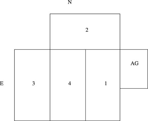
Layout of the four science CCDs and the autoguider CCD as used in our survey of the Coma cluster (rotator angle at 270°). The four science CCDs cover an area of  .
.
We have imaged a mosaic of 25 overlapping pointings covering a total area of ∼5.2deg2 or 
 . Broadband filters RGO U, Harris B and Sloan r were used for the six pointings covering the core and the south west group (containing NGC 4839). The other 19 pointings were observed with Harris B and Sloan r. Two exposures, offset by ∼1arcmin, were taken for each pointing. This ensured that we would be able to determine the relative zero point offsets between exposures and chips and there would be very few gaps in the final mosaic. Furthermore, galaxies in the overlapping regions give us good estimates of the errors due to photon noise and flat fielding. Integration times were
  in B,
in B,  in r and
  in U. The layout of the field is shown in Fig. 2. Thick lines delineate pointings which were observed in the U band, as well as in B and r.
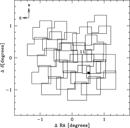
Layout of the 25 overlapping pointings covering an area of ∼5.2deg2. Thick lines delineate pointings which were observed in the U band, as well as B and r. Pointing 11 served as reference field for the photometric calibration. The position of NGC 4839 is indicated by the filled square. Coordinates are given relative to 
The overall weather was good, with an average seeing during the first two nights of ∼1.4arcsec and ∼1.9arcsec during the last two nights in the r band. The strategy was to observe the central parts of the cluster in U, B and r under photometric conditions. During the first night the standard Landolt (1992) fields Sa107 602 and Sa101 427 were also observed at similar airmasses to the central fields. These standard fields contain many standard stars and give a good spread over the four CCD chips. This is important for the absolute calibration, because no two chips have exactly the same characteristics. In fact it is known that the WFC is non linear.
The Coma fields were observed when the cluster had risen to an airmass <1.8. At the start of nights 3 and 4 we took exposures of an empty field (see Section 4.4). This field was later used to correct U band galaxy counts for foreground/background contamination.
Initial reduction
Flat fielding
Prior to any reduction, the images were inspected to judge their quality. For each chip the bias frames per night were checked for repeating structures and count levels. The bias structures were also visible in the science images. We combined all bias frames to create an average master bias frame for each night and each chip. After several tests we decided that the bias subtraction had to be performed in two steps; we first subtracted the overscan level by fitting a second order polynomial to the columns and then subtracted the (overscan subtracted) master bias frames. The second step successfully removed the remaining bias structures for chips 1, 2 and 4. Chip 3 suffered from a few bad columns. These were removed by interpolation or by aligning and combining the images taken with a small offset. The rms noise level in the master bias frame was negligible compared to the rms noise in the science frames.
Accurate flat field images were created from the science frames. We have obtained 52 science images of the Coma area per chip per band for the B and r bands. For the U band we have 23 science images, including the empty fields. We constructed a B and r band master flat by scaling these images by the mode, rejecting the lowest 10 and highest 15 pixel values, followed by median filtering. The U band master flats were constructed in the same way, but there we rejected the lowest five and highest 10 pixel values before median filtering.
As a test we compared our flat fields to the ones of the Wide Field Imaging Survey which are available from the WFC archive.2 Differences between the flat fields were at the level of 10−4 or less, assuring that we have good quality flats.
After flat fielding, approximately 2.5 per cent of the area of chip 3 still suffers from ∼3 per cent variations in the background, because this chip is partly vignetted. Because of the overlap between neighbouring pointings, this has very little impact on our final mosaic. On average the images are very flat, with less than 0.8 per cent variations in the background.
Photometric calibration
The ultimate aim was to obtain a homogeneous photometric scale over the whole area covered. We dedicated the photometric anchor point to be chip 4 of pointing 11 (Fig. 2) at airmass 1.000. This field was observed during the first night under photometric conditions at a time close to when the standards were taken. First, we determined the photometric offsets between the four chips of the WFC, using objects in overlapping regions between the two offset exposures for each pointing. For the U band, the number of bright objects in overlapping areas was low. Therefore, we could not use objects to determine the offsets, because this would have given unreliable results. Instead, we used the sky level to determine photometric offsets. First, we made sky images by filtering out all objects of the science images in the same way as for the flat fields. Comparison of the mean sky levels of the sky images gave the offsets. The resulting offsets are listed in Table 1. Errors indicate the uncertainty in the mean of all the independent measurements. The 1σ spread between independent measurements of pairs of different pointings is much larger, and is caused by varying conditions between observations of neighbouring pointings. The offsets depend on the passband, because the response curves of the four CCDs are not identical.
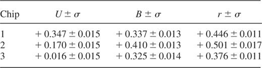
Photometric offsets relative to chip 4.
We applied these offsets to bring all chips to the same scale. Only the first two nights were photometric and we proceeded by determining the photometric offsets between neighbouring pointings. The mean offset values are based on the eight (or more) brightest objects in the overlapping areas in order to guarantee a reliable determination. We found differences of a few hundredths of a magnitude between fields taken at significantly different times (airmasses, conditions) in B and r up to more than a tenth of a magnitude in U. We mapped all the photometric offsets per pointing per band and scaled all pointings in such a way that the errors were spread over the total observed region and did not accumulate towards the edges of the covered area. The final result is that all B and r band images have the same zero point to ∼0.04mag and the U band images to ∼0.06mag. This is shown for the r and U bands in the right hand panels of Fig. 3.
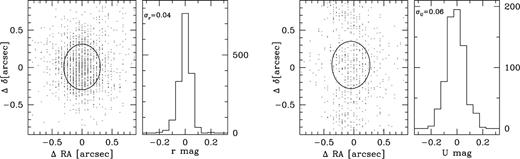
Astrometric and magnitude scatter in the r and U bands for objects in overlapping regions. The circle denotes the astrometric accuracy  .
.
The photometric calibration was performed using Landolt (1992) standard stars. We did not have sufficient standard stars on all the chips to solve for the extinction coefficients so we set the extinction coefficients to constant values. We used average extinction coefficients at the effective wavelengths of the filter+CCD system, as listed in Table 2, to derive the colour terms and zero points. The zero points are listed in Table 3. The colour terms were found to be very small (∼0.01) and are neglected. Because Coma lies close to the galactic pole, the extinction is insignificant for our purposes (0.043, 0.034 and 0.021mag in the U, B and r bands, respectively). Hence, we did not apply extinction corrections.
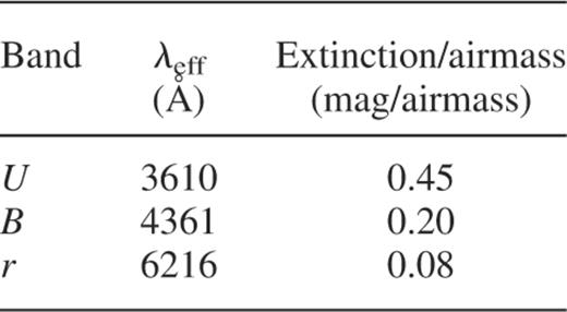
Average extinction coefficients for La Palma.
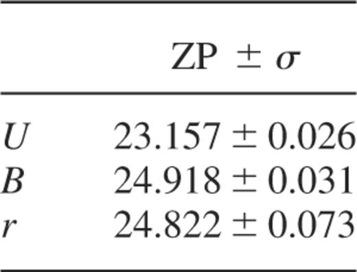
Zero points (ZP) of chip 4 for night 1.
Object catalogues
The data volume is considerable and requires a fully automated pipeline for data handling. After the standard reduction steps, the processed images were presented to software implemented at the Leiden Data Analysis Center (LDAC) for pipeline processing of overlapping images (Deul 1998). The processing software is a series of programmes that, when run in a chain, derive source parameters for any given set of input frames of a given passband. Only the first step is an actual data reduction task in that it reduces the information to be processed from image data to catalogue data (an object list). All but the last of the following pipeline routines add information to the catalogue(s) increasing its size and information content. The final step merges the catalogues to create a multicolour object catalogue with astronomically meaningful source information. The pipeline processing is performed on the full data set. Along the way we must decide on values for various parameters. We describe the pipeline steps in more detail below.
Detection of objects
We used SExtractor to automatically detect objects on each chip individually. The complete analysis of an image is achieved in six steps. First, a model of the sky background is built and parameters describing the global statistics are estimated. Then the image is background subtracted, filtered and thresholded. Detections are then deblended, cleaned, photometered, classified and written to the final catalogue. For specific details of each of these steps the reader is referred to Bertin & Arnouts (1996) or the SExtractor user's guide.
Objects were identified as the peaks in the (background subtracted) convolved images that were higher than a given threshold above the local background. We used most of the standard SExtractor settings except for the memory parameters which had to be increased in order to detect the large cD galaxies successfully. The seeing parameter had to be adjusted for each image individually for a good star/galaxy separation. For all objects positions, magnitudes, basic shape parameters and star/galaxy (S/G) classifiers were determined and written to a catalogue. SExtractor produced a catalogue for each image which was subsequently converted to a format suitable for pipeline reduction. As a first pipeline processing step, all information of the individual image source extractions plus all original fits image header information is combined into one single output catalogue per band.
Astrometry
Astrometric calibration was performed by pairing the input position catalogue (USNO A2) with the extracted object information. For multiple band processing intercolour pairing is done first and between frames in overlap, overlap pairing is performed as well. The derived astrometric solution is then applied to all the objects in the set of frames. Sky coordinates (RA and Dec.), as well as corrected geometric parameters are calculated. The final precision of this calibration depends on the accuracy of the source extractions, input catalogue accuracies and the correctness of the functional description of the distortions. We find  as shown in the left hand panels of Fig. 3.
Final object catalogue
The final step in creating a catalogue containing useful multicolour astronomical data is to merge all catalogues to get one source per position on the sky. All information referring to the same astronomical object is gathered and merged. Position information is a weighted mean of all the detections, where the weighting is based on the detection signal to noise ratio and environment conditions. Details of the merging are configurable. When the brightness contrast between overlapping galaxies is too low, the software is not able to deblend them correctly, resulting in an erroneous catalogue entry. On the other hand, setting the deblend contrast parameter too low causes SExtractor to consider bright star forming regions in a galaxy as separate objects. Then, there is the possibility that deblended objects are merged by the pipeline software when it is creating the final object catalogue. This can happen in cases where objects are small compared to the errors in position and shape parameters. We carefully inspected dense regions in our mosaic and conclude that erroneous catalogue entries are rare and consequently do not affect our results.
Star/galaxy separation was performed based on SExtractor's stellarity index. For bright objects stars and galaxies are easily separated, but towards fainter magnitudes and for bad seeing the division is not so clear. For most purposes we consider the objects with an S/G classifier value smaller than 0.8 in the r band (best seeing) to be galaxies. Bright (saturated) stars tend to have an S/G classifier smaller than this. We filtered these out by demanding an S/G classifier <0.1 for the brightest magnitudes. We visually inspected all bright objects to conclude that there is no contamination by stars up to at least  . Beyond
  we probably still have a fraction of stars in the sample, but for most purposes it is better to be contaminated by a (small) fraction of stars than to reject compact galaxies. Histograms of the catalogue's raw number counts are shown in the panels of Fig. 4. Throughout this paper we use SExtractor's mag_best as magnitude estimator. The final mosaic, composed of all pointings observed in the B and r bands, is shown in Fig. 5.
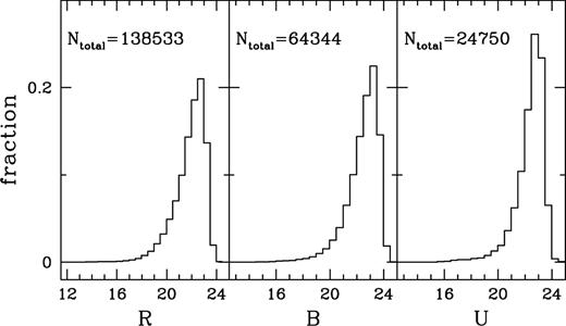
Histograms of the normalized raw r, B and U band number counts. Ntotal gives the total number of catalogue entries for each passband.
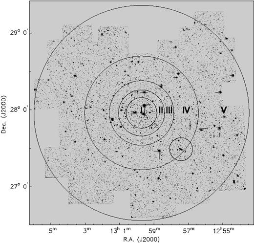
Overview of the total area covered in the B and r band with annuli overlaid. Radii are: I:  , II:
, II:  , III:
  , IV:
, IV:  and V:
  degrees
  at Coma distance). The circular area centred on NGC 4839 has a radius of 0.15°.
Control fields
For a survey as large and deep as ours, foreground/background subtraction can only be treated statistically, because only the brightest galaxies have measured redshifts. The main source of uncertainty in the determination of LFs comes from number statistics and background variance. Usually, flanking fields are used to get an estimate of the foreground/background correction and its variance. We expect that over the large area of the WFC the effects of cosmic variance are not important.
For the U band we have used  observations of an empty field located at
  ,
,  spanning ∼980arcmin2. For both the B and r bands we have made use of the Wide Field Survey (WFS) data archive to get images of random fields. The B band control images are eight 600s exposures, spanning ∼2000arcmin2 and centred at
  ,
,  and
and  ,
,  . The r band control images are four 600s exposures, spanning ∼1000arcmin2 centered at
  ,
,  . For the B and r band control fields we rely on the (photometric) reduction of the four chips by the WFS team.
All control images were pipeline reduced to give control catalogues which were filtered with the same criteria as the Coma fields. We applied relative extinction corrections (Schlegel, Finkbeiner & Davis 1998) to bring the extinction in the control fields into agreement with the Coma extinction, not zero extinction.
Completeness
The histograms shown in Fig. 4 suggest that the limiting magnitude is ∼22.5mag for all bands. However, because of the less than perfect conditions in the last two nights this limit does not apply to the total observed area. To have uniform completeness for the total mosaic we compute LFs up to  . The positions of these objects, relative to the cluster centre, are plotted in Fig. 6. The cluster is visible as a density enhancement on top of a uniform background. We have only considered clean detections (with good extraction flags) with more than five connected pixels above the background threshold.
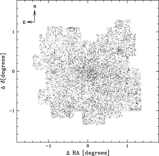
Distribution of objects with  . Coordinates are given relative to
  .
.
Detection limits in general depend on the interplay between scalelength/effective radius, magnitude and inclination, i.e. surface brightness. Edge on galaxies of a certain magnitude are easier to detect than their face on counterparts. Deep surveys have shown the existence of galaxies with surface brightnesses fainter than the night sky. These low surface brightness (LSB) galaxies are more likely to be missed at a given magnitude and inclination than their high surface brightness counterparts. Most of the LSB galaxies investigated in any detail are either late type and disc dominated (de Blok, van der Hulst & Bothun 1995; McGaugh & Bothun 1994), or giant, Malin 1 like galaxies (Sprayberry et al. 1995; Pickering et al. 1997).
In order to estimate these effects we followed two approaches. First we generated an r band luminosity–surface brightness plot for all objects (mostly galaxies) in our catalogue. The data in our catalogue do not contain estimates of the central surface brightnesses, but we can compute mean surface brightnesses for all objects based on total flux and area above the analysis threshold. In Fig. 7 we show the resulting luminosity–surface brightness plot along with the relevant magnitude and surface brightness selection boundaries we used. The dashed lines represent the luminosity–surface brightness relations for objects with the minimum detectable size (the seeing disc). We show minimum size detection lines for a seeing of 1.5arcsec and 1arcsec, from left to right, and it can be seen that occasionally the seeing drops even below 1arcsec. The mean isophotal limits for the U and B bands are 25.10 and 25.42magarcsec−2, respectively. From this figure it is evident that we are not likely to miss galaxies as a result of their low surface brightness. Secondly we generated artificial elliptical galaxies with de Vaucouleurs' law (de Vaucouleurs 1948) light profiles and spiral galaxies with exponential light profiles. We then added these galaxies into empty regions of our Coma images and verified whether SExtractor could recover these using the same selection criteria as for Coma fields. From our simulations we estimate that we are able to detect ellipticals with effective radii 
 or
or  down to ∼19.5, ∼19.5 and ∼19mag in the U, B and r band, respectively. Furthermore, we are able to detect dwarf galaxies modelled as exponential discs with
  down to ∼19.5, ∼20 and ∼20mag or
  , 24.3 and 24.3magarcsec−2 in the U, B and r band respectively. At the distance of Coma,
  corresponds to
  . Disc dominated LSB galaxies typically have
  and
and  . Assuming typical colours as in the de Blok et al. (1995) sample, this corresponds to
  and
and  . Our simulations show that such LSB galaxies are within our detection limits.
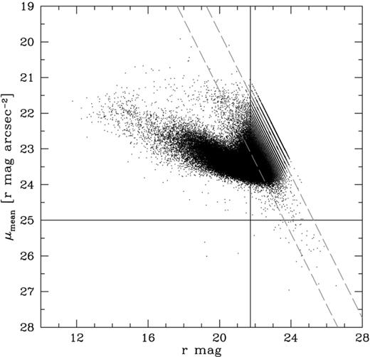
Luminosity versus mean surface brightness plot. The selection boundaries are indicated by the solid lines. The dashed lines represent the minimum size detection lines for a seeing of 1.5arcsec and 1arcsec (from left to right).
To illustrate the data quality we show examples of galaxies in Fig. 8. These have been drawn from our catalogue for magnitude bins  to −13 in steps of one magnitude, two examples per bin.
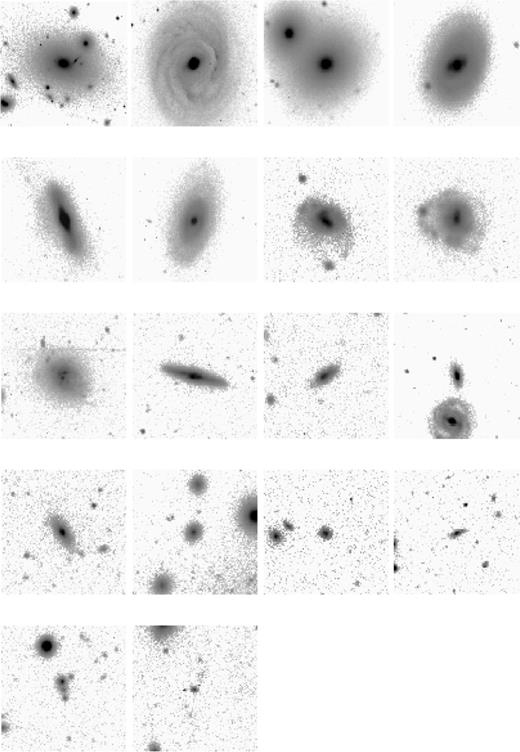
Examples of galaxies drawn from our catalogue for magnitude bins  to −13 in steps of one magnitude, two examples per bin.
Total luminosity functions
We constructed foreground/background corrected LFs by subtracting counts in the control catalogues from the Coma counts. From Fig. 4 it is obvious that the number of foreground/background counts is a strongly varying function of magnitude. Especially the faintest points of the LFs are largely influenced by an inaccurate determination of the amount of contaminating galaxies. We used very large control fields, and large bin widths compared to the photometric uncertainties. Therefore, effects caused by errors in the determination of foreground/background counts will be suppressed. Furthermore, we carefully calculated effective areas for all control fields and the Coma mosaic by counting unblotted pixels on each frame. Pixels which reduced the area for object detection, e.g. dead columns, saturated stars, etc., were blotted prior to the pixel counting. The total cluster counts and the field counts estimates are listed in Table 4.
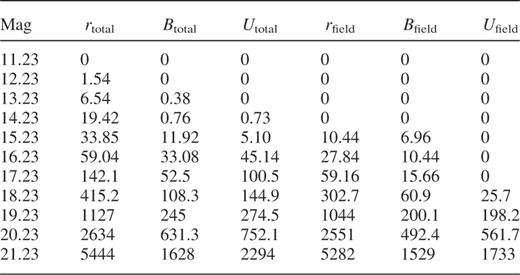
Total cluster counts and field counts estimates per deg2.
In Fig. 9 the LFs for the complete data set are shown. Solid lines represent best fitting Schechter functions with parameters as listed in Table 5. The faint end slopes increase towards shorter wavelengths. The best fitting Schechter functions are rather poor representations of the data for all bands, with several points lying more than 1σ away from the best fitting values. The χ2 statistic confirms the eye's impression that the LFs for the complete data set cannot be represented by single Schechter functions. These are the first accurate determinations of LFs for such large areas of a cluster. Furthermore, to our knowledge the U band LFs presented here are the first ever published for the Coma cluster.
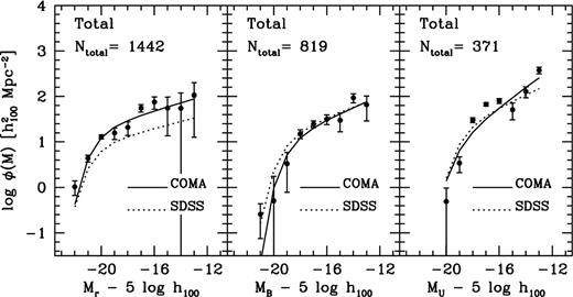
LFs for the total area observed. The solid lines represent best fitting Schechter functions with parameters as given in Table 5. The dashed lines correspond to the Sloan Digital Sky Survey field LFs. For clarity the SDSS LFs were renormalized by adding 2.8 to logφ(M) in all bands. Ntotal gives the estimated number of Coma galaxies up to −15.2.
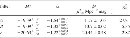
Best fitting Schechter parameters for the luminosity functions of the complete sample.
Dependence of luminosity functions on radial distance from the cluster centre
In order to study the dependence of the LF on radial distance from the cluster centre we defined five areas as annuli with varying widths and radii projected on the cluster centre, as shown in Fig. 5. For each of these areas we carefully determined the effective area for galaxy detection and constructed the corresponding LFs. The contamination by foreground/background galaxies becomes severe towards the outskirts of the cluster. Their numbers become equal to or greater than the Coma counts at  ,
,  and
and  in annulus I, III and IV, respectively.
We arbitrarily defined the core of the Coma cluster as the area with 
 (area I). This is comparable in size to the total observed areas in previous studies. In Fig. 10 we show the central LFs with best fitting Schechter functions overplotted as solid lines. The insets show the 68, 95 and 99 per cent confidence levels for the M* and α parameters that result from the fit to the binned data. The best fitting parameters are listed in Table 6. The bright end of the B band central LF is not adequately represented by the Schechter function. The faint end, however, is well represented by the Schechter fit. We do not confirm the dip, located at
  , reported by Biviano et al. (1995). We stress that our LF has been determined with completely different data and methods, complicating any direct comparison of results. Their estimate of the faint end slope
  is, however, in agreement with our result. Comparison of our B band LF with the typical richness class 2 composite cluster LF (Trentham 1998b) shows that the faint ends are consistent up to the completeness limit. Beyond the completeness limit the composite LF rises more steeply than the LF we have derived. Our value of the faint end slope of the central r band LF is in agreement with Lugger (1989),
 , but somewhat shallower than the slopes derived for Coma by e.g. Bernstein et al. (1995), López Cruz et al. (1997) and Secker, Harris & Plummer (1997) who all find
  . We stress that a direct comparison is hampered by the fact that these authors use different areas or composite LFs. To demonstrate more clearly that the LF is mainly shaped by the area we extracted Trentham's (1998a) area and constructed B and r band LFs. In Fig. 11 we compare the results of both determinations of the LFs. Up to the completeness limits the LFs are very similar showing that not the methodology employed, but the area chosen has the most crucial effect on the shape of the LF.
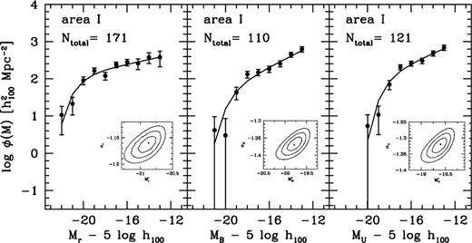
LFs for area I. Solid lines represent the best fitting Schechter functions with parameters as listed in Table 6. The insets show the 1, 2 and 3σ contour levels of the best fitting Schechter function parameters. Ntotal gives the estimated number of Coma galaxies up to −15.2.
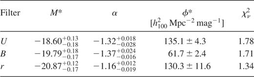
Schechter parameters for the central luminosity functions.
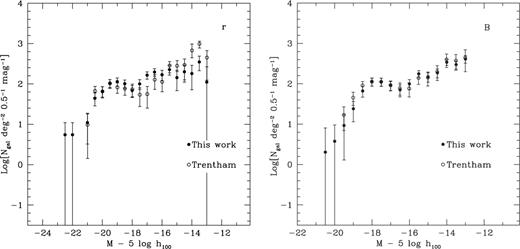
Comparison of our data to those of Trentham (1998a), restricting our data to the same area covered by the Trentham (1998a) survey. There is very good agreement between the two independent determinations of the Coma LF in this small region.
In general, a single Schechter function is a reasonable representation of all the central LFs, with two points lying 1σ or more from the best fitting value for all bands. It is expected from LF studies of composite dense and loose clusters and of single rich and poor clusters that the LF shape depends on environment. Below, we study the change in the shape of the LF as function of position in the cluster. We will examine whether differences can be attributed to effects of the local environment.
In the panels of Fig. 12 the LFs corresponding to the annuli II to V of Fig. 5 are shown for all bands. It is clear that these LFs are not simply scaled versions of the central LFs.
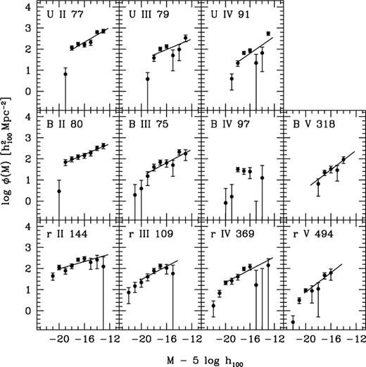
LFs for the annuli of Fig. 5. In the top of each figure we indicate: filter, annulus number and estimated number of Coma galaxies up to −15.2. The lines represent the fits to the faint ends.
The U band LFs are sensitive to star forming galaxies, and are therefore a poor indicator of the underlying mass distribution. They show significant curvature and at some radii dips, as reported for other bands (e.g. Biviano et al. 1995; Andreon & Pello 1999). Because of these dips, these LFs cannot be adequately fitted by single Schechter functions.
The B band LF of annulus II still resembles the central LF, but in annuli III and IV the faint end behaves differently. Even further out, in annulus V, the galaxies with  or brighter become very rare and the faint end seems to steepen again, but only marginally.
The r band LF of annulus II is relatively flat. At larger radial distances from the cluster centre the LFs become much steeper.
We quantified these trends as follows. We fitted a power law function (b 10aM) to the faint ends of the LFs in order to study their dependence on radial distance from the cluster centre. The LFs were fitted for  ,
,  and
and  , respectively. In Fig. 13 we plot the power law slopes as function of cluster radius. We omitted the slope of the B band LF for area IV: the value of the slope is extremely sensitive to the fitting region, and hence not well constrained. In general, the faint end slopes become steeper towards larger cluster radii.
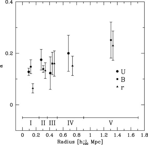
Power law slopes a as function of cluster radius. The faint ends of the LFs become somewhat steeper towards the cluster outskirts.
Comparison with field luminosity functions
In the field, the galaxy density is orders of magnitudes lower than in the cores of clusters like Coma. Galaxies in a dense cluster environment are likely to follow different evolutionary paths than galaxies in low density fields. It is therefore interesting to investigate whether this is reflected in their LF shapes. LFs of the field population have recently been measured by a number of surveys (e.g. Loveday et al. 1992; Lin et al. 1996, 1997, 1999; Geller et al. 1997; Marzke et al. 1998). Despite the large samples that were used to measure the LFs, controversy remains about the shape. One of the largest local redshift samples of galaxies selected from CCD images is provided by the Sloan Digital Sky Survey (SDSS) (Blanton et al. 2001). The SDSS survey has multicolour u′, g′, r′, i′, z′ photometry, whereas most of the older surveys measure LFs only for the B and R bands. We transformed the SDSS LFs into our photometric system using the transformations given in Fukugita et al. (1996). Similarly, values for the slopes in U, B, and r were obtained by interpolating between the nearest SDSS filters. The resulting SDSS LFs are shown in Fig. 9 as dashed lines. For clarity the LFs were renormalized by adding 2.8 to logφ(M) in all bands. The faint end slopes of the field LFs increase towards shorter wavelengths, although less significantly than in Coma. The faint end slopes of the r and B band LFs of field and Coma galaxies are very similar. Interestingly, the faint end of the Coma U band LF appears to be steeper than that of the field LF. This may indicate that dwarf galaxies at  in Coma have similar colours to dwarf galaxies in the field.
Galaxy distribution
The best indicator of the underlying mass distribution in our data set is the r band, because it is least influenced by episodic star formation. We use this band to investigate the projected galaxy density distributions. Following Driver, Couch & Phillipps (1998) we separate our sample into giant and dwarf galaxies. We define giant galaxies as objects with  and dwarf galaxies as objects with
  . In Fig. 14 we plot the projected distributions of these two types on the sky. In panels (a) and (b) of Fig. 15 we plot their foreground/background corrected projected densities and in panel (c) we plot their ratio as function of distance from the cluster centre. In panels (a) and (b) we also show isothermal profiles for comparison. The giant galaxies have a relatively small, sharply defined, area of high overdensity limited to the central cluster area. At a distance of
  from the cluster centre their density abruptly drops by ∼70 per cent and then decreases continuously. At distances from the cluster centre larger than
  the dwarf to giant ratio (D/G) could become somewhat larger than in the core of the cluster, but this is not significant given the large uncertainties.
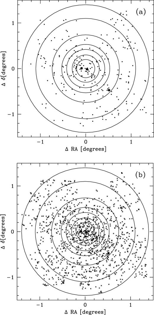
(a) Filled hexagons represent galaxies with  (giants). The three large hexagons represent NGC 4889, 4874 and 4839. (b) Crosses represent galaxies with
  (dwarfs). Overplotted are annuli with radii:
  ,
,  ,
,  ,
,  ,
,  ,
,  and
and  degrees
  at Coma distance).
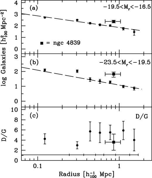
(a) The number density of dwarf galaxies as function of distance from the cluster centre. (b) The number density of giant galaxies as function of distance from the cluster centre. (c) The dwarf to giant ratio (D/G) as function of distance from the cluster centre. The NGC 4839 group is indicated by a square. Dashed lines correspond to isothermal profiles. Horizontal error bars indicate bin widths.
NGC 439 group
It has long been known that a secondary concentration of galaxies exists at ∼40arcmin south west of the cluster centre (e.g. Wolf 1901). This is the group associated with the cD galaxy NGC 4839. The presence of this group is clearly visible in Fig. 15: the density of the group lies well above the average density at that cluster radius and is comparable to the central densities. We used a circular area of 255arcmin2 centered on NGC 4839 (Fig. 5) to determine LFs. The LFs, shown in Fig. 16, are found to have different shapes than the central LFs (solid lines). Mobasher & Trentham (1998) have derived a K band LF for the field around NGC 4839. However, because of a small field size (9.9arcmin2) and large uncertainties in background subtraction, their LF is essentially unconstrained. Lobo et al. (1997) have derived a V band LF with a faint end slope comparable to their central LF, using an area of 117arcmin2. We find a B band LF which is much shallower than the central LF. The faint end of the U band LF is also flatter, except for the last point. In the r band we have a lack of galaxies fainter than  , but the faint end slope is comparable to the slope of the central LF.
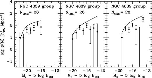
LFs for the area around NGC 4839. The best fitting Schechter functions of the central luminosity functions are overplotted to emphasize shape differences.
Discussion
In this paper we have used a statistical method to determine in U, B and r the LF of the galaxies in the Coma cluster and the dependence of the LF on projected distance from the cluster centre. We did find changes in shape as a function of radius indicating changes in the galaxy population in the cluster. At the same time this implies that comparison with other work is difficult as the LF shape depends critically on the area chosen for study. The changes in the LF shapes are very probably related to the local environment. We will accordingly discuss this possibility in more detail here.
The α parameter of the Schechter function effectively measures the faint end slope of the luminosity distribution and characterizes the intermediate and dwarf galaxy populations. A flat faint end slope implies a lack of these low luminosity galaxies. López Cruz et al. (1997) observe the trend that steep faint end slopes are detected in poorer clusters and the flatter slopes are, on average, found in richer clusters. This suggests that environmental properties could dictate the faint galaxy population. In a scenario in which mergers, interactions, tidal stripping, destruction of dwarfs, infall etc. play a role we expect to see a lack of faint galaxies towards the regions of higher galaxy density. This then should be reflected in a flattening of the low luminosity end of the LF. We do observe this effect; e.g. the slope of the faint end of the U band LF decreases from  at ∼
at ∼ to
to  in the centre. In terms of the slope of the Schechter function these values correspond to
  and
and  . The effect is also present in the B and r band LFs, and measured out to a larger radius of
  .
.
When comparing the faint end slopes of the Coma LFs with those from the SDSS, the most striking result is that the r and B band LFs are very similar. This is remarkable given the differences in environment and galaxy populations. However, the U band slopes of Coma are steeper than in the field, so apparently there is a relation between the relative increase in low luminosity systems in Coma and the colour of the band. A possible interpretation is that the (infalling?) dwarf galaxies in the outer parts of Coma are undergoing bursts of star formation triggered by interactions with neighbour galaxies and/or the intracluster medium. As a result the galaxies brighten, preferentially in the U band, causing a steepening of the faint end slopes of the LFs. If correct, this is a clear sign that the Coma cluster is not a relaxed system, but that, especially in its periphery, the cluster is still forming and inducing strong evolution to the galaxy population. The flattening of all Coma LFs towards the cluster centre hints that there the galaxies have already lost most of their gas and enhanced star formation has long ceased.
The group around NGC 4839 has been subject of debate in the literature, because it is not clear whether it is falling into the cluster for the first time or has already made one pass through (for scenarios see e.g. Colless & Dunn 1996; White, Briel & Henry 1993; Burns et al. 1994). Bravo Alfaro et al. (2000) have done Hi imaging of the Coma cluster and the NGC 4839 group. From the non detections in the close vicinity of NGC 4839 and the presence of several starburts and post starbust galaxies with very low Hi content in that zone they conclude that it passed at least once through the core. The LF of the field around NGC 4839 has a different faint end slope than the central LFs which could be related to the dynamical history of this group. The observed shape differences could be explained if during the passage a large fraction of the dwarf galaxies has been stripped from the group and redistributed throughout the cluster potential.
To explain the dependence of the shape of the LF on projected distance from the cluster centre we would need much more information. Knowledge of the galaxy morphologies, redshifts, the morphology density relation (Dressler 1980; Whitmore, Gilmore & Jones 1983), the type dependent LFs, Hi observations etc. are necessary to derive a complete scenario in which mergers, tidal stripping, infall etc. play a role. For instance, the observed dips and increasing faint end slopes could be the combined result of the morphological composition of Coma together with the shapes of the type dependent LFs.
Summary and conclusions
We have presented the first results of a wide field photometric survey of the Coma cluster in the U, B and r bands. The derivation of the source catalogue, along with the steps concerning the pipeline reduction, have been discussed. Our high quality data provides a valuable low z comparison sample for studies of galaxy morphology, colour and luminosity at higher z.
In this paper we have used the data to study the dependence of the galaxy LF on passband and projected distance from the cluster centre. The LFs of the complete data set cannot be represented by single Schechter functions. The central U, B and r band LFs can be represented by Schechter functions with parameters as listed in Table 6. The expectation that the shape of the LF depends on environment is confirmed. The LFs as a function of distance from the cluster centre have (very) different shapes than the central LFs and, therefore, no universal general LF exists. The faint ends of the LFs become steeper towards the outskirts of the cluster. A steepening of the faint ends of the LFs towards less dense regions clearly supports the existence of environmental effects. The difference in faint end slopes of the overall LFs and those of the field is colour dependent (strongest in U) and can be attributed to enhanced star formation in the dwarf galaxy population in the outer parts of Coma, where evolution apparently is still very strong. The LFs of the field around NGC 4839 support the idea that this group has passed through the cluster centre at least once.
We are in the process of creating a catalogue of all the spectroscopically confirmed cluster members. This will enable us to revise the Coma LFs and to check the quality of the statistical method to determine LFs. We have also obtained Westerbork Synthesis Radio Telescope (WSRT) Hi mosaic data covering a total area of  in order to study the Hi properties as function of environment and assess the importance of merging and stripping. Combined with our optical data set this will greatly enhance the ability to study the structure and dynamics of Coma, using a data set that is unrivalled by what is available for any other cluster.
Acknowledgments
This paper is based on observations made with the Isaac Newton Telescope, operated on the island of La Palma by the Isaac Newton Group in the Spanish Observatorio del Roque de los Muchachos of the Instituto de Astrofisica de Canarias. We thank the referee for detailed and constructive comments. Part of the data was made publically available through the Isaac Newton Groups' Wide Field Camera Survey Programme. PGvD acknowledges support by NASA through Hubble Fellowship grant HF 01126.01 99A awarded by the Space Telescope Science Institute, which is operated by the Association of Universities for Research in Astronomy, Inc., for NASA under contract NAS 5 26555.
References
Author notes
Hubble Fellow.
