


Abstract
We study the variation of the frequency splitting coefficients describing the solar asphericity in both GONG and MDI data, and use these data to investigate temporal sound-speed variations as a function of both depth and latitude during the period 1995–2000 and a little beyond. The temporal variations in even splitting coefficients are found to be correlated to the corresponding component of magnetic flux at the solar surface. We confirm that the sound-speed variations associated with the surface magnetic field are superficial. Temporally averaged results show a significant excess in sound speed around  and latitude of 60°.
1 Introduction
Helioseismology – the study of acoustic oscillations in the Sun – allows us to probe the solar interior structure and rotation in two dimensions, depth and latitude, by taking advantage of the different spatial distribution of the various modes. Recently, two projects – the Global Oscillation Network Group (GONG) and the Solar Oscillations Investigation (SOI) using the Michelson Doppler Imager (MDI) instrument aboard the SOHO spacecraft – have provided nearly 5 yr of continuous helioseismic data, allowing the rise of the current solar cycle to be followed in unprecedented detail.
Two-dimensional inversions for the rotation profile have been widely studied. Inversions for the structural parameters (for example, sound speed and density) are more commonly carried out in one dimension only. However, it is possible to access two-dimensional information on these parameters also, using the so-called ‘even a coefficients’; results of early attempts can be found in Gough et al. (1996). In the light of recent work by Antia & Basu (2000), Howe, Komm & Hill (2000a), Howe et al. (2000b), and Toomre et al. (2000), suggesting that the torsional oscillation pattern seen at the surface penetrates substantially into the convection zone, it is of interest to see whether the structural changes also penetrate deeper than has previously been thought. In the work presented here we examine changes in helioseismic determinations of the solar asphericity as the solar cycle progresses.
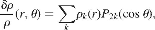
The modes are described by the radial order n, related to the number of nodes in the radial direction, and the degree l and azimuthal order m which characterize the spherical harmonic defining the horizontal structure of the mode. Rotation and asphericity lift the degeneracy between the  modes of different m making up an (n, l, m) multiplet, resulting in frequency splitting. The frequencies νnlm of the modes within a multiplet can be expressed as an expansion in orthogonal polynomials, for example
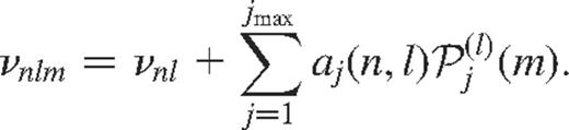
Earlier (e.g. Duvall, Harvey & Pomerantz 1986) Legendre polynomials were commonly used, whereas more recent work often uses the Ritzwoller–Lavely formulation of the Clebsch–Gordan expansion, where the basis functions are polynomials related to the Clebsch–Gordan coefficients (Ritzwoller & Lavely 1991)  by
by
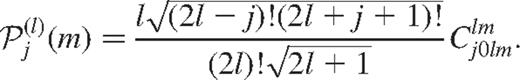
In either case, the coefficients aj are referred to as a coefficients. The odd-order coefficients, a1, a3, …, are used to determine the rate of rotation inside the Sun, and reflect the advective, latitudinally symmetric part of the perturbations caused by rotation. The even coefficients, which are much smaller, are sensitive to second-order contributions from rotation, any possible magnetic field and any possible departure of the solar structure from the spherically symmetric state. Since the rotation rate in the solar interior is determined by the odd-order coefficients, it can be used to calculate the second-order contribution of rotation to the even-order coefficients. Further, since the time variation in the rotation rate is small, being of the order of 0.5 per cent, the second-order contribution as a result of rotation may be expected to be essentially constant in time and hence any time variation in the even-order coefficients should be because of other sources, e.g. magnetic field or asphericity. Unfortunately, it is not possible to distinguish between these two possibilities using the even-order coefficients (Zweibel & Gough 1995).
It was well established during the previous solar cycle, that the even coefficients show temporal variations related to solar activity measures. The a2 and a4 coefficients of Duvall et al. (1986) were used by Gough & Thompson (1988) to infer the possibility of a shallow magnetic perturbation in the sound speed near the equator. Kuhn (1988a) also pointed out the relationship between a2 and a4 measurements from the Big Bear Solar Observatory (BBSO) and earlier data and the latitudinal variation of internal sound speed, noting the possibility of temporal variation as the known ‘hot bands’ associated with magnetic activity migrated during the solar cycle. The temporal variation of the a2 and a4 coefficients and its relation to changes in the latitudinal dependence of limb temperature measurements were further studied by Kuhn (1988b), Libbrecht (1989) and by Kuhn (1989), who predicted that the same relationship should extend to higher order coefficients. The inference from the inversions of the BBSO even a coefficient data carried out by Libbrecht & Woodard (1990) and Woodard & Libbrecht (1993) was that most of the variation in the even coefficients was localized close to the surface and at the active latitudes, with a near-polar variation anticorrelated to the global activity level. In the new cycle, we have data from GONG and MDI which allow us to study these trends in more detail. Howe, Komm & Hill (1999) have found linear relations between the even-order a coefficients and the Legendre decomposition components of the surface magnetic flux up to a8, and showed that these relations could be extended backwards in time to the BBSO data from the previous cycle. Dziembowski et al. (2000) found a good correlation between the even a coefficients derived from 12 72-d MDI data sets (1996 May 1–1998 May 31) and the corresponding even components of the Ca ii K data from BBSO up to a10.
It has been pointed out by Kuhn (1998) that the variations in mode frequency and even a coefficients are unlikely to be caused directly by the surface fields, as the fields required would be substantially stronger than those observed. However, this does not rule out the idea that the presence of magnetic fields affects the temperature. As pointed out by Dziembowski et al. (2000), the magnetic field might influence the thermal structure through the annihilation of the field (β effect) and indirectly through the perturbation of the convective transport (α effect) in addition to the direct mechanical effect of the Lorentz force. The good correlation between the magnetic activity indices and the variation in mean frequencies and even a coefficients would tend to suggest that the magnetic field probably plays some role in these temporal variations.
In the present work we use more extensive data sets from both GONG and MDI, extending the GONG analysis up to a14, and present the results of two-dimensional inversions for the sound speed. We effectively assume that the even-order a coefficients arise from aspherical sound-speed distribution, rather than being because of possible magnetic field effects.
2 Data
We have analysed 53 overlapping 108-d time series of GONG data covering the period from 1995 May 7 to 2000 October 6, centred on dates 1 36-d ‘GONG month’ apart. The data were analysed through the standard GONG pipeline (Hill et al. 1996), to find frequencies for each mode, and then a coefficients were derived by fitting to the frequencies in each (n,l) multiplet. A typical mode set from this process would consist of around 1400 multiplets with coefficients up to a15, for  the intersection of all the sets contains about 400 multiplets mostly with
  .
.
The MDI data consist of 23 non-overlapping time series covering the period from 1996 May 1 to 2001 April 4, although with some interruptions because of problems with the SOHO satellite. The data were analysed as described by Schou (1999). These sets contain coefficients, up to a36, for roughly 1800 multiplets with  . The substantial temporal overlap between the two sets allows useful cross-checking of results.
For the purpose of the inversions we have used only p-mode splittings for modes with frequencies between 1.5 and 3.5 mHz. Further, only coefficients up to a14 are used as the higher order coefficients do not appear to be significant. This gives us typically 8000 coefficients for MDI data sets and 6000 coefficients for the GONG data sets. Frequencies for f modes  are also available for the MDI data, and might provide additional information, but they have not been used in the current work.
3 Coefficient analysis
3.1 Method
Howe et al. (1999) considered the temporal variation of the GONG mean even a coefficients up to a8 and showed that they were strongly correlated with the corresponding components of the Legendre decomposition of the surface magnetic field. In the present work we extend this analysis, with some modifications, to coefficients up to a14 and to MDI as well as GONG data.
The latitudinal distribution of the surface magnetic flux can be expressed as a sum of Legendre polynomials in cos θ,
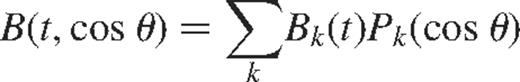
where Bk(t) are time varying coefficients. These coefficients can be compared with the corresponding frequency splitting coefficients. Global helioseismic measurements are sensitive only to the latitudinally symmetric part of any departures from spherical symmetry – that is, to the even components of the expansion.
For the purposes of the present work, we consider two weighting schemes. In the first, the splitting coefficients were weighted by Enl, where Enl is the mode inertia defined as in Howe et al. (1999) and references therein, normalized to set the value for the radial mode at 3 mHz to unity. In the second they were weighted by  , where Qlk is defined in equation (11) below, before averaging over all common multiplets. This removes the main l-dependent part of the coefficient variation, and also reduces the frequency dependent part. Thus, we define the quantities
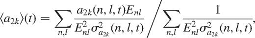
and
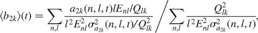
where t is the time and σak is the estimated uncertainty in the coefficient ak, and the sum is over the approximately 400 (n, l) multiplets that are common to all the mode sets.
We then express the variation of the 〈ak〉 and 〈bk〉 as a function of the Bk, for even k, as
and perform linear least-squares fits to obtain the gradient mk and intercept ck for each k. The intercept will contain a contribution from the invariant part of the coefficients which includes the second-order effect of rotation, as pointed out by Woodard (1989), Gough & Thompson (1990) and Dziembowski & Goode (1992).
3.2 Results
In Fig. 1 we show the variations of the mean coefficients  as a function of time, for the sets of modes common to all data sets. The correlation between the coefficients and the Legendre components of the surface flux persists up to a14 in both sets of data (Table 1). (The value of the correlation coefficient R required for the 0.1 per cent significance level is 0.45 for GONG and 0.68 for MDI.) There is a reasonably good agreement between GONG and MDI data for
  , but for a14 the agreement is less good. We suspect the difference may be because of the different analysis procedures used for calculating the splitting coefficients in the two data sets. In principle, B0 may be correlated to the temporal variations in the mean frequencies, but in practice, it is difficult to separate out the contributions to the mean frequency due to the magnetic field from those due to uncertainties in the spherically symmetric structure of the Sun. For this reason, we do not compare the component B0 in this work.
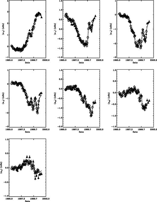
Temporal variation of the GONG (open circles) and MDI (filled triangles) mean even a coefficients. The quantity plotted is 〈ak〉, as defined in equation (4). The curves show the best-fitting values  for linear fits between the 〈a2k〉 coefficients and the corresponding B2k components of the Legendre decomposition of the magnetic flux, for GONG (solid) and MDI (dashed).
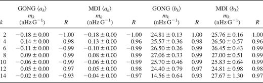
Gradients m and correlation coefficients R for fits between the weighted mean coefficients 〈ak〉, 〈bk〉 and the corresponding Legendre components Bk of the unsigned magnetic flux.
In Fig. 2 we show the coefficients  as a function of the corresponding components
  of the surface magnetic flux, for GONG and MDI, while the left portion of Table 1 gives the slopes mk and correlation coefficients for the fits between even a coefficients and their corresponding magnetic flux decomposition components. While alternate even coefficients
  appear to be anticorrelated with Bk, the other coefficients
  are correlated with Bk. There also appears to be a reduction in the magnitude of 〈ak〉 with k for
  , while the Bks do not show such a marked decrease. However, the 〈b2k〉 (Fig. 3, right side of Table 1) are all positively correlated with B2k with scaling constants that appear to be independent of k, except for the highest order coefficients where the GONG data show some reduction in sensitivity. In fact, most of the variation, including the sign changes, in the 〈ak〉 slopes up to
  can be explained by the corresponding variation in the angular integrals, Qlk.
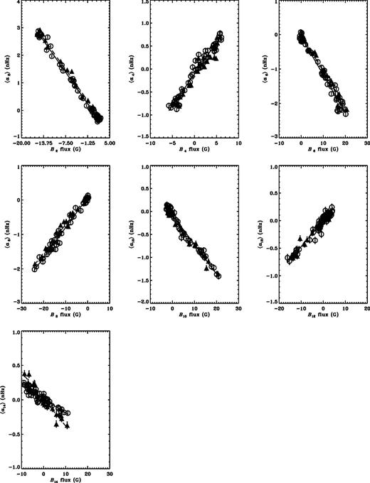
The relations between the GONG (open circles) and MDI (filled triangles) 〈ak〉 coefficients and the corresponding Bk components of the Legendre decomposition of the magnetic flux from the Kitt Peak synoptic maps. The lines show the best-fitting results for linear fits to the data, for GONG (solid) and MDI (dashed).
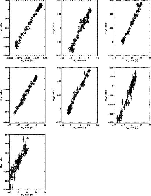
The relations between the GONG (open circles) and MDI (filled triangles) 〈bk〉 coefficients and the corresponding Bk components of the Legendre decomposition of the magnetic flux from the Kitt Peak synoptic maps. The lines show the best-fitting results for linear fits to the data, for GONG (solid) and MDI (dashed).
4 Asphericity inversions
4.1 Inversion techniques
In order to study the variation of asphericity with depth and latitude we apply an inversion technique to the even-order splitting coefficients. We use the variational principle to analyse the departures from a spherically symmetric solar model (e.g. Gough 1993), in order to study aspherical perturbations to the sound speed and density in the solar interior. For simplicity, we only consider axisymmetric perturbations (with the symmetry axis coinciding with the rotation axis) that are symmetric about the equator. In this case, using the variational principle, the difference in frequency between the Sun and a solar model for a mode of a given order, degree and azimuthal order (n, l, and m) can be written as:
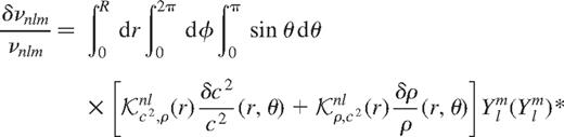
where r is the radius, θ is the colatitude,  is the relative frequency difference,
  and
and  are the kernels for spherically symmetric perturbations (Antia & Basu 1994), and
  are spherical harmonics denoting the angular dependence of the eigenfunctions for a spherically symmetric star. It is assumed that the
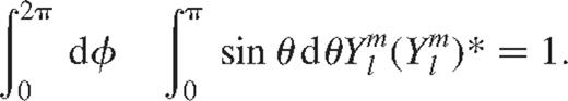
  are normalized such that
The perturbations  and
and  can be expanded in terms of even-order Legendre polynomials:

where ck(r) and ρk(r) are shorthand notations for  and
and  , respectively. The spherically symmetric component
  gives frequency differences that are independent of m and thus only contribute to the mean frequency of the (n, l) multiplet. Higher order terms give frequencies that are functions of m and thus contribute to the splitting coefficients.
The angular integrals in equation (7) can be evaluated to give
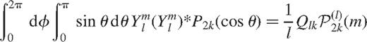
where Qlk depends only on l, and k and  are the orthogonal polynomials defined by equation (2). The extra factor of
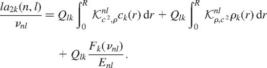
  ensures that Qlk approaches a constant value at large l. Thus with this choice of expansion (equation 2) the inversion problem is decomposed into independent inversions for each even splitting coefficient and ck(r), ρk(r) can be computed by inverting the splitting coefficient a2k. This would be similar to the 1.5 d inversion to determine the rotation rate (Ritzwoller & Lavely 1991), called so because a two-dimensional solution is obtained as a series of one-dimensional inversions.
In practice, we also need to account for the contribution to the frequency splittings that arises from uncertainties in the treatment of surface layers in the model. It is known that this contribution to frequency splittings should be a slowly varying function of frequency alone once it is corrected for differences in the mode mass of the modes; no degree dependence is expected to a first approximation. As in the case of inversions to determine the spherically symmetric structure of the Sun, the surface uncertainties are accounted for by assuming that these can be represented by a frequency dependent function F(ν). However, in this case we determine a different function Fk(ν) for each coefficient a2k and write the inversion problem as
equation (12) can be inverted using the usual inversion techniques to calculate ck(r), ρk(r) and Fk(ν). We use a regularized least-squares (RLS) technique for this purpose and expand the unknown functions ck(r), ρk(r), Fk(ν) in terms of cubic B-spline basis functions over knots, which are approximately uniformly spaced in acoustic depth (or frequency). First derivative smoothing is applied to constrain the error in the solution to remain small.
As in the case of inverting for rotation rate it is possible to apply a 2d inversion technique for asphericity, where the asphericity is not expanded in terms of Legendre polynomials, but instead one uses
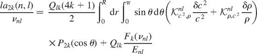
where  and
and  are now functions of (r, θ) and can be expanded in terms of a set of 2d basis functions for the RLS inversion. The knots are chosen to be uniformly spaced in acoustic depth and cos(θ) and we use the product of B-spline basis functions in r and cos(θ). Thus, for example, we can write
where bij are the coefficients of expansion and φi(r) are the B-spline basis functions over r and ψj(cos θ) are those over cos θ;nr and n are the number of basis functions in r and cos θ, respectively. The unknown functions  ,
,  and Fk(ν) are expanded in terms of basis functions and the coefficients of expansion are determined by solving one inversion problem involving all splitting coefficients. First derivative smoothing is applied for both r and cos θ. Thus, the coefficients of expansion are determined by minimizing
where λr and λ are the two regularization parameters controlling the smoothing and  and
and  are the 2d kernels, σnlk are the uncertainties in a2k(n, l). We have used 16 knots in r and 10 knots in cos θ to represent the asphericity.
4.2 Inversion results
In Fig. 4 we show the results of sound-speed inversions of GONG and MDI data at selected radii as a function of time and latitude. There is no signature of significant temporal evolution at these radii. Both sets of data show a persistent sound-speed excess at around 60° apparently extending well down into the convection zone, although this is more significant in the MDI than in the GONG data.
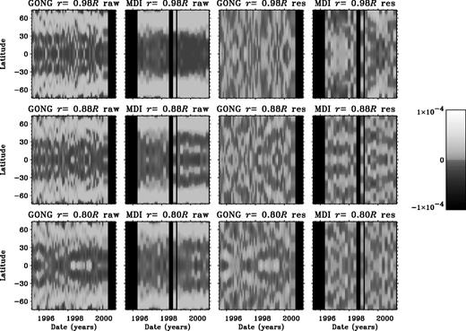
Grey-scale maps showing the results of sound-speed inversions of GONG (first and third columns) and MDI (second and fourth columns) data at radii 0.98R (top), 0.88R (centre) and 0.80R (bottom). Blank spaces represent periods where there are no data available. Columns 1 and 2 show the 1.5 d inversion results and columns 3 and 4 the 2d results.
The inversions show the deviation from a spherically symmetric model. It turns out that the temporal mean of these deviations is non-zero and has a dependence on depth and latitude, as illustrated in Fig. 5. However, it may be noted that the current data extend over only a small fraction of a magnetic cycle and the temporal mean over this limited period may not have much significance. The second-order contribution from rotation would also contribute to the temporal mean. There is some difference between the mean calculated from GONG and MDI data sets, which could be because of systematic differences between the two sets. In both cases there is a peak around depth of 0.08 R⊙ and the peak is more pronounced in MDI data.
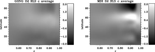
Grey-scale maps showing the mean results of sound-speed inversions of GONG (left) and MDI (right) data, multiplied by 104, as a function of latitude and radius.
The sound-speed variation after subtraction of the mean profile is shown in Fig. 6. No systematic structure is evident. Fig. 7 shows the variation of the sound-speed residuals from the 2d inversions of GONG and MDI data at selected (r, θ) points, illustrating the agreement between the two experiments. The residuals are obtained by subtracting the temporal mean from the results at each epoch. It is clear from these figures that there is no significant temporal variation in the asphericity at the depths we can resolve.

Grey-scale maps showing the results of sound-speed inversions of GONG (first and third columns) and MDI (second and fourth columns) data at radii 0.98R (top), 0.88R (centre) and 0.80R (bottom), after subtraction of the temporal mean. Blank spaces represent periods where there are no data available. Columns 1 and 2 show the 1.5 inversion results and columns 3 and 4 the 2d results.
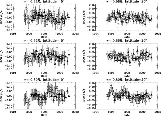
Variation of GONG (open) and MDI(filled) sound-speed residuals at radii 0.98R (top), 0.86R (middle), and 0.8R (bottom) for latitudes of 0° (left) and 20° (right.)
The strong variation in the even a coefficients is evidently not reflected in the inversion results. Instead, it has been absorbed in the surface terms. To illustrate this, we show in Fig. 8 the reconstruction of the surface term for a frequency of 2.5 mHz, with overlaid contours of the magnetic flux. As we would expect, since the dependence of the individual surface terms on frequency and on the magnetic field strength is largely independent of the order of the coefficient, this reconstruction matches the magnetic flux quite well. This finding is consistent with the results of Woodard & Libbrecht (1993), who carried out latitudinal inversions of the coefficients up to a12. They found that the sound speed showed a peak at the active latitudes, matching both magnetic and temperature behaviour, and also a decline at high latitudes with increasing solar activity which was better matched by the temperature than by the magnetic data. The surface terms from our inversion show a similar high-latitude behaviour, which does in fact correspond well to the high-latitude magnetic data; we attribute this to an improvement in the magnetic observations since 1992. Our inference that most of the solar-cycle variation in the sound speed is localized near the surface is also in agreement with the conclusions of Woodard & Libbrecht (1993).
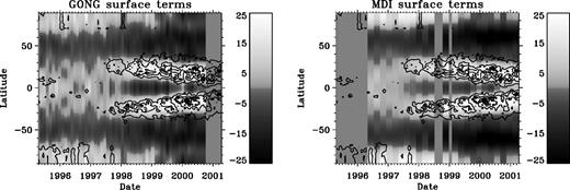
Grey-scale map showing the reconstruction of the latitudinal dependence of the surface term from GONG (left) and MDI (right), multiplied by 100. Overlaid contours show the Kitt Peak unsigned magnetic flux with the B0 term subtracted; contour spacing is 10 G.
5 Resolution issues
In order to test our inversion method and to see how well the inversions can resolve different features, we have conducted tests with artificial data. Since asphericity inversions do not include the spherically symmetric component corresponding to the mean frequencies,  integrated over a surface with constant r must vanish. This arises because the non-vanishing part of the integral can only contribute to the mean frequencies, which are not included. Furthermore, the even splitting coefficients are sensitive only to the north–south symmetric component of the asphericity. Thus it is necessary to choose artificial data which assume a profile that integrates to zero in latitude and which are symmetric about the equator. We have chosen a profile of the form
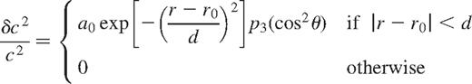
where r0 and d are constants which respectively, define the mean depth and half-width of the aspherical perturbation and p3(cos2θ) is a third-degree polynomial in cos2θ which integrates to zero. There is no special reason to choose a third-degree polynomial, except that with this choice one can get two bands of positive and negative asphericity in each hemisphere. The amplitude a0 of the signal is chosen to match the observed signal approximately.
Using the artificial profile for  with the peak located at different radii and with different widths, we construct a set of artificial data. These data include only those modes which are present in the observed data, and random errors with a Gaussian distribution with standard deviation equal to the estimated uncertainties in observed data are added to the calculated splittings. The amplitude a0 is chosen to be comparable to that obtained from real solar data. This process is followed for both GONG and MDI data sets. These artificial data were then inverted the way we would invert the real data and using the same choice for smoothing as is used for the real data. The inversion results can be compared with the actual profile used in constructing the artificial data.
The inversion results show that we are able to invert for the aspherical sound-speed difference in the outer layers of the Sun. Fig. 9 shows the inversion results for artificial data with the peak located at different depths. These results indicate that with the current data sets we cannot invert for any feature located below a radius of 0.8 R⊙. At smaller radii, e.g. 0.7 R⊙, although we get some result at the equator, the artificial profile is not reproduced properly at high latitudes. Similarly, the results become unreliable above 0.98 R⊙, mainly because of the lack of high-degree modes. The inversion results are reliable between depths of 0.02 and about 0.2 R⊙. As with all RLS inversions, there is some structure in the results away from the peak, but the structure is small and does not give rise to any major artefacts. The figures shown give us confidence in the results we obtain by inverting the real data.
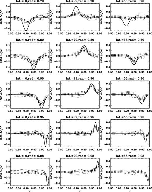
Artificial data inversion results for a variety of radial distances (from top to bottom,  , 0.8 R, 0.9 R, 0.95 R and 0.98 R) and latitudes (from left to right, latitude 0°, 30° and 56°), for GONG (dotted curves) and MDI (dashed curves.) The solid curves show the ‘true’ rate and the thinner dashed and dotted curves represent 1σ error bounds on the inversion results.
A similar exercise was also carried out for the inversions of density, but with an amplitude of artificial profile comparable to those in real data, it was not found to be feasible to reproduce the profile to any reasonable accuracy at all depths. Thus it appears that the aspherical component of density cannot be reliably determined from current data sets. Therefore, we do not show these results in the present work.
6 Discussion
We have studied the temporal variations in even a coefficients from GONG and MDI data during the period 1995–2001. The mean values of the even a coefficients (after scaling for mode mass and angular integrals) over all modes are found to be well correlated to the corresponding components of the observed magnetic flux at the solar surface. The slope of the best linear fit between the mean splitting coefficient and the corresponding Legendre component of the surface magnetic flux is found to be essentially independent of the order of the coefficient. Thus the latitudinal variation in the surface magnetic flux is correlated with that in asphericity as measured by the even a coefficients. Dziembowski et al. (2000) obtained similar results analysing 12 72-d MDI data sets (1996 May 1–1998 May 31). They found a good correlation between the even a coefficients (up to a10) and the corresponding even components of the Ca ii K data from BBSO.
In this work we have carried out two-dimensional inversions for sound speed using even a coefficients from GONG and MDI data sets covering the period from 1995 to early 2001, encompassing the rising phase of the current solar cycle. We find no significant temporal variation in the asphericity of sound speed over this period. Thus it appears that the temporal variations in even a coefficients arise from changes taking place in the surface layers. A similar conclusion has been obtained for the spherically symmetric component of sound speed and density (Basu & Antia 2000) as the changes in mean frequency also appear to be associated with surface effects.
For this work we have assumed that the even a coefficients arise from aspherical sound-speed distribution, but this is by no means obvious as these coefficients could also arise from a magnetic field since both sets of kernels are very similar in most parts of the Sun and cannot be easily distinguished (see, for example, fig. 10 in Dziembowski et al. 2000). In that case a magnetic field strength yielding  would be required, where vA is the Alfvén speed. Inside the convection zone one might not expect an ordered magnetic field over large length-scales as turbulence might be expected to randomize the magnetic field. Such a randomized magnetic field can also effectively change the wave propagation speed, giving a signal similar to that from an aspherical sound-speed distribution. It may not be possible to distinguish between these two effects from the even a coefficients. Kuhn (1998) has argued that the observed magnetic field at the solar surface is not sufficient to explain the magnitude of the even a coefficients. However, one can argue that the magnetic field increases significantly as one goes deeper in the near surface layers and this could explain the observed magnitudes of the splittings.
The aspherical component of the density cannot be reliably determined from the current data sets, but the magnitude is generally found to be smaller than that for the sound speed. If the aspherical perturbations were of thermal origin then one might have expected the density perturbations to be comparable to the sound-speed perturbations.
Although the temporal variation in asphericity in the solar interior is not significant, the mean asphericity is found to be significant and shows a peak around  which is very pronounced in the inversions of MDI data. This is deeper than the depth to which the surface shear layer in solar rotation rate extends (Schou et al. 1998) and is about the same as the penetration depth recently (Antia & Basu 2000; Howe et al. 2000) established for the torsional oscillation pattern. Antia, Chitre & Thompson (2000) attempted to detect a possible signature for magnetic field using the even a coefficients to find that the coefficients a2 and a4 have a residual after subtracting the contribution from rotation, which is peaked around
  , which is consistent with our results. Dziembowski et al. (2000) calculated inversions separately for temperature and magnetic field perturbations and detected a significant perturbation in the spherically symmetric part at a depth of
  with a maximum at about 45 Mm, which agrees with the depth at which we find the aspherical perturbation in the sound speed. They interpret this perturbation as being either because of a magnetic perturbation of about (60 kG)2 or because of a temperature perturbation of about
  which is of the same order as the result presented here. Gilman (2000) pointed out that a thermal driving mechanism for the observed meridional flow would require a temperature excess at the equator – the opposite of what we observe. Thus this finding poses yet another challenge for theoretical understanding of the dynamics of the convection zone.
Acknowledgments
This work utilizes data obtained by the GONG project, managed by the National Solar Observatory, which is operated by AURA, Inc. under a cooperative agreement with the National Science Foundation. The data were acquired by instruments operated by the BBSO, High Altitude Observatory, Learmonth Solar Observatory, Udaipur Solar Observatory, Instituto de Astrofísico de Canarias, and Cerro Tololo Interamerican Observatory. The SOI involving MDI is supported by NASA grant NAG 5-3077 to Stanford University. SOHO is a mission of international cooperation between ESA and NASA. RWK, and RH in part, were supported by NASA contract S-92698-F. NSO/Kitt Peak data used here are produced cooperatively by NSF/NOAO, NASA/GSFC, and NOAA/SEL.
References
