Planets in 47 Tuc

Abstract

1 Introduction

The search for extra-solar planets came to fruition in 1992 when Wolszczan & Frail (1992) discovered the first confirmed extra-solar planets orbiting the pulsar 1257+12. Since Wolszczan's discovery, conventional optical searches have found a number of extra-solar planets, biased towards the so-called ‘hot Jovians’, typified by 51 Peg (Mayor & Queloz 1995; Marcy & Butler 1996). The observing techniques, measurement of low-amplitude periodic Doppler shifts in the primary, bias such searches towards high-mass planets with short orbital periods. Recently, the nature of these systems, gaseous giant planets in short-period orbits, was confirmed by the observation of a transit in the HD 209 458 system (Charbonneau et al. 2000).

A second pulsar–planet system has also been observed. PSR B1620–26 in the globular cluster M4 is a binary pulsar with a low-mass white dwarf secondary in a ∼1 au near-circular orbit (Lyne et al. 1988). In 1993 Backer et al. discovered the presence of a second orbiting companion, conjectured to have a planet mass (Backer, Foster & Sallmen 1993; Sigurdsson 1993; Thorsett, Arzoumanian & Taylor 1993). Subsequent observations have confirmed the presence of a second companion around 1620–26. The second companion has substellar mass and it is nearly certain that the object is a planet (Thorsett et al. 1999). M4 is a modest, relatively low-metallicity cluster, and the most plausible formation scenario requires that the planet was exchanged into the pulsar system during an encounter with a main-sequence star in the cluster (Sigurdsson 1993, 1995; Joshi & Rasio 1997; Ford et al. 2000). The implication is that Jovian mass planets must exist around at least some of the main-sequence stars in relatively low-metallicity globular clusters. The progenitor system of the M4 planet must have had the planet in a wide orbit just before the exchange encounter (a » 1 au), in order for it to have been plausibly exchanged into the current configuration.

Recently, a Hubble Space Telescope project (GO-8267) carried out a transit search for ‘hot Jovians’ in the globular cluster 47 Tucanae. The observations involved the continuous monitoring of several tens of thousands of stars using WF/PC2 and STIS. The basic technique was to take short (few minute) exposures, primarily alternating I- and V-bands. A single field in the cluster, with the PC chip centred on the edge of the cluster core, was monitored continuously for over 8 d.

The search is sensitive to Jovian-sized planets with orbital periods ≲4 d, orbiting main-sequence stars in the cluster. A detection requires two observations of a dimming of a few millimagnitudes in both bands, lasting several hours (typical transit times-scales are 3 h). Only relative photometry is required, and about 34 000 stars were monitored simultaneously.

If the distribution of orbital parameters of Jovian planets in 47 Tuc is comparable to that in the stellar neighbourhood, for short orbital periods, then given a random orientation of orbital planes, the search should discover some 15–20 51 Peg-like planets.

Globular clusters are crowded environments. Binary systems undergo dynamical interactions with nearby stars, and close encounters can lead to large changes in orbital parameters, including the disruption of the system (Heggie 1975; Hut & Bahcall 1983). It is of interest to consider the probability of a planetary system surviving for a time comparable to the Hubble time in the inner regions of globular cluster, and the possible dynamical evolution of high-mass-ratio binaries in such environments. Considerable work has been done on this problem, including the pioneering analysis of Heggie (1975) and the numerical experiments of Hills (1975) and Hut & Bahcall (1983), and more recently simulations directed at specific problems in globular clusters (Davies 1995; Davies & Benz 1995; Sigurdsson & Phinney 1993, 1995). Relatively little work has been done on the problem of very high-mass-ratio systems appropriate to planetary encounters, Sigurdsson (1992) considered the basic problem, Laughlin & Adams (1998) calculated mean disruption rates for open clusters, and Bonnell & Kroupa (1998) looked at the issue in the context of planet formation. Hills (1984) considered close encounters between a star–planet system and an intruder star. Hills & Dissly (1989) extended this work to consider a range of impact velocities and intruder masses. For the M4 system, considerable effort has been made to simulate its possible dynamical history and the implications of the existence of such a system (Sigurdsson 1993, 1995; Joshi & Rasio 1997; Ford et al. 2000).

47 Tucanae is a massive and quite dense cluster. The central density is about 1.5 × 10⁵ pc⁻³ with a central velocity dispersion of ∼12 km s⁻¹. The core radius is about 0.5 pc and the half-mass radius about 3.9 pc (Djorgovski 1993; Howell, Guhathakurta & Gilliland 2000). At the half-mass radius the number density of stars is about a factor of ten lower than in the core.

2 Encounter time-scales

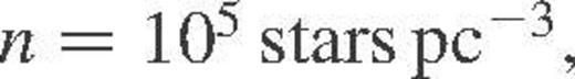
Encounters between two stars will be extremely rare in the low-density environment of the solar neighbourhood. However, in the cores of globular clusters number densities are sufficiently high (∼10⁵ stars pc⁻³ in some systems) that encounter time-scales can be comparable, or even less than, the age of the universe. In other words, a large fraction of the stars in these systems will have suffered from at least one close encounter or collision in their lifetime.

The cross-section for two stars, having a relative velocity at infinity of V_∞, to pass within a distance R_min is given by

(1)

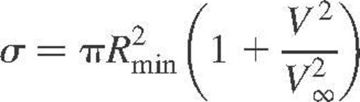
where V is the relative velocity of the two stars at closest approach in a parabolic encounter (i.e. . The second term arises from the attractive gravitational force, and is referred to as gravitational focusing. If V » V_∞, as will be the case in systems with low velocity dispersions, such as globular clusters, .

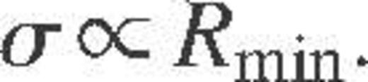One may estimate the time-scale for a given star to undergo an encounter, . For clusters with low velocity dispersions, we thus obtain

(2)

where n is the number density of single stars of mass M.

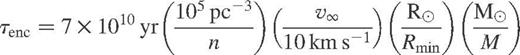
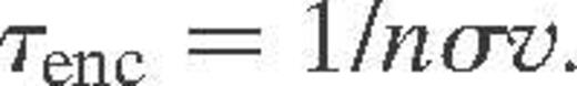
We may estimate the time-scale for an encounter between a star–planet system and a single star, in a similar manner where now R_min ≃ d,, where d is the semimajor axis of the planet's orbit. The encounter time-scale for such a system may therefore be relatively short as the semimajor axis can greatly exceed stellar radii. For example, a planetary system with (≡216 R_⊙), will have an encounter time-scale in the core of a dense globular cluster.

Encounters between single stars and binary systems will lead to the breakup of the binaries when the kinetic energy of the incoming star exceeds the binding energy of the binary. This will be the case when , where

(3)

where M₁ is the mass of the primary, M₂ is the mass of the secondary and M₃ is the mass of the incoming, single star. Binaries vulnerable to breakup are often referred to as being soft (Heggie 1975; Hut & Bahcall 1983). In the case of encounters between single stars and a star–planet system, the latter will be invariably soft as and M₃. We would therefore expect the planetary system to be broken up with some high probability, when an intruding star passed within a distance d of the planetary–system star (but see Sigurdsson 1993). In addition, more distant encounters may leave the planets in somewhat eccentric orbits, as will be discussed later. The importance of encounters between a planetary system and binaries is a function of the binary fraction within the cluster, which is not well known.

3 Numerical methods

For encounters involving a single intruding star, we used a code based on that discussed in Davies, Benz & Hills (1993). For encounters involving binaries (i.e. four objects), we used a code based on that discussed in Bacon, Sigurdsson & Davies (1996).

The initial conditions for the scatterings were set following the method of Hut & Bahcall (1983, see also Sigurdsson & Phinney 1993). With two binaries, we have additional parameters from the relative phase of the second binary, the orientation of the plane of the second binary and the second binary mass ratio, semi-major axis and eccentricity. We drew the binary parameters by Monte Carlo selection uniformly over the phase variables. The relative velocity at infinity of the centres of mass of the two binaries, v_∞ was chosen uniformly on the interval allowed. The initial binary eccentricities, e_1,2 were zero for all encounters, previous calculations indicate that the cross-sections of interest are not sensitive to the eccentricities of the binaries.

For encounters involving single stars, the equations of motion are rescaled using the Heggie (1972) quasi-regularization and are integrated using the variable-order, variable-stepsize Shampine–Gordon integrator (1975). For encounters involving binaries, a Bulirsch–Stoer variable step integrator with KS-chain regularization (Aarseth 1984; Mikkola 1983, 1984a,b) was used for integrating the motion of the particles.

4 Results

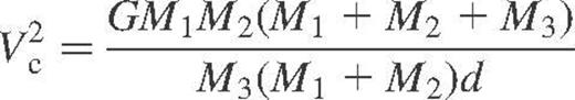
We considered encounters between a star–planet system and either a single star or a binary. The star–planet system contained a single planet in a circular orbit. We consider encounters for various values of α, where . These will correspond to different values of V_∞ as a function of the radius of the planetary orbit, d, and thus V_orb. The encounters considered are listed in Tables 1 and 2. In both tables, the values of V_orb and V_∞ are given in km s⁻¹ assuming . In Table 1, V_c is given by equation (3) whereas in Table 2, the velocity at which the total energy is zero, V_c is given by

Table 1.

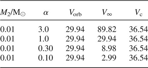
A list of the binary-single star encounters studied. α = V/V_orb and V_c is the critical velocity given by equation (3). M₂ is the planet mass. All velocities are given in km s₋₁.

Open in new tabDownload slide

Table 2.

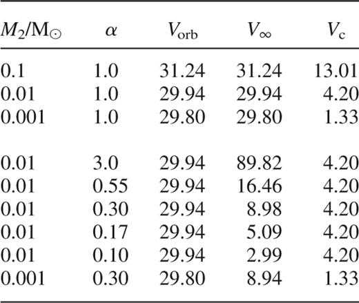
A list of the binary-binary encounters studied. α = V/V_orb and V_c is the critical velocity given by equation (4). M₂ is the planet mass. All velocities are given in km s⁻¹

Open in new tabDownload slide

(4)

where , is the binaries reduced mass, and d₁, d₂ are the semi-major axis of the binaries containing masses M_1,2, M_3,4, respectively.

Note for all simulations, , and . The turn-off mass for 47 Tuc is slightly lower than 1 M_⊙, probably , and the true encounter rates scale to be correspondingly slightly lower.

For each value of α, we simulated encounters for a range of impact parameters, ensuring that we considered sufficient large impact parameters to include all relevant interactions. For each set of encounters we then computed the cross-sections for the planetary system to be disrupted (i.e. the planet does not remain in orbit around either star), and for the orbit of the planet to be perturbed to eccentricities, , 0.1 and 0.3.

The cross-section for the breakup of the planetary system via encounters with a single star is shown in Fig. 1 as a function of α. Also shown is the cross-section for the two stars to pass within a distance, which was calculated using equation (1). Also shown is the breakup cross-section for rescaled assuming that the change in cross-section is purely an effect of the differing degree of gravitational focusing occurring for different values of α.

Figure 1.

The cross-section for breakup of the planet–star system as a function of (full curve), and for the intruding star to pass within the orbital separation of the planet–star system (dotted line). Both cross-sections are given in units of the binary separation (i.e. the cross-section of a target having a radius equal to the binary separation is π). The broken line is the breakup cross-section for rescaled assuming that the change in cross-section is purely an effect of the differing degree of gravitational focusing occurring for different values of α.

Open in new tabDownload slide

The cross-section for the breakup of the planetary system via encounters with binary stars shows a similar form to that seen in Fig. 1, except the value is increased by a factor of ∼2.

We consider now the cross-sections for the production of eccentric planetary systems. These are shown in Fig. 2 for encounters with single stars. The cross-sections are larger than the equivalent breakup cross-section. The cross-section for producing a planetary system with eccentricity being ∼ (see also Heggie & Rasio 1996). An important point to note here is that the systems with non-zero eccentricities can have semimajor axes larger than the initial circular orbit of the planet, and in any case the maximum separation (i.e. is certainly larger. A planet left in such an eccentric orbit is therefore a larger target for a subsequent breakup. We estimate that this will double the effective breakup cross-section for planets with initial separations . Systems left in extremely eccentric orbits tend to have equivalently large semimajor axes, this being the limit of systems that just failed to be broken up. The number of eccentric systems where circularization occurs will be small and limited to systems where the initial separation .

Figure 2.

The cross-section for the planet to be left in an eccentric orbit as a function of . Cross-sections are for systems with eccentricity , 0.1 and 0.3 (top to bottom). All cross-sections are given in units of the binary separation as in Fig. 1. The broken curve is the breakup cross-section for rescaled assuming that the change in cross-section is purely an effect of the differing degree of gravitational focusing ocurring for different values of α.

Open in new tabDownload slide

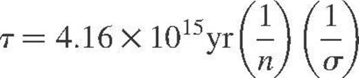
If we consider that V_∞ is a constant value for all sets of encounters, then the various values of α correspond to different values of orbital separation d. As and , . Considering , inspection of Table 1 reveals that corresponds to . Rescaling the other cross-sections for the same value of V_∞ we produce Figs 3 and 4, where now the cross-sections are given in units of (au)². These may be converted to time-scales via

Figure 3.

The cross-section for breakup of the planet–star system from encounters with single stars as a function of separation in au (full line), and for the planet to be left in an eccentric orbit with eccentricity, , 0.1, 0.3 (broken lines, from top to bottom).

Open in new tabDownload slide

Figure 4.

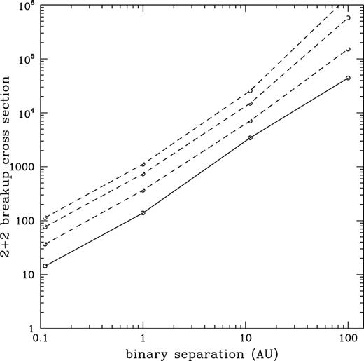
The cross-section for breakup of the planet–star system from encounters with binary stars as a function of separation in au (full line), and for the planet to be left in an eccentric orbit with eccentricity, , 0.1, 0.3 (broken lines, from top to bottom).

Open in new tabDownload slide

(5)

where n is the number density of stars (or binaries) pc⁻³, and σ is the cross-sections in units of (au)². In Table 3 we give the time-scales in years for systems to be broken up or left in eccentric orbits for both binary–single and binary–binary encounters, assuming a number density, , and 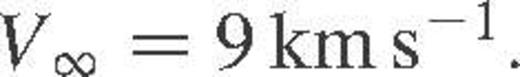. We will consider the implications for the survival, or otherwise, of planetary systems in stellar clusters in the discussion section.

Table 3.

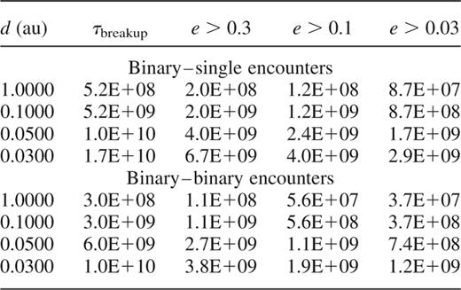
Time-scales (in years) for systems to be broken up or left in eccentric orbits for both binary-single and binary-binary encounters, assuming a number density, n = 10⁵ stars pc⁻³, and V= 9 kms⁻¹.

Open in new tabDownload slide

4.1 The importance of collisions

Thus far we have only considered exchanges and breakups as mechanisms to destroy planetary systems. For the very tightest systems collisions between the planet and a star or between two stars will also play a role. If two stars collide and merge, the planet will likely be swallowed up by the expanding merged object, assuming it remains bound to the collision product in the first place.

We computed the cross-sections for physical collisions or very close encounters between objects during an interaction. For encounters involving a single star, we find that mergers are unimportant except for encounters involving very tight planetary systems (i.e. where . For encounters involving binary stars, we find that the cross-section for mergers can be larger than the breakup cross-section for . For such tight planetary systems, we find that in units of (au)².

5 Discussion

Combining the cross-sections for breakups, significantly increasing system size (by making it eccentric), and collisions, we estimate that the effective cross-section for the destruction of tight planetary systems for encounters involving single stars, and for encounters involving binary stars. Assuming the core binary fraction in 47 Tuc to be , we therefore conclude that the effective destruction cross-section in the core is , for a planet in 0.4 au orbit. The data from the Hubble Space Telescope project will give the fraction of high mass-ratio main-sequence binaries in the same part of the cluster surveyed for planets.

Using equation (5), we are able to compute the likely time-scale for the destruction of a planetary system, or the time required to place the planet on an eccentric orbit. Assuming that a particular star–planet system is located within the core of 47 Tuc, where , we see that . We therefore require which is easily satisfied for most semimajor axes. A planet with an orbital separation would be broken up in ∼10⁸ yr. By comparison, a planet orbiting a star at the cluster half-mass radius will be somewhat less vulnerable. Here the number density hence we require only those systems where are likely to be destroyed. The critical value of d will clearly depend on the exact value of the number density of stars, n. Note that Sigurdsson (1992) assumed a stellar density ∼3 times smaller for 47 Tuc and derived a correspondingly longer time-scale for breakup in the core. Additional uncertainty is introduced by the time evolution of the 47 Tuc stellar density profile. If the cluster is evolving through normal relaxation, then it was substantially less dense in the centre a few billion years ago. However, there is some suggestion that the cluster may already have evolved through a dense core phase (Sills et al. 2000) in which case the rate of destruction of tightly bound planetary systems may have been an order of magnitude higher in the recent past. In either case, theory predicts little or no evolution in the stellar density near the half-mass radius, and the WF/PC2 field extends out from the core out almost to the half-mass radius. On the other hand, there are more stars to be observed in the denser parts of the cluster and the prior expectation therefore that most planets should have been found in the densest part of the observed field, assuming no dynamical disruption took place.

It should also be noted that simulations of the evolution of multiple planetary systems suggest that a relatively slight perturbation in the eccentricity of one or more planets may lead to a radical rearrangement of the system over a short time-scale (Quinlan 1992; Murray & Holman 1999). Thus we note that encounters that perturb the planets may play a role in the evolution of planetary systems, even in relatively low-density short-lived stellar clusters. For example, if , , for .

In terms of the current survey in 47 Tuc, it would seem possible that all planetary systems have been destroyed if all the stars in the survey were located in the highest-density regions. Given that some of the stars observed are in regions with an order of magnitude smaller stellar density, it is difficult to explain away all the expected detections. However, there are fewer stars observed in the low-density regions of the cluster, so if the intrinsic specific density of 51 Peg-like systems is somewhat lower than in the solar neighbourhood, then we might have expected more like 5–10 detections from observing 34 000 stars, and 75 per cent of those in the densest regions. In order for direct dynamical disruption to explain the absence of 51 Peg-like systems, one still requires either a past denser phase for the core, or a very long time spent at the current density. The minimum average density for the environment of a given planetary system required for its destruction being . From our calculations here, we conclude that tight planetary systems (i.e. d ≲ 0:1 au) will definitely survive in less-dense clusters where subsequent surveys should be conducted. An ideal target is NGC 6352. It has core density of about 10³ stars pc⁻³, is at an estimated distance of 6.1 kpc (compared with 4.6 kpc for 47 Tuc) and has metallicity (compared with −0.71 for 47 Tuc). With the Advanced Camera on the Hubble Space Telescope, a considerably wider field can be monitored, and another survey for transits carried out.

Acknowledgments

MBD gratefully acknowledges the support of a URF from the Royal Society. SS gratefully acknowledges support from NASA through grants STSCI GO-7307 and GO-8267.

References