


Abstract
We present a comparison between a plasma-generated ‘starting jet’ experiment and an axisymmetric numerical simulation of the flow. The experimental flow and the numerical simulation give results that agree both qualitatively and quantitatively, showing that the complex vortical structures arising in the flow are surprisingly well reproduced by the numerical model. This result inspires confidence in the accuracy of astrophysical jet numerical simulations. Also, even though the Mach number of our laboratory jet is somewhat low (M∼0.5), the dimensionless parameters of this jet are not very far from those expected for Faranoff–Riley class I radio jets.
1 Introduction
The Faranoff–Riley class I radio jets are thought to correspond to relatively low Mach number (M∼0.5–), collimated flows (see for example Bicknell 1985). These flows have been modelled analytically as fully turbulent flows, using a ‘turbulent viscosity’ approach for a description of the turbulence (Bicknell 1984, 1986a,b; Komissarov 1988, 1990a,b). A more sophisticated ‘k–ε’, second-order closure model for the Reynolds stresses (Dash, Wolf & Seiner 1985) has been used in axisymmetric numerical simulations of radio jets by Falle (1994).
Though such parametrizations can be properly calibrated with laboratory jet experiments (Dash et al. 1985; Cantó 1991), they are somewhat questionable when applied to astrophysical jets. Interestingly, the problem with these parametrizations does not arise from the intrinsic differences between radio jets and the laboratory jets used to calibrate the parametrizations, but are a direct result of the nature of astronomical observations.
The two dimensionless parameters that fundamentally determine the properties of a non-radiative jet are its Mach number M and its Reynolds number Re. Laboratory experiments range from M≪1 to M∼20, covering a large part of the Mach number range expected for astrophysical jets. Also, laboratory jets easily have Reynolds numbers of Re>105 placing them in the ‘high-Re regime’, in which the nature of the flow stops depending on the actual value of Re. It is generally assumed that astrophysical jets also are in this high-Re regime. Therefore, a calibration of a turbulence parametrization based on laboratory experiments should indeed be applicable for (at least non-radiative) astrophysical jets.
However, the problem is that in general the aim of turbulence parametrizations is to allow a calculation of the correct ‘mean flow’, averaged over times long enough so that the time-dependent turbulent eddys are smoothed out. Such a mean flow is of course relevant for obtaining the drag, lift, etc. for aerodynamic objects, and can be obtained through long enough time-averages of the flow variables in a laboratory experiment. Astronomical observations will clearly always be inappropriate for computing such a mean flow, as the difference between the time-scales relevant for radio jets and for humans is of ∼4 orders of magnitude (this number coming down to only a factor of ∼10 for the much faster evolving Herbig–Haro jets).
Therefore, observations of astrophysical jets will always correspond to ‘snapshots’ in which the detailed structure of the turbulent motions is evident, and may well be more conspicuous than the structure of the underlying mean flow. Because of this, models of jets based on parametrizations of the turbulence are difficult to compare with astronomical observations.
The alternative option is to carry out direct simulations of the jet flow, in which at least the larger turbulent eddys are appropriately resolved, and hopefully correctly followed by the numerical intergration. Such a simulation could include a parametrization of the effects of the subgrid resolution turbulent eddys, following the large eddy simulation (LES) approach which has been well studied in the atmospheric sciences (Smagorinski 1963; Deardoff 1970; Lilly 1987). To parametrize the subgrid turbulence, the eddy viscosity ν is expressed as a function of the grid size and the velocity shear, in contrast to a ‘standard’ mixing length model (see, for example, Cantó & Raga 1991), in which the eddy viscosity is assumed to be proportional to the characteristic size of the turbulent region (rather than to the grid size of the simulation). Alternatively, there are ‘second order closure’ models for the subgrid turbulence, which qualitatively resemble the k-ε model described above, but are calibrated to only account for the subgrid turbulent flow (following the philosophy of the LES approach). As calibrations of LES parametrizations appropriate for astrophysical jet flows have not yet been carried out, the implementation of LES models for these flows will involve a detailed experimental and theoretical study.
One of the most critical points of the LES parametrization is the predictability problem, i. e., the propagation to large scales of the uncertainty contained initially in the subgrid scales. The subgrid fluctuations, parametrized in the initial condition, can affect the evolution of the flow at large scales. Normally, and fortunately, this occurs after a delay time known as the ‘predicability time’ (Lesieur 1995). In other words, a LES turbulence simulation, however good the subgrid scale modelling, will only describe the large-scale flow evolution for a time smaller than the predictability time. This means that there is no turbulence parametrization which is ‘a priori’ better than the others, the main criterion for choosing between different parametrizations being a comparison of well calibrated models with experimental results. As we currently do not have appropriate experimental data for carrying out such comparisons, in the present paper we discuss ‘direct’ numerical simulations (i. e., with no parametrization of the subgrid turbulence). Such simulations have been computed many times for modelling radio jets (see, for example, the old simulations of Norman et al. 1982, and the review of Ferrari 1998), and it has been shown that jets with M<3 develop very complex structures, with shock waves within the jet beam and vortex shedding at the head of the jet.
The results from the available simulations are of course somewhat questionable on a number of grounds (see, for example, Falle 1994; Raga 1994). The two main drawbacks of the simulations areas follows.
- (i)
Most of the simulations are 2D (axisymmetric), and it is not clear to what extent the resulting structures correspond to the real, 3D turbulent flow. Recent studies (Bodo et al. 1998), showed that important differences between 2D and 3D simulations are found. The most evident are (1) the more rapid and effective mixing in the 3D case (as a result of the faster growth of the small-scale structures) and (2) the larger broadening of jet in the 3D case. The latter effect is particularly evident at high Mach numbers (M=10 in the paper of Bodo et al. 1998).
- (ii)
As a result of the limited computational resolution of the simulations, their effective Reynolds numbers typically have Re<100 values, very far from the high-Re regime (Re>105)
While the second of these problems is still present in the more recently published axisymmetric jet simulations (see, for example, Komissarov & Falle 1998), 3D simulations of turbulent jets are now beginning to be studied (e.g. Bodo et al. 1998), albeit at low Re.
In the present paper we describe a comparison between an axisymmetric jet simulation and a laser generated ‘starting jet’ experiment. Through this comparison, we can evaluate the qualitative and quantitative successes of the numerical simulation at reproducing the complex vortical structures that develop in the jet. The experiment is described in Section 2. The numerical simulation is described and compared with the experimental results in Section 3. Finally, a comparison between the parameters of the laser-generated jet and the ones of type II radio jets is given in Section 4.
2 The Laser-Generated ‘Plasma in a Bottle’ Starting Jet Experiment
We have carried out a ‘starting jet’ experiment, in which we follow the initial phases of the time-evolution of the jet flow. With a laser pulse, we generate a high temperature, partially ionized plasma bubble within an ≈1 cm diameter glass bottle. This bottle has a ≈3 mm diameter exit nozzle. First to emerge through this nozzle are the shock waves pushed out by the plasma bubble, at later times the hot gas (which was initially heated by the laser pulse) exits in the form of a very well collimated jet.
A schematic diagram of the experimental setup is shown in Fig. 1. Electric breakdown in air was obtained by focusing (with a 7.5-cm focal length plano-convex lens with anti-reflection coating) a beam from a Q-switched Nd:YAG laser source (Continuum, model Surelite II),1 operated at λ=1.06μ with a 10-Hz repetition rate, a 7-ns pulse width (full width half-maximum – FWHM) and a 6-mm beam diameter. The energy was varied in the 50–150mJ range (though the particular experimental results discussed below correspond to a 100-mJ pulse energy) and was measured with an energy metre (LabMaster Ultima with crystalline pyroelectric sensor LM-P10i from Coherent)2 EM1 through a calibrated beam splitter BS1 (see Fig. 1). The transmitted energy was measured with an additional power and energy metre (Scientech, model 365)3 EM2 (see Fig. 1).
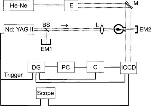
The setup of the laser-generated starting jet experiment. A focused Nd:YAG laser pulse produces a high pressure plasma bubble within a glass bottle. Shadowgrams of the flow that emerges through the nozzle of the glass bottle are obtained by imaging an expanded He-Ne laser beam with an ICCD. The notation used in the diagram is as follows: E (expansor), M (mirror), BS (beam splitter), DG (delay generator), C (controller), ICCD (intensified CCD), L (lens), EM (energy metre), OD (optical detector).
The region directly outside the exit nozzle was illuminated with an expanded beam from a He–Ne laser emitting at λ=632.8 nm (JDS Uniphase, model 1125P)4 with a power of 10 mW. After going through the region with the flow, the probe beam was imaged with a 1024×256 intensified charge-coupled device (ICCD) camera (PI-MAX:1024UV from Princeton Instruments)5 with a gate width of less than 5 ns, and the signal was stored in a computer. This camera was synchronized with the pulsed laser using a Stanford delay generator model DG-5356 and the delay was measured through a photodiode connected to a 500-MHz digital oscilloscope, Tektronix model TDS 524 A7.
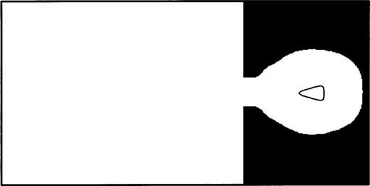
With this experimental setup, we were able to obtain shadowgrams at a series of different time-delays with respect to the Nd:YAG laser pulse. Actually, in order to improve the signal-to-noise ratio of our shadowgrams, we have taken the mean of ten 1-μs ICCD exposures for each of the different time-lags that we have obtained measurements for (though the observed flow structures are also seen in the individual exposures). The resulting shadowgrams reveal the structure of the flow that exits through the nozzle of the glass bottle (see above and Fig. 1). However, we were unable to obtain shadowgrams of the flow within the glass bottle, because of the uneven refraction of the laser beam in going through the low optical quality glass walls.
3 The Numerical Simulation
In this section, we present a comparison between the experiment described in the previous section and a numerical simulation of the flow. This numerical simulation has been done with the axisymmetric version of the yguazu´-a adaptive grid code (which is described in detail by Raga, Navarro-González & Villagrán-Muniz 2000). This code integrates the gas–dynamic equations (together with a set of rate equations for microphysical processes) with a second-order accurate (in both space and time) version of the ‘flux vector splitting’ algorithm of Van Leer (1982). A binary, hierarchical adaptive grid is used, which automatically refines and de-refines depending on the magnitude of the round-off error (estimated by comparing the results obtained in two successive grid resolutions; see Raga et al. 2000).
In order to compute a numerical model for the laser-generated jet, we have digitized the shape of the glass bottle, and imposed a reflection condition on this surface. We start the numerical simulation by filling the computational domain with a uniform, stationary atmosphere with a density ρ0=10−3 g cm−3 (which is the atmospheric density at a height of 2100 m above sea level of Mexico City), and temperature T0=300K, except for a conical region centred within the glass bottle, which is set at a temperature T1=25 000K (and at the same density ρ0). This conical region has a half-opening angle α=15°, and a length l=2.8 mn, with the base of the cone placed at a distance h=4.2 mn, from the bottom of the glass bottle. This initial configuration is shown in Fig. 2.
A schematic diagram showing the initial configuration for the numerical simulation. The region shown has a size of 4×2 cm (measured horizontally×vertically), corresponding to a 4×1 cm(axial×radial), cylindrically symmetric computational domain. The whole of the domain is initialized with a ρ0=10−3 g cm−3 density, and temperatures T1=25 000K (within the cone inside the glass bottle) and T0=300K (for the rest of the domain). The digitized shape of the glass bottle is shaded in black, and a reflection boundary condition is imposed on the edge of the shaded region. A free outflow condition is imposed on the remaining boundaries of the computational domain.
In previous papers (Raga et al. 2000; Sobral et al. 2000), we have shown that numerical simulations initialized with this ‘hot cone’ initial configuration reproduce the flow resulting from a laser-generated plasma bubble in the free atmosphere very well. It is therefore well-justified to use the same initial condition for modelling the more complex ‘plasma in a bottle’ experiment described in Section 2.
Starting from these initial conditions, we integrated the gas–dynamic equations with the yguazu´-a code (see above and Raga et al. 2000). For this calculation, we have used a five-level, binary adaptive grid with a maximum resolution of 0.078 mm (in both the axial and radial directions), in a 4×1(axial×radial) computational domain. A constant specific heat ratio, γ=1.4, has been assumed.
The time-dependent density stratification resulting from the numerical integration is shown in Fig. 3. In the t=2-μs frame, we see the shock wave driven out by the overpressured plasma cone not yet reaching the walls of the glass bottle. At t=100μs, part of this shock wave has exited through the nozzle, and left the computational domain. Other compression waves are seen to be still travelling through the domain. These compression waves are the result of a series of reflections of the initial blast wave on the inner walls of the glass bottle. For t⩾100μs, the air heated by the laser pulse starts to exit through the nozzle, forming a very well collimated jet that travels through the computational domain. This jet develops a series of ring vortices.
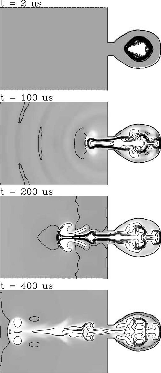
Time-evolution of the density stratification resulting from the numerical simulation. The density stratifications for times t=2, 100, 200 and 400 μs from the laser pulse are shown. The density stratification is shown with linearly spaced contours (at intervals of 10−4 g cm−3) and with a grey-scale (with darker tones corresponding to higher densities). The stratifications correspond to a cut of the cylindrical density structure through the symmetry axis, and the vertical dimension of the plots is 2 cm.
A comparison between the ‘numerical’ and the corresponding ‘experimental’ time-evolutions is shown in Fig. 4. This comparison can only be made for the flow that is exiting the bottle through the nozzle, since our experimental setup does not allow us to observe the flow within the glass bottle (see Section 2). From Fig. 4, one sees that there are many similarities between the two time-series:
- (i)
between t=0 and t=80μs, four distinct compression waves leave the exit nozzle and travel through the observed domain,
- (ii)
at t≈50μs, the air bubble initially heated by the laser starts to leave the glass bottle,
- (iii)
at t≈80–90μs, the leading edge of the hot air jet starts to develop a well defined vortex ring,
- (iv)
at t≈180μs, this vortex ring develops a swept-back ‘tail’, which curves away from the jet beam.

Comparison between the numerical simulation and the ‘plasma in a bottle’ starting jet experiment. The two left columns correspond to cuts through the symmetry axis of the density stratification obtained from the numerical simulations (with darker shades of grey corresponding to the denser regions) for different times from the laser pulse (each graph being labelled with the time in μs). The two right columns show the shadowgrams obtained from the experiment for the same times as the corresponding graphs from the first two columns. The domain shown in each of the ‘theoretical’ graphs (first two columns) has a size of 1.6×1.6 cm with the exit nozzle of the glass bottle (see Figs 2 and 3) being immediately to the right of the domain. The ‘experimental’ graphs (second two columns) show a circular domain of 1.6-cm diameter, also with the exit nozzle immediately to the right of the domain (note that small displacements of this circular domain on the CCD detector have occurred during the experiment).
We should note that the experimental results shown in Fig. 4 have the following problem. During the experiment, small displacements of the charge-coupled device (CCD) camera occurred, so that the circular aperture (to the right of which is the exit nozzle of the glass bottle) does not always fall in the same place on the surface of the CCD detector. Because of this, in order to evaluate the position of the head of the jet as it travels away from the exit nozzle, it is necessary to measure the distance from the jet head to the left edge of the circular aperture (which is always visible in the shadowgraphs, see Fig. 4). One can then compute the distance from the exit nozzle using the known 1.6-cm diameter of the circular aperture.
Of course, in a more quantitative analysis some differences between the numerical and experimental results are evident. As an example, in Fig. 5 we show the distance from the exit nozzle to the leading edge of the jet (computed as described above), and the width of the leading vortex ring as a function of time. From this figure, we see that while the propagation of the leading edge of the hot gas jet is well reproduced by the numerical simulation (except for a ≈0.5-mm offset which could be an error in the zero-point of the positions measured in the experiment), the width of the vortex ring in the experiment appears to reach widths greater by ≈1 mm than the ones reached by the vortex ring in the numerical simulation.
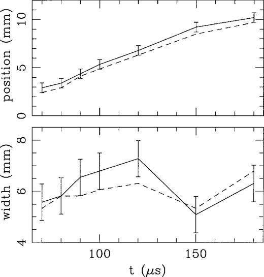
Distance from the exit nozzle to the leading edge of the hot air jet (top) and full width of the leading vortex (bottom) as a function of time from the laser pulse. The width of the vortex has been measured at a position of 1.2 mm upstream from the leading edge of the jet. The experimental results (with error bars) are shown with the dashed lines, and the corresponding results obtained from the numerical simulation are shown with the solid lines.
4 Conclusions
We have presented a comparison between a laser-generated plasma jet experiment and an axisymmetric simulation of the flow. We show that the experimental and numerical structures of the jet flow agree surprisingly well in a qualitative way. A main vortex is generated at the head of the jet, and the time-evolving morphology of this vortex is well reproduced by the numerical simulation. Even some more quantitative comparisons between the properties of the jet and the results of the simulations are moderately successful (see Fig. 5).
From this comparison between a numerical model and a laboratory jet, we conclude that a ‘direct simulation’ (in which no effort is made to parametrize the effects of the turbulence) quite successfully reproduces the larger vortical structures formed in the jet flow. Because of this, we are surprised to find ourselves disagreeing with Falle (1994), and have to conclude that at least the initiation of the vortex-shedding in the head of a jet appears to be well reproduced by a ‘standard’, axisymmetric jet numerical simulation.
Of course, while our simulation and experiment are at most transonic (see below), the simulations of Falle (1994) are hypersonic. It would therefore be interesting to perform experiments in which the Mach number can be modified in a controlled way, in order to see the possible changes in the development of the turbulence with Mach number. We plan to carry out such experiments in the future by enclosing the glass bottle and surrounding space in a vacuum chamber, and lowering the temperature of the air by substantially reducing the pressure in the chamber.
Moreover, we note that the eddies having the largest sizes in a turbulent flow contain the larger part of the kinetic turbulent energy. The size of the largest eddy, in a first approximation, provides quantitative estimations of the intensity of the turbulence in a fluid. Although our present model has no turbulence parametrization, the small average relative error (of ≈8 per cent, see Fig. 5) found in the measured size of the largest eddy in our simulations indicates that a ‘direct simulation’ produces reasonable results, at least for the parameters of our starting jet experiment.
In order to better estimate how well the model reproduces the turbulence, one could imagine future experiments in which all the turbulence energy scales are measured. A possibility would be to measure, in a statistical way, the random fluctuations of a laser beam propagating through the turbulent flow. The wavefront perturbations are strictly correlated to the turbulence intensity in the flow (Tatarski 1961), so that estimations of the properties of the turbulence could be obtained from such an experiment. Such estimations could then be used to calibrate a turbulence parametrization.
In order to quantify to what extent our plasma-generated jet is directly comparable to astrophysical jets, we note the following:
- (i)
when the hot air starts emerging from the nozzle (at t≈70μs, see Fig. 4), the out-flowing material has Mach numbers of M≈0.5, dropping to M~;0.1, at t=200μs,
- (ii)
the jet material is in approximate pressure equilibrium with the surrounding atmosphere, and its density is ∼30 per cent lower than the one of the surrounding environment,
- (iii)
the Reynolds number of the out-flowing gas (computed with M = 0.5 and the diameter of the nozzle) has a value Re≈2×10⁴ which is high but does not place the flow in the high-Re regime.
The properties of the jet flow are also illustrated in Fig. 6, where we show cuts across the diameter of the outflow nozzle of the Mach number, density, pressure and temperature for a time t=70 μs. From this Figure, we see that at this time the jet has an almost top-hat Mach number cross-section, and that the central region of the jet has a lower density and higher temperature than the edges of the beam (while keeping the pressure constant to within ≈7 per cent, see Fig. 6).
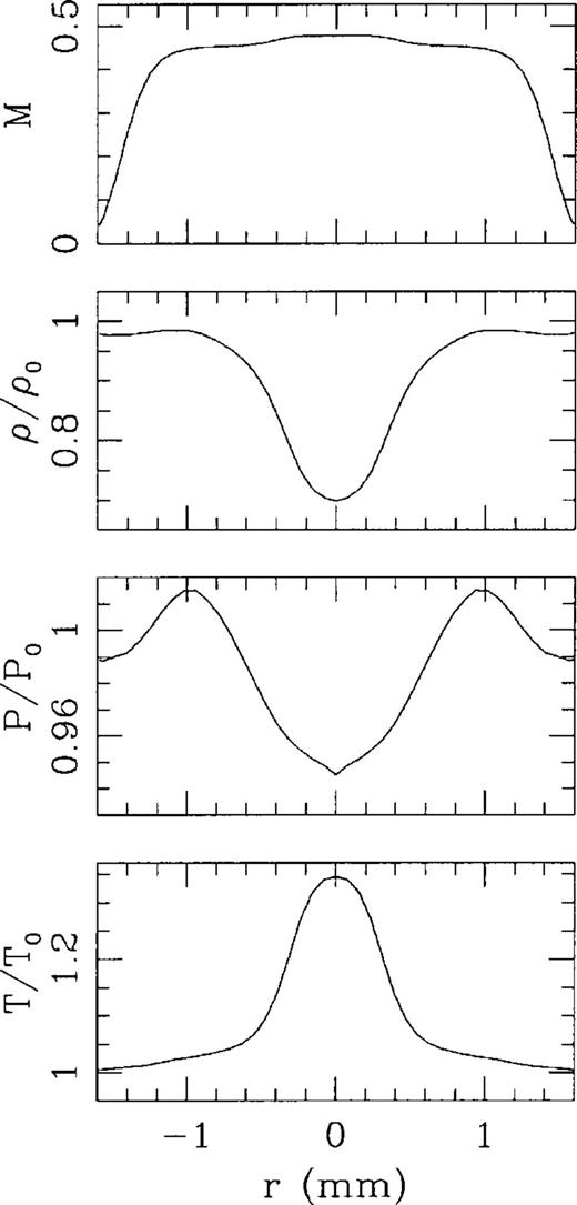
Top to bottom: Mach number, density, pressure and temperature cross-sections across the outer edge of the exit nozzle of the glass bottle (see Fig. 2). The cross-sections shown have been extracted from the t=70μs time-frame of the numerical simulation. The density, pressure and temperature have been normalized to the values of these variables in the free atmosphere.
Therefore, the astrophysical jets with parameters closest to our laboratory jets are the Faranoff–Riley class I radio jets, which are normally modelled as relatively low Mach number flows. However, radio jets are generally thought to be much less dense than the surrounding environment, which is clearly not the case in our laboratory jet (see Fig. 6 and the above discussion).
Acknowledgments
This work was supported by the DGAPA (UNAM) grants IN 102796, IN 110998, IN 118199, IN 119999 and IN 128098, and the CONACyT grants 32753-E, 27546-E, 32531-T and J32412-E. AR acknowledges support from a Fellowship of the John Simon Guggenheim Memorial Foundation. We thank Salvador Ham-Lizardi for the design and manufacture of the glass bottles for the plasma-generated jet experiments. We also thank an anonymous referee for helpful comments about the paper.
References
1Continuum, Santa Clara, California, USA.
2Coherent, Santa Clara, California, USA.
3Scientech, Boulder, Colorado, USA.
4Uniphase, San Jose, California, USA.
5Kodak, Rochester, New York, USA.
6Sunnyvale, California, USA.
7Tektronix, Beaverton, Oregon, USA.
