A speedy pixon image reconstruction algorithm Free

Abstract

1 Introduction

The process of measuring an image can, for many applications in astronomy, be written as

(1.1)

where x represents a pixel position in a two-dimensional array, or image, D is the observed data, T is the true image, B is the point spread function (psf) of the measuring instrument, assumed to be invariant across the image, with N being the associated statistical noise and * represents the convolution operator such that

(1.2)

where n is defined to be the number of pixels in the data image. The task of an image reconstruction algorithm is to infer the true image given the data, knowledge of the psf and the statistical properties of the noise. For the simple case when there is no noise then, assuming that the inverse of the beam exists, that there is no structure on subpixel scales and ignoring complications introduced by edge effects, the inferred truth, T̂, can be obtained using the convolution theorem and will exactly equal T. Denoting the Fourier transform of f(x) by f˜(k), T̂ can be found by inverse transforming

(1.3)

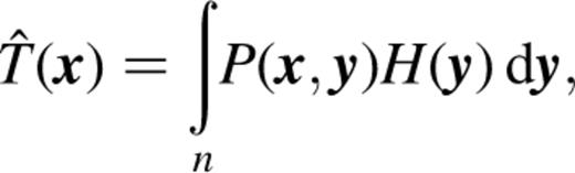
The n pieces of information in the data allow a perfect reconstruction of the n pixel values in the truth. With noise switched on, the number of degrees of freedom in the solution increases by n, while the number of constraints remains fixed, yielding an ill-posed problem. Thus, the job of the reconstruction algorithm becomes to decide which of the possible inferred truths is the best, whatever that may mean.

An extension of the simple case described above involves filtering the data to remove the noise before inverse transforming equation (1.3) to yield T̂. One particular, widely used example of this is the Wiener filter (Wiener 1949; Rybicki & Press 1992; Bunn et al. 1994; Lahav et al. 1994; Fisher et al. 1995). This procedure is non-iterative (it iterates to and the final inferred truth is completely determined once guesses for the power spectra of the true signal and the noise components have been made. If the assumed power spectra are correct then the resulting filter will minimize over the whole image the variance between the reconstructed and true signals. It can also be shown that the Wiener filter yields the maximally probable inferred truth if the true and noise values are normally distributed (Rybicki & Press 1992). For situations where these distributions are not Gaussian, the optimal filter differs from the Wiener filter. While the Wiener filter method involves only a few transforms, and is thus rapid, it would in general be desirable to break the degeneracy in solution space with a technique that both does not require any assumption about the nature of T and produces optimal images for any true signal distribution.

Another type of transform is the wavelet transform (e.g. Slezak, Bijaoui & Mars 1990) where the inferred truth is described using a set of basis functions designed to extract information on a variety of scales. Once again, this is a linear method that involves applying a transformation to the data in order to extract information about particular scales of interest.

An alternative approach to image reconstruction involves quantifying the acceptability of a particular inferred truth, then iterating the inferred truth until it becomes maximally acceptable. One reasonable demand to make of T̂ is that the resulting distribution of residuals, defined as

(1.4)

is statistically indistinguishable from that of the anticipated noise N, i.e. requiring a ‘good fit’ to the data. The particular statistic used to describe the extent of the misfit will depend on the nature of N. For example, χ² is a frequently employed statistic when noise values are drawn from a normal distribution.

Having chosen a misfit statistic, approaches to reducing further the acceptable solution space are more varied. A common and simple route is to parametrize T̂ and use the data to fit a small number of parameters. This is very quick and effective, provided that the prejudice contained in the parametrization is appropriate. For complicated images, a more sophisticated procedure is desirable.

To understand better where pixons fit into the story, consider the following conditional probability equation with M representing all aspects of the model used to transform T̂ to D:

(1.5)

This is merely the probability of having a particular combination of data, model and inferred truth, divided by the probability of obtaining a particular data set. Since D is measured before it is used to infer T̂, p(D) is constant. In addition, the desire to avoid introducing prejudice requires that p(M) is constant over all models. This leaves

(1.6)

On the left-hand side of this proportionality is the quantity that one would like to maximize in the reconstruction, namely the probability of a combination of inferred truth and model given the data. The first term on the right-hand side is readily identified as the ‘likelihood’, and the second term is commonly called the ‘image prior’. From a Bayesian viewpoint, it is reasonable to associate a probability to the plausibility of obtaining a particular inferred truth once a model is specified, despite the non-repeatable nature of the image prior. This provides additional leverage in the quest to reduce the acceptable solution space. Note that even if the model is held fixed and one seeks to maximize p(T̂|M,D) the above equation looks very similar because in that case and

In order to quantify the image prior, consider the situation of distributing Z indistinguishable photons randomly among q buckets. Denoting the number of photons in bucket i by z_i, the probability of a particular distribution is

(1.7)

The most probable choice of {z_i} can readily be shown to be the one that has the same number of photons in each bucket. This probability also increases when the number of buckets is decreased; an Occam's razoresque tendency to favour simple descriptions. Referring back to the image prior, p(T̂|M) will be increased by having the photons distributed evenly through the model buckets, and by reducing the number of buckets.

This approach to image reconstruction was pioneered by Skilling (1989) and Gull (1989). By analogy with statistical thermodynamics, they related the maximization of the image prior to a maximization of the entropy of the reconstructed truth. In the absence of additional information which could shift the prior away from the default flatness, uniform T̂s are preferred over more complicated images that require a less probable distribution of the indistinguishable photons in the image pixels.

These maximum-entropy methods (MEM) are conventionally applied in the pixel grid in which the data are measured. However, if the real truth deviates from flatness then, to the extent that the image prior is important relative to the likelihood term in equation (1.6), this procedure will bias T̂ away from T. This suggests that the distribution of buckets into which the photons are placed should be set according to the measured distribution D if the prior probability is to be truly maximized. Furthermore, one implication from the above discussion is that the number of buckets should be minimized in order to create the simplest, and consequently most plausible, description for T̂, rather than using n parameters because this is how many pixels there are in the data image. Considerations such as these led Piña & Puetter (1993; hereafter PP93) to introduce the pixon concept. Unlike the uniformly arranged pixels, pixons are able to adapt to the measured D in order that the information content is flat across the inferred truth when described in the pixon basis. This adaptive ‘grid’ essentially uses a higher density of pixons to describe the inferred truth in regions where more signal exists, and only a few very large independent pixons for the background, or low signal-to-noise ratio (SNR) parts of an image. Relative to MEM, the pixon method allows the probability in equation (1.6) to maximize itself with respect to one aspect of the model which conventional MEM keep fixed. The task of maximizing p(T̂,M|D) boils down to finding the inferred truth containing the fewest pixons, which nevertheless provides an acceptable fit to the data. Operationally, the main difference between MEM and the pixon method is that MEM explicitly quantifies the image prior and does a single maximization of p(T̂|M,D). In the pixon case this is split into successive likelihood and image prior maximizations. Both MEM and the pixon method require an assumption to be made concerning the noise distribution in order that the goodness-of-fit can be quantified.

In summary, the pixon method is an iterative image reconstruction technique that produces inferred truths that are smooth on a locally defined pixon scale, and the iterations have a well-determined finishing point, namely when the pixon distribution has converged to the simplest state that yields an acceptable fit to the data. This approach to image reconstruction has been applied to a variety of astronomical data sets (e.g. Smith et al. 1995; Metcalf et al. 1996; Dixon et al. 1996, 1997; Knödlseder et al. 1996). A detailed discussion of the theoretical basis of the pixon, and a list of applications of the method, can be found in the paper by Puetter (1996).

In the original pixon implementation described by PP93, the time taken to perform a reconstruction was such that, for images containing at least 256² pixels, reconstructions would be impractically slow. While the discussion so far shows in principle the advantages offered by the pixon approach, the implementation of the idea remains to be specified. The main purpose of this paper is to describe a speedy pixon algorithm that is capable of reconstructing 256² pixel images in a few minutes on a workstation. In Section 3 the method is applied to two simulated astronomical data sets. The results are compared with a simple maximum-likelihood (ML) method and the robustness of the reconstructions is tested quantitatively using Monte Carlo simulations. Puetter & Yahil (1999) have reported the existence of accelerated and quick pixon methods. These are also considerably faster than the original pixon algorithm of PP93.

2 Method

2.1 Outline

The speedy pixon algorithm does not differ greatly from that originally proposed by PP93. Namely, the maximization of the probability in equation (1.6) is performed in an iterative fashion with each step consisting of a change in the number of pixons being used to describe the inferred truth followed by a conjugate gradient maximization of the likelihood (or equivalently minimization of the misfit statistic) for the fixed pixon distribution. These iterations are stopped when the inferred truth is described using the fewest pixons that allow an adequate fit to the data. The details of the pixon implementation are given in the following section, before considering how they impact upon the minimization of the misfit statistic. A flow diagram outlining the entire procedure is shown in Fig. 1.

Figure 1.

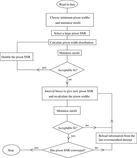
Flow diagram showing the structure of the algorithm. There is an initial ML type of fit, with all pixon widths taking the minimum available value. The resulting pseudo-image is used to find a pixon SNR that is too large to enable an acceptable fit to be found. Then the largest pixon SNR giving rise to an acceptable residual distribution is found by interval bisection.

Open in new tabDownload slide

2.2 Specifics of the pixon implementation

For the examples described in Section 3 the inferred truth is reconstructed in the same grid as the observed data and thus contains n values, one for each pixel. Given that the pixons are to be less numerous than the pixels, these n evaluations of the inferred truth cannot be independent. In practice a pseudo-image H is defined in the pixel grid and T̂ is evaluated by correlating the pseudo-image values over a region with a size determined by the local information content. This can be written as

(2.1)

where P(x,y) is a weight function, the pixon shape, defining how much signal the inferred truth at pixel x gathers from the pseudo-image at y. From this equation it can be seen that T̂(x) merely represents the result of convolving the pseudo-image with the pixon shape appropriate to pixel x. Thus, provided the number of distinct pixon shapes is finite and independent of n, it is already apparent why the time to compute the misfit statistic, or the derivatives with respect to the pseudo-image, is going to scale like n log n. If each pixel were allowed a separate pixon width then the time taken by these calculations would have an extra factor of n in the scaling, so it is very desirable to impose a limited set of available pixon widths.

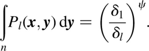
The choice of pixon shapes and sizes will place constraints on the types of truths that could possibly be recovered. Thus, using the vocabulary adopted by Puetter (1996), it is important that the richness in the pixon language is sufficient to enable a wide variety of truths to be reconstructed. After all, it should be the data that drives the reconstruction algorithm to an inferred truth, rather than the algorithm knowing beforehand what it is going to see! For the reconstructions presented in Section 3, a set of n_pixon circularly symmetric two-dimensional Gaussians was used with widths, truncated at This pixon shape was found to give better results than either an inverted paraboloid or a top hat for the examples considered. These alternative pixon shapes produced less smooth reconstructions, with the ‘edges’ of pixons being more apparent. While the smoother reconstructions produced with Gaussian pixons were preferable for the examples considered in this paper, the particular pixon shape being adopted should depend on the nature of the image being reconstructed.

Constructing T̂ in this way it was found that, for the examples described in Section 3.2 where there is one strong source which is sharply peaked, the pseudo-image was high in the pixel at the position of the source, and essentially zero in all surrounding pseudo-image pixels. Even with this extremely sharp pseudo-image, the inferred truth was still too smooth to fit the data. The surrounding pixels were gathering too much signal from the central spike in the pseudo-image, yet the central pixel needed to have more signal to match the underlying spiky source. Thus the pseudo-image had very little freedom and the reconstructed image was determined by the richness in the chosen set of pixon widths. To provide a little more flexibility to the pseudo-image in such a situation, the normalization of the lth pixon was chosen such that

(2.2)

With this means that in pixels having large pixon widths, the inferred truth will be suppressed relative to that calculated when all pixons are normalized to the same value. The pseudo-image values in the low signal regions, where the larger pixons are being used, are thus encouraged to increase relative to those in the high signal parts of the image. An unpleasant side effect of this is that the T̂ values in high signal pixels can become unduly influenced by the boosted regions of the pseudo-image, so in calculating the signal, the following weights were also included:

(2.3)

such that

(2.4)

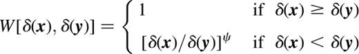
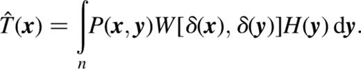
This down-weights the contribution to T̂ gathered from the pseudo-image pixels with larger δs. Values of ψ between 0 and 1 were used for the reconstructions in Section 3. The introduction of this extra weight means that the calculation of T̂ no longer involves just a single convolution. However, by splitting the integral into n_pixon separate convolutions of P_l with a Wδ_l,δ(y)]-weighted H, the n log n scaling of the misfit calculation can be preserved.

The procedure for defining the distribution of pixon widths is based on the desire to have the same amount of information in each pixon. Information content can be parametrized through a pixon SNR. This is defined as

(2.5)

σ(y) is the anticipated amplitude of the noise in pixel y. The final term just represents the removal of the non-normalization of the pixons, and the first δ(x) is there because the mean SNR within the pixon is being calculated. For a specified pixon SNR, the pixon width distribution is chosen such that all pixels have the minimum available δ that provides at least the required SNR. This differs from the fractal pixon basis approach (Puetter & Piña 1993), where the pixon SNR is not kept constant across the entire image.

For the reconstructions described in Section 3.2, it was found that relaxing the need for the inferred truth to have a constant SNR in each pixon led to superior results. With a flat inferred truth in the pixon basis, the higher signal regions of the data image received larger, and thus less likely, reduced residuals. In order to decrease this discrepancy, the required pixon SNR was decreased in the high signal pixels. The pixon SNR appropriate for pixel x was defined to be f_SNR(x) times the global value, where

(2.6)

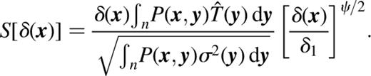
with r(x) being the convolution of with the correctly normalized pixon appropriate to each pixel, and υ a constant chosen to lie in the range [0,1]. While this is a very ad hoc addition to the method, it encapsulates the desire to provide more freedom in the badly fitting regions of the reconstructed image, rather than keeping rigorously to the maximum-entropy flat T̂ solution. This is similar in spirit to the fractal pixon basis introduced by Puetter & Piña (1993).

The remaining part of the pixon story, is to describe the fashion in which the pixon SNR is iterated. To define the first T̂, in order that the SNR can be computed via equation (2.5), a maximum-likelihood-type fit is performed using and starting from a flat T̂ with the mean value of D. An initial pixon SNR is chosen such that the resulting pixon distribution has too few degrees of freedom to allow a good fit to be obtained. Interval bisection is then used to find the maximum acceptable pixon SNR. At each stage, the last over-smoothed (i.e. badly fitting) T̂ is used to infer the new pixon distribution. This decreases the chance of introducing spurious structures into the reconstruction. In practice, once the pixon SNR converges to about 20 per cent, T̂ is insensitive to further refinement and the procedure is stopped. While this iteration process is rapid and suppresses noise in the reconstructions, the final result does depend slightly upon the initial SNR, so some human intervention is desirable.

2.3 Specifics of the likelihood calculation

The other half of the reconstruction method involves the likelihood term, and the procedure used to maximize this for a fixed pixon distribution. A likely T̂ is one with a small misfit statistic, i.e. one that ‘fits the data well’. Gaussian and Poisson-distributed noise are relevant for the examples in Sections 3.1 and 3.2, so reconstructions were attempted using the χ² and

(2.7)

(Mighell 1999) misfit statistics, respectively. However, superior results were obtained by employing the E_R statistic of Piña & Puetter (1992; hereafter PP92). Rather than just taking into account the amplitudes of the residuals, this measures their spatial autocorrelation function. In more detail, E_R is defined as

(2.8)

where z represents a two-dimensional lag in pixel space and A_R is the autocorrelation of the reduced residuals

(2.9)

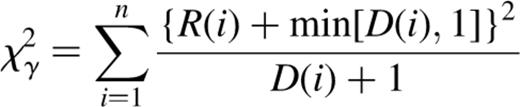
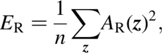
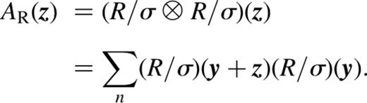
As PP92 showed, the expected value of E_R is equal to the number of lags included in the summation in equation (2.8), and the extent over which lag terms are useful is determined by the size of the instrumental psf. For the applications described below, an acceptable fit is defined to be one that has + the number of lag terms being considered. This is true ∼ 90 per cent of the time for normally distributed noise or Poisson-distributed noise when the mean signal is

To minimize the misfit statistic, the Polak–Ribiere conjugate gradient algorithm in Numerical Recipes (Press et al. 1992) was used. Some alterations were made to tailor the general purpose routine to this specific task, as detailed in Appendix A. In order to have non-negative inferred truths, PP92 suggested using transformed pseudo-image values, H_t, in the minimization where

(2.10)

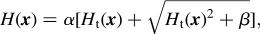
with and This transformation was used for the example in Section 3.1, but created a poor reconstruction of the low-signal regions in the examples in Section 3.2. For these cases, setting and simply truncating negative values yielded superior results without significantly affecting the speed of the code.

The calculation of the gradient of the misfit statistic with respect to the transformed pseudo-image values is a bit messy. After all, changing H_t, or effectively H, alters the inferred truth in surrounding pixels. This is then convolved with the instrumental psf before the residuals and hence the misfit are calculated. Appendix B contains the results of this calculation, but the important point is that it can be split up into correlations and convolutions.

3 Applications

The speedy pixon algorithm was applied to two simulated astronomical data sets. In the first case, the challenge of identifying galaxy clusters in cosmic microwave background (CMB) maps was considered for an instrument with specifications like those of the Planck surveyor. The formalism described above will be extended to deal with the multifrequency and multicomponent natures of the data and truth, respectively. In the second example some simulated ‘β’-profiles convolved with a large psf, such as the ASCA X-ray detector would measure when pointed at galaxy clusters, are reconstructed.

3.1 Multiwavelength cluster detection in simulated CMB data

The Planck surveyor satellite (Tauber, Pace & Volonté 1994) is expected to return maps of the sky in a number of microwave wavelength ranges. In addition to the intrinsic CMB fluctuations, a number of interesting foregrounds will also contribute to these maps. One such contribution will come from the Sunyaev–Zel'dovich (SZ) effect produced when CMB photons are inverse Compton scattered during their passage through the ionized gas in galaxy clusters (Sunyaev & Zel'dovich 1972). The distinctive spectral distortion created by the net heating of CMB photons in the directions of galaxy clusters should enable some thousands of clusters to be detected by Planck (Hobson et al. 1998).

3.1.1 Additional formalism

The formalism described here will assume that the spectral dependence of each of the components (i.e. CMB, SZ and noise) is known and constant over the region being observed, although in principle this could also be left as a part of the model over which the probability is maximized. For each of the n_c components, the spectral template will be denoted by where n is the number of wavebands in the observed data. Thus the inferred truth in waveband j can be written

(3.1)

Each component has its own pixon distribution and pseudo-image denoted by the c subscript. The pseudo-image variables for the intrinsic CMB and thermal SZ components are the thermodynamic ΔTT and the Comptonization parameter y, respectively, both in units of 10⁻⁶. Note that ΔTT can take positive or negative values so the transformed pseudo-image is chosen to equal the pseudo-image for this component, whereas equation (2.10) is used to ensure that H_SZ(x) (≡y) is non-negative in all pixels. For the reconstructions presented below, the value of ψ, as defined in equation (2.2), was set to zero such that all pixons were normalized to unity. In practice, it may be beneficial to allow ψ to be a function of component.

The multiwavelength data, and the fact that the CMB component can take positive or negative values, require a definition of pixon SNR differing from that in equation (2.5). This is chosen to be

(3.2)

The 1 index with the T̂ and σ² terms represents that only the first waveband is being used to define the SNR and δ_1,c is the smallest pixon width for component c. For the type of data simulated here, with the intrinsic CMB component dominating the thermal SZ component, it is possible, if the required pixon SNR is the same for all components, to find an acceptable fit to the data without the need for a cluster component in the inferred truth. In order to allow a better reconstruction of the weaker component (i.e. a reconstruction that includes some signal), it is necessary to introduce factors g_SNR(c) such that the actual pixon SNR requested for pixons representing component c is g_SNR(c) times the default value. While these factors could be left for the pixon algorithm to evaluate in a Bayesian fashion, this would be rather time consuming. In practice the relative strengths of the components were set to and 0.1 for the intrinsic CMB and thermal SZ components, respectively, in order that clusters were found, without introducing many spurious sources.

The υ parameter for determining the variation in pixon SNR across the image for a given component was set to 1 for both the CMB and SZ components. This enforced a flat pixon SNR across each of the component maps If some SNR variation was to be used, then an average over wavebands of the reduced residuals convolved with the local pixon shape would need to be calculated, rather than the monochromatic version contained in equation (2.6).

To deal with the sharp edge in the observed data, the reconstructed images were allowed to extend beyond the original data pixel grid. A total of 512² pixels were used and those lying outside the input data image had defined in them, but were otherwise treated identically with the rest of the reconstructed image pixels. This buffer region allows the pixon SNR to be sensibly defined, so that the inferred truths have the same sensitivity across all of the observed image while not directly influencing the calculation of the misfit statistic.

The computation of the misfit statistic includes n different residual maps and the definition of an acceptable value is modified accordingly. In addition, the misfit minimization is performed over variables.

3.1.2 Data production

A 400² pixel, 10 deg² field of simulated CMB sky, was created including both intrinsic CMB fluctuations and thermal SZ distortions produced by clusters, The intrinsic CMB map was a realization of the standard cold dark matter model using the power spectrum returned by cmbfast (Seljak & Zaldarriaga 1996). The thermal SZ map was produced by creating some templates from the hydrodynamical galaxy cluster simulations of Eke, Navarro & Frenk (1998) and then pasting these, suitably scaled, at random angular positions with mass and redshift distributions according to the Press–Schechter formalism (Press & Schechter 1974). The thermal SZ Comptonization parameter, y, and the thermodynamic ΔTT of the intrinsic CMB fluctuations were converted to fluxes per pixel in mJy¹ in each of four wavebands by multiplying by ω_c( j) as listed in columns 4 and 5 of Table 1. These four combined truths were then ‘observed’ by applying the relevant Gaussian beam and adding the pixel noise appropriate to each wavelength (see columns 2 and 3 of Table 1).

Table 1.

Lists of (1) the central Planck observing frequencies employed here (GHz); (2) the Gaussian full width half maxima (arcmin); (3) the 1s Gaussian noise per 1.5-arcmin² pixel in mJy (for 14 months of observations); (4) the conversion factor relating thermodynamic CMB ?TT, in units of 10⁻⁶, to the change in flux in mJy in a pixel; (5) the conversion factor relating the Comptonization parameter y, in units of 10⁻⁶, to the change in flux in mJy in a pixel; (6) the rms cluster T*B per pixel (mJy); (7) the maximum amplitude of cluster T*B per pixel (mJy); (8) the rms intrinsic CMB T*B per pixel (mJy); (9) the maximum amplitude of intrinsic CMB per pixel (mJy).

Open in new tabDownload slide

The final four columns in Table 1 show the maximum and rms per pixel produced by each of the two components separately. These numbers demonstrate both the high SNR with which Planck will observe the intrinsic CMB fluctuations and the relatively low SNR of even the brightest cluster in the field, after convolution with the instrumental psfs.

3.1.3 Results

The sets of pixon widths for the two components were chosen to be and For the intrinsic CMB, the SNR is so good that the pixons do not need to be very large before they prevent an acceptable fit from being found. In the SZ clusters case, the selection of a small and a very large pixon size allows the reconstruction of sharp features in a smooth background. The intermediate-sized pixon helps the pixons bridge the gap between background and cluster as the pixon SNR is reduced and the map becomes progressively less correlated. These SZ pixon widths are selected to match the scales of the features expected to be present for this component map. About 20 minutes of computer time were required to perform the multicomponent and multiwavelength speedy pixon reconstruction of the 400² pixel image (padded up to 512² pixels). For comparison a ML reconstruction with all pixons being set to be pixel-sized was also performed. This took approximately 3 min to complete.

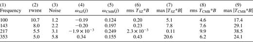
In Fig. 2, the pixon and ML-inferred truths for the intrinsic CMB flux at 100 GHz are compared with the true values in each pixel. The top panels show the distributions of reconstruction errors per pixel for the two methods, along with the widths of the best-fitting Gaussians for these distributions. Comparing the raw data (i.e. including SZ clusters, convolution with the beam and noise) with the true intrinsic CMB pixel values, leads to a best-fitting Gaussian width of 1.70 mJy, so it is apparent that both pixon and ML reconstructions have cleaned the data to some extent, although the narrowing of the error distribution is significantly better for the pixon case. The lower panels show trends for both the mean (full curves) and standard deviation (dotted curves) of the flux errors as a function of the true pixel flux. In the ML case, the scatter in the flux errors is large and approximately independent of the true signal, whereas for the pixon reconstruction the scatter is suppressed but increases when the signal is strong and the pixon width being used becomes smaller. Where the scatter in the error increases, the mean difference between the pixon-inferred and true signals decreases. This shows that for pixels with absolute values of intrinsic CMB 100-GHz flux exceeding ∼6 mJy, a smaller pixon width has been selected and the fit has improved. The choice of pixon widths is thus very important in determining these results. In the ML case, the trend in the mean error shows that the peak sizes are underestimated systematically.

Figure 2.

The top left-hand panel contains a histogram of the difference between the true and pixon-inferred intrinsic CMB component fluxes at 100 GHz in each pixel. Flux units are mJy for all panels in this figure. The width of the best-fitting Gaussian is also given. In the lower left-hand panel, the full curve represents the average difference between the true and pixon-inferred intrinsic CMB component fluxes as a function of the true pixel flux, and the dotted curve traces the standard deviation of the reconstruction error. The two right-hand panels show the corresponding results for the ML reconstruction. In both cases, the Gaussian fits to the reconstruction errors are not shown because they essentially lie on top of the histograms.

Open in new tabDownload slide

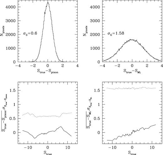
Fig. 3 is a grey-scale comparison of the true (top panel), ML-inferred (middle) and pixon-inferred (bottom) cluster y maps. It is very apparent that the pixon reconstruction has greatly suppressed the noise relative to the ML effort. There are a few sources in the pixon reconstruction that do not correspond with single identifiable sources in the actual truth. In regions where the density of small clusters is particularly high, the pixon algorithm has a tendency to place a single bright source to model the emission. However, relative to the ML effort, the compression of the reconstructed information is very clear. The pixon algorithm has essentially already made the decision as to which of the many ML sources are statistically justifiable. Reducing the SZ pixon SNR relative to that of the intrinsic CMB using the g_SNR(SZ) parameter would allow the pixon algorithm to detect clusters with smaller fluxes, albeit with an increased risk of producing spurious sources. The mean Compton y parameters per pixel in units of 10⁻⁶ are 0.80, 1.25 and 0.79 for the true, ML and pixon images, respectively, so the pixon algorithm does a good job of conserving the entire thermal SZ flux, in contrast to the ML technique.

Figure 3.

The true thermal SZ y map is shown in the top panel, and the ML and pixon-inferred truths are contained in the second and third panels, respectively. Axes are labelled in pixels.

Open in new tabDownload slide

As an aside, the inclusion of an intrinsic CMB component does not affect the cluster detection efficiency significantly. The important quantity is the SNR with which the clusters alone would be observed. Other foregrounds such as dust and Galactic free–free and synchrotron emissions are unlikely to vary on small scales and should not greatly affect the ability of the algorithm to detect clusters (see, e.g., Hobson et al. 1998).

3.2 Simulated ASCA X-ray cluster data with Poisson-distributed noise

X-ray imaging of galaxy clusters using the ASCA satellite involves convolution with a broad energy-dependent instrumental psf. The fact that the psf varies with position in the image will be neglected in the following examples, because equation (1.1) is inapplicable in such situations and, if the bulk of the emission is very concentrated then the instrumental psf will be approximately constant over the region of interest, in which case this treatment would be valid. ASCA has a particularly broad psf for an X-ray instrument, so its use for imaging might appear rather surprising. However, the good spectral resolution, coupled with the energy-dependence of the psf creates a situation where an image reconstruction algorithm could, for instance, be usefully employed in determining temperature maps of the ionized gas in X-ray clusters. Poisson, rather than Gaussian, noise is appropriate for these images where the number of photons per pixel is small.

3.2.1 Data production

Two different surface brightness profiles were created in a 256² pixel grid according to

(3.3)

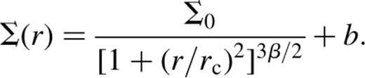
This is the β-profile proposed by Cavaliere & Fusco-Femiano (1976) to represent cluster X-ray surface brightness profiles with b corresponding to an additional background contribution. The high SNR model had 5 pixels, 0.7, 0.1 counts pixel⁻¹) whereas the low SNR truth used (7,6,0.7,0.001). These truths were chosen to be similar to what the ASCA satellite would have seen when looking at a cluster in the energy ranges and A non-circularly symmetric ASCA-like psf having a full width half maximum of ∼10 pixels was applied to these two truths and 10 Monte Carlo realizations of the resulting were made. After smearing out with the beam, the maximum count pixel⁻¹ were ∼70 and 1.5 for the two data sets, giving signal-to-noise ratios of and at the peak of the emission.

3.2.2 Results

Reconstructions were performed using 12 pixons ranging in size from to (separated by factors of ∼1.3), and These choices were kept the same for both the data sets. For the Poisson-distributed noise the expected amplitude of the noise in pixel x was set such that The comparison ML reconstructions were performed by setting all pixon widths across the pseudo-image to equal one pixel.

For the low SNR example, a tolerable fit according to could actually be obtained with a flat T̂. Only when the misfit statistic was changed to E_R was it necessary to insert a source into the inferred truth in order to produce a good fit. That is, the correlated residuals produced when a uniform T̂ was used to describe the weak source were sufficiently small that their amplitudes were statistically acceptable. However, the spatial correlation of the residuals did have the power to discriminate between this residual field and the anticipated noise.

Fig. 4 shows the central regions of the ‘X-ray cluster’ for the high SNR data. The top-left panel shows the truth, and one of the realizations of the observed data is shown beneath this. Both the smearing out of the sharply peaked emission and the introduction of noise are very evident. The pixon-inferred truth for this particular D is shown in the top-right panel and the corresponding ML-inferred truth is contained in the final panel. It can be seen that the noise is greatly suppressed by the pixon method and much of the peaked emission has been recovered on subpsf scales. The ML reconstruction also removes noise in the central regions, but at large radii spurious features are introduced, essentially fitting to the noise. Also, at small radii, the ML deconvolution does not do a good job of recovering the unsmeared profile.

Figure 4.

Contour plots for the X-ray cluster example in Section 3.2 showing the central region of the high SNR true β profile (top left), one noisy realization of it (lower left), a pixon-inferred truth (top right) and the ML-inferred truth (lower right). The contour levels are 0.5,1,3,10,30 (bold), 70,150 and 300 count pixel⁻¹ and the scales on the axes are numbers of pixels.

Open in new tabDownload slide

More detailed results concerning the radial surface brightness profiles are shown in Fig. 5, for both the high and low SNR data sets. The mean pixon-inferred profiles are drawn as dotted lines along with error bars showing the standard deviation of the individual Monte Carlo reconstructions. Long broken curves represent the corresponding ML quantities. It is apparent and reassuring, particularly for the high SNR data, that the pixon algorithm tends to produce similar profiles, independent of what noise realization has been used. The ML results show a significantly larger dispersion in the reconstructions arising from the different noise realizations. However, for the pixon reconstructions, the error bars are sufficiently small that the systematic deviations between the inferred and actual truths can be seen. These are produced by the lack of richness in the pixon description which leads to a preference for particular profiles. Nevertheless, it is encouraging that the speedy pixon algorithm can yield such results for two very different quality data sets. In addition, the suppression of noise is very effective, with no hint of any spurious sources being produced in any of the realizations even for the low SNR simulations, in contrast to the ML reconstructions.

Figure 5.

Azimuthally averaged profiles, showing the performance of the pixon (dotted curves) and ML (long-dashed curves) algorithms for reconstructing high (upper panel) and low SNR beta profiles. Error bars on the reconstructed results represent the standard deviation of 10 Monte Carlo realizations of the same truth. For clarity, the error bars for the ML results have been displaced 0.02 to the right. The full width half maximum of the beam is ∼10 pixels. Full and short-dashed curves represent the true β profiles and the data, respectively.

Open in new tabDownload slide

4 Conclusions

The details of a speedy pixon method for image reconstruction have been given. This algorithm is such that the treatment of 256² pixel images is possible using only a few minutes on a typical workstation. The application of the method to two types of simulated data sets shows its ability to detect sources in low SNR data without introducing spurious objects, in addition to deconvolving the instrumental psf. These results are a marked improvement over a simple ML reconstruction procedure which is applied in the data pixel grid and includes a uniform image prior term. A more detailed study of the ability of the pixon method to find clusters through their SZ distortion of CMB maps is in progress, including a comparison with MEM.

Acknowledgments

I would like to thank George Efstathiou for his helpful comments, including pointing out to me the existence of pixons, Rüdiger Kneissl for his CMB map and many useful discussions, David White for providing ASCA details and helpful suggestions, Shaun Cole for FFT assistance and Doug Burke, Ofer Lahav and Radek Stompor for general enlightenment. This work was carried out with the support of a PPARC postdoctoral fellowship.

References

Appendix

Appendix A: Conjugate gradient minimization details

The vast majority of the run time of the speedy pixon method is spent calculating the derivative of the misfit statistic with respect to the transformed pseudo-image values, H_t, and evaluating the inferred truth for a given H_t. A couple of simple changes to the Numerical Recipes line minimization routine, linmin, significantly reduce the number of function and derivative calls, and thus merit a mention here. (A more detailed discussion of some of these issues is contained at http://wol.ra.phy.cam.ac.uk/mackay/c/macopt/html.)

First, the default tolerance requested by linmin is ∼10³ times more stringent than need be for this application. Secondly, the initial guesses at bracketing the step size required to reach the function minimum along the chosen direction can be made more efficiently. Rather than keeping them fixed at 0 and 1, these sizes should reflect the fact that the different steps in parameter space are likely to have similar magnitudes. Thus the initially guessed step size should be inversely proportional to the modulus of the vector along which the step is to be taken. In addition, allowing these estimates to adapt to previous values also leads to a more rapid minimization. Tuning the routine along these lines leads to a speed up of about an order of magnitude for the examples considered in this paper.

Appendix B: Calculation of the misfit statistic derivatives

The conjugate gradient misfit statistic minimization requires the evaluation of the partial derivatives of the statistic (hereafter labelled μ) with respect to the transformed pseudo-image variables. The chain rule for differentiation gives

(B1)

Defining the partial derivative of μ with respect to by F(x), the derivative of μ with respect to the pseudo-image can be written as

(B2)

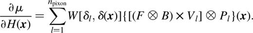
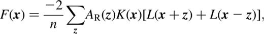
V_l represents a mask that is unity in pixels with and zero otherwise. The calculation can be seen to be a series of n_pixon correlations, hence the n log n scaling. F is readily shown to be −2R/(nσ²) and for χ² and respectively.

In the case of the autocorrelation of the residuals when the anticipated noise amplitude is independent of signal and position in the image (i.e. for the examples considered in Section 3.1), equation (B2) is still applicable, but the derivative of E_R with respect to needs to include a sum over lag terms:

(B3)

The sum of residuals comes from the derivative of A_R(z) with respect to R(x).

When the anticipated noise amplitude σ also depends upon the signal in the pixel, as is the case for the Poisson noise used in the examples in Section 3.2, the derivative calculation becomes somewhat more involved. Referring back to equation (B2), the required form for F becomes

(B4)

where

(B5)

and

(B6)