


Abstract
The data reduction process for optical emission-line observations of galaxies using the TAURUS-2 Fabry-Perot interferometer mounted on the 3.9-m Anglo-Australian Telescope is described in detail. The initial steps (bias subtraction, flat-fielding, etc.) are the same as for calibration of CCD images, and the wavelength calibration is similar to that in optical spectroscopy. The final steps are specific to Fabry-Perot instruments, and include the fitting of several instrumental parameters and a phase correction to convert the raw (x, y, z) data cube into a useful position-velocity (α, δ, v) cube. Software has been written to assist with the latter steps of the data reduction. Hα observations of NGC 1808, NGC 2442 and Circinus are used to demonstrate the reduction process.
1 Introduction
Although there is a large amount of literature available on the reduction and analysis of Fabry-Perot data taken with various instruments (e.g. Bland & Tully 1989; Atherton et al. 1982), it remains a difficult process for the non-expert user. With this general step-by-step guide we hope to facilitate future data reduction and analysis using new and existing software.
TAURUS-21 is a wide-field imaging Fabry-Perot interferometer designed to obtain narrow-band optical spectra. A comprehensive description of the instrument and its operation can be found in Taylor (1992), and some details in Bland-Hawthorn (1995). The main use of the TAURUS-2 instrument is to measure velocity fields of extended emission-line objects (e.g. galaxies and nebulae). The TAURUS-2 instrument is a descendant of the earlier TAURUS-1 described by Atherton et al. (1982), and is similar in principle and operation to Fabry-Perot instruments in use at a number of other observatories (for a summary see Bland & Tully 1989). For further reading, refer to Bland, Taylor & Atherton (1987), Lewis & Unger (1992), Shopbell, Bland-Hawthorn & Cecil (1992) and Sugai et al. (1994). The description here will mostly apply to any Fabry-Perot instrument. This paper describes in part observations that were made of the galaxies NGC 2442 (Houghton 1998), Circinus (Elmouttie et al. 1998), and particularly NGC 1808 (Koribalski et al., in preparation), which have been used as an example here, but are published in detail elsewhere.
2 The Instrument
The TAURUS-2 imaging Fabry-Perot interferometer was installed at the f/8 Cassegrain focus of the 3.9-m Anglo-Australian Telescope (AAT).
A detailed description of the major optical components is given in the AAO TAURUS-2 manual by Taylor (1992). The individual components used, in order along the light path, are the following:
- (i)
a ‘focal-plane’ filter, located slightly before the focal plane;
- (ii)
a ‘focal-plane’ aperture, located in the Cassegrain focal plane;
- (iii)
an iris;
- (iv)
a collimator (focal length fcoll = 473.9 mm);
- (v)
a ‘pupil-plane’ filter (not used here);
- (vi)
a Fabry-Perot etalon;
- (vii)
a camera (focal length fcam = 127.8 mm);
- (viii)
a Tektronix CCD detector.
The filter, the etalon and the detector are the most significant components for data reduction, and are described in detail.
2.1 The filter
The filter is used to select the appropriate wavelength range. It is usually an interference filter which works on a similar principle to the etalon (see below), but with a fixed glass plate instead of an adjustable air gap, giving a much larger passband for light, and a very broad interference pattern.
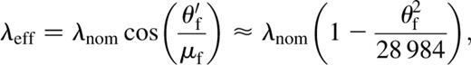
For the Hα observations of NGC 1808 we chose an R-band filter (6594/45) with a central wavelength of λnom = 6594 Å and a nominal bandpass of 45 Å. The filter can be tilted to an angle θf of up to 15° with respect to the optic axis, which effectively moves the central wavelength towards the blue end of the spectrum:
The original field size of the detector (∼10.2 arcmin) is restricted to about 5.5 arcmin by the 50-mm diameter of the filter. The scale at the input focal plane is 6.7 arcsec mm−1.
2.2 The etalon
A Fabry-Perot etalon (e.g. section 9.6 of Hecht 1987) consists of two transparent plates, usually made of glass, which are extremely smooth and are kept parallel and close together, generally separated by air. The distance between the plates (l) can be varied accurately under computer control to adjust the wavelength scale of the device. A partially reflective coating on the inside surfaces of the plates establishes an interference pattern between multiple reflections of incoming plane waves. To keep the refractive index of the air gap (μ) as stable as possible, the etalon cavity is continually flushed with dry nitrogen.
The etalon acts as a tunable interference filter, selecting particular wavelengths and attenuating others, depending on the angle (θ) of the incoming plane wave and the spacing between the plates.
The etalon itself is prone to ghost images owing to internal reflections in the TAURUS-2 instrument. These are removed by tilting the etalon slightly (see Bland & Tully 1989; Bland-Hawthorn & Taylor 1994).
We used a Queensgate ET70 etalon borrowed from the University of Maryland, which is one of the Taurus Tunable Filters (TTFs).2 This had a 70-mm aperture, an optical gap range of l≈40–44 μm (≈40 μm was used), an Hα free spectral range of Δλ≈54 Å, and a high finesse of N≈40. See Section 3.1 for definitions of these terms. The exact values need to be determined by fitting the observed calibration lines and instrumental parameters, respectively, during the data reduction process.
2.3 The detector
We used a 1024×1024 pixel Tek CCD as the detector.3 The readout noise (σR) and time (τR) are 2.3 e−1 and 60 s, respectively. The pixel size (p) is 24 μm. Using a scale of 24.84 arcsec mm−1 at the detector this corresponds to 0.596 arcsec. The focal length at the detector is fcam = 127.8 μm (≈5325 pixel).
3 Observations
During our run with the AAT TAURUS-2 instrument in 1995 February, three southern spiral galaxies were observed: NGC 1808, NGC 2442 and Circinus. Here we describe the observations of the source NGC 1808 as well as related calibration images and cubes. The analysis and interpretation of these galaxies are presented in three different papers (NGC 1808: Koribalski et al., in preparation; NGC 2442: Houghton 1998; Circinus: Elmouttie et al. 1998).
3.1 General information
Fabry-Perot observations are made by taking a succession of CCD (x, y) images of a source, such as a galaxy, with the etalon spacing parameter (z) set to a range of values. The etalon spacing is incremented by a constant amount from one image to the next to build up a three-dimensional (x, y, z) data cube. The distance between the etalon plates (l) has a linear relationship to the parameter z:
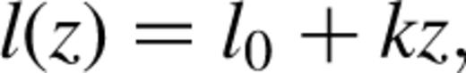
where l0 and k are constants defined by the gap control hardware.
The interference pattern produced by a Fabry-Perot etalon is a function of the following variables:
- (i)
R, the reflectivity of the etalon plate coatings;
- (ii)
μ, the refractive index of the gap;
- (iii)
λ, the observed wavelength;
- (iv)
θ, the angle from the optic axis, a function of position in the image, (x, y).
Here, ‘fixed θ’ and ‘fixed position’ are equivalent terms.
The reflectivity R is assumed constant, but may in fact vary slightly as a function of wavelength.
The mathematical analysis in this paper also assumes that μ is fixed, but l is variable. Some instruments vary the gas pressure (and hence μ) rather than varying l. This can be made mathematically equivalent (and so consistent with this paper), if l here is replaced with the ‘effective plate spacing’ (μl), and μ here is replaced with 1.
The monochromatic intensity response is given (e.g. Bland & Tully 1989) by the Airy function A:
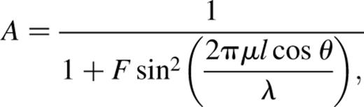
For a given position θ, the two variables are l and λ. Holding one of these fixed, while varying the other, produces a profile containing a number of peaks at points where constructive interference occurs, which meet the following condition:

For fixed λ and θ, equation (4) is satisfied by a series of equally spaced l values, one per n. Therefore the profile as l varies consists of a periodic series of relatively narrow and symmetrical peaks, interspersed with almost complete darkness.
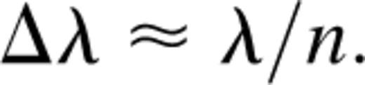
For fixed l and θ, a similar multipeak profile is produced as λ varies, with peaks for a number of wavelengths at different orders n. The full width at half-maximum (FWHM) of the peaks in the profile is defined to be the wavelength resolution, denoted here by δλ. The increase in wavelength λ that decreases n by exactly one, at the same l and θ, is defined to be the free spectral range (FSR), denoted by Δλ and given by the following:
The main practical effect of this ambiguity is that a given (x, y, z) position in a data cube could potentially contain emission from multiple wavelengths.
The figure of merit used to describe the wavelength resolution of the etalon is the finesse (N), a high value being desirable. N is given by the following (Bland & Tully 1989; section 9.6 of Hecht 1987):
For TAURUS-2 on the AAT, the available TTF etalons cover a range in zero-point gap of l0 = 15–500 μm, typical interference orders n = 45–2000, a range in FSR of Δλ = 2.5–250 Å, and a range in finesse of N = 12–70.
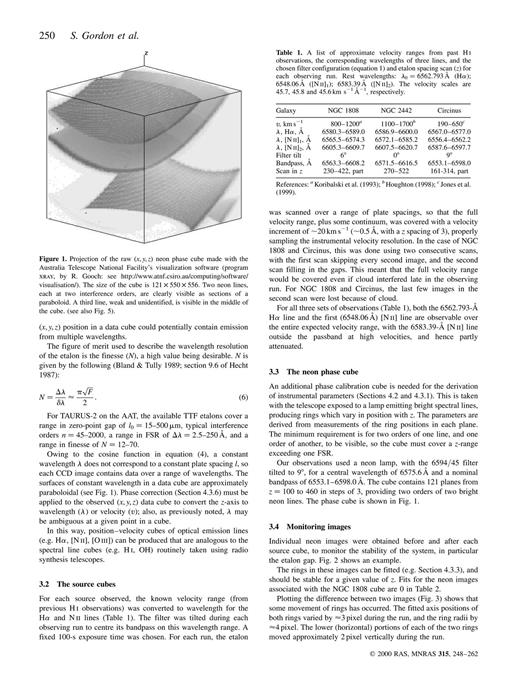
Owing to the cosine function in equation (4), a constant wavelength λ does not correspond to a constant plate spacing l, so each CCD image contains data over a range of wavelengths. The surfaces of constant wavelength in a data cube are approximately paraboloidal (see Fig. 1). Phase correction (Section 4.3.6) must be applied to the observed (x, y, z) data cube to convert the z-axis to wavelength (λ) or velocity (v); also, as previously noted, λ may be ambiguous at a given point in a cube.
Projection of the raw (x, y, z) neon phase cube made with the Australia Telescope National Facility's visualization software (program xray, by R. Gooch: see ). The size of the cube is 121×550×556. Two neon lines, each at two interference orders, are clearly visible as sections of a paraboloid. A third line, weak and unidentified, is visible in the middle of the cube. (see also Fig. 5).
In this way, position-velocity cubes of optical emission lines (e.g. Hα, [N ii], [O iii]) can be produced that are analogous to the spectral line cubes (e.g. H i, OH) routinely taken using radio synthesis telescopes.
3.2 The source cubes
For each source observed, the known velocity range (from previous H i observations) was converted to wavelength for the Hα and N ii lines (Table 1).1 The filter was tilted during each observing run to centre its bandpass on this wavelength range. A fixed 100-s exposure time was chosen. For each run, the etalon was scanned over a range of plate spacings, so that the full velocity range, plus some continuum, was covered with a velocity increment of ∼20 km s−1 (∼0.5 Å, with a z spacing of 3), properly sampling the instrumental velocity resolution. In the case of NGC 1808 and Circinus, this was done using two consecutive scans, with the first scan skipping every second image, and the second scan filling in the gaps. This meant that the full velocity range would be covered even if cloud interfered late in the observing run. For NGC 1808 and Circinus, the last few images in the second scan were lost because of cloud.
![A list of approximate velocity ranges from past H i observations, the corresponding wavelengths of three lines, and the chosen filter configuration (equation 1) and etalon spacing scan (z) for each observing run. Rest wavelengths: λ0 = 6562.793 Å (Hα); 6548.06 Å ([N ii]1); 6583.39 Å ([N ii]2). The velocity scales are 45.7, 45.8 and 45.6 km s−1 Å−1, respectively.](https://oup.silverchair-cdn.com/oup/backfile/Content_public/Journal/mnras/315/2/10.1046/j.1365-8711.2000.03348.x/2/m_315-2-248-tbl001.jpeg?Expires=1750295201&Signature=lBud3GCeSjFGRdTONeDA-QrE3a5R0xg2zYJ19pdA~V9OM~p7TXXhptxVigOfBKb9VuGCYiGoflVLxaezB2Xz2lvzt61LuDwRFo-dv92wEdAdq7NcW-FYIVBLUudvezO0e5jS4rvKihhWda~Znjc0-0szXkYhxBzKnuQBQcsxvr4IxGMZBtNOXGnb4uGlrY8R7n-d2k44rC888uSNVdQ84uefP~nw-PdXEMFy7reX-JssJKEHBYh6kR9V41jTlT2CPoA3g9wTOzimhrMzXUTkXvSpTOwJm4rWWZc8cGMK~BNMMejFXPk1Sn-T58OUdqrL1j8A6voj7YjhYp~Mi3P3bA__&Key-Pair-Id=APKAIE5G5CRDK6RD3PGA)
A list of approximate velocity ranges from past H i observations, the corresponding wavelengths of three lines, and the chosen filter configuration (equation 1) and etalon spacing scan (z) for each observing run. Rest wavelengths: λ0 = 6562.793 Å (Hα); 6548.06 Å ([N ii]1); 6583.39 Å ([N ii]2). The velocity scales are 45.7, 45.8 and 45.6 km s−1 Å−1, respectively.
For all three sets of observations (Table 1), both the 6562.793-Å Hα line and the first (6548.06 Å) [N ii] line are observable over the entire expected velocity range, with the 6583.39-Å [N ii] line outside the passband at high velocities, and hence partly attenuated.
3.3 The neon phase cube
An additional phase calibration cube is needed for the derivation of instrumental parameters (Sections 4.2 and 4.3.1). This is taken with the telescope exposed to a lamp emitting bright spectral lines, producing rings which vary in position with z. The parameters are derived from measurements of the ring positions in each plane. The minimum requirement is for two orders of one line, and one order of another, to be visible, so the cube must cover a z-range exceeding one FSR.
Our observations used a neon lamp, with the 6594/45 filter tilted to 9°, for a central wavelength of 6575.6 Å and a nominal bandpass of 6553.1–6598.0 Å. The cube contains 121 planes from z = 100 to 460 in steps of 3, providing two orders of two bright neon lines. The phase cube is shown in Fig. 1.
3.4 Monitoring images
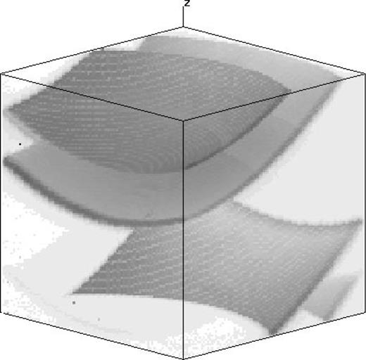
Individual neon images were obtained before and after each source cube, to monitor the stability of the system, in particular the etalon gap. Fig. 2 shows an example.
The neon stability monitoring image taken with the TAURUS-2 instrument immediately after the NGC 1808 cube (exposure time 2 s; etalon gap z = 100). The image is 550×556 pixel, with the bias columns visible along the right-hand edge. Bias and flat-field correction have been performed (Section 4.1.2).
The rings in these images can be fitted (e.g. Section 4.3.3), and should be stable for a given value of z. Fits for the neon images associated with the NGC 1808 cube are 0 in Table 2.2
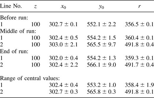
Ring centre (x0, y0) and radius (r) for the two identified neon lines in the stability monitoring images taken during the NGC 1808 run, using the program fpring. Uncertainties indicate scatter in the fit. Also given is the range of values (mean±d;d;difference).
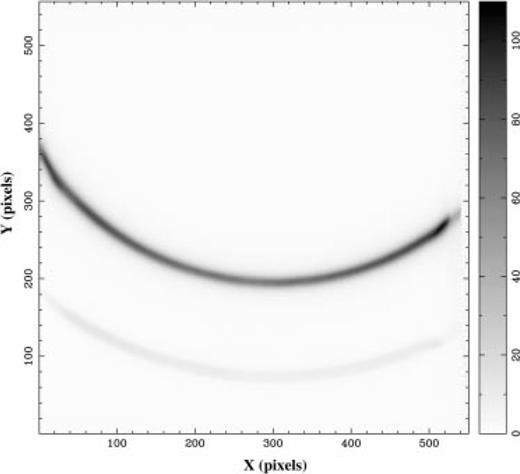
Plotting the difference between two images (Fig. 3) shows that some movement of rings has occurred. The fitted axis positions of both rings varied by ≈3 pixel during the run, and the ring radii by ≈4 pixel. The lower (horizontal) portions of each of the two rings moved approximately 2 pixel vertically during the run.
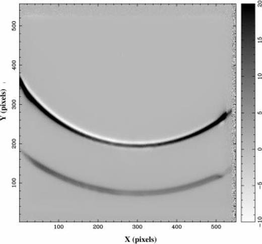
The difference between neon monitoring images before and after the NGC 1808 run, showing movement of the rings.
Ring 1 (the smaller and brighter one) gave tighter and more consistent ring fits than did ring 2. Ring 2 also gave a fitted axis position deviating from the established position (x0,y0)∼(303,554), indicating distortion. Distortion is also suggested by the large radius of ring 2, which places it in the vignetted regions of the image. These and the low brightness of the ring indicate that ring 1 gives a more accurate indication of stability.
The stability during the NGC 1808 data cube is thus expected to be comparable to that of ring 1, ∼3 pixel≈1.8 arcsec in (x0,y0) and ∼4 pixel≈2.4 arcsec in r. Ideally it would be desirable to estimate how position and radius vary over time, to allow a correction to be applied; however, with only the three monitoring images taken, this is not achievable in this case.
3.5 The white light cube
Overall, the Fabry-Perot instrument has a response to light (apart from the Airy pattern) which varies with both wavelength and position in the image (spatial dependence). These variations can both be quite major, and certainly need to be corrected for as a part of the calibration, to avoid distortions and poor flux calibration.
The wavelength dependence results mainly from the overall spectral response of the following:
- (i)
the blocking filters, e.g. focal and pupil plane;
- (ii)
the etalon (additional to the Airy pattern);
- (iii)
the detector (usually a CCD).
The spatial dependence results mainly from the following:
- (i)
the aperture size and shape of filters and the etalon, i.e. vignetting effects;
- (ii)
varying sensitivities between different CCD pixels, e.g. owing to manufacturing variations.
These responses generally do not vary during an observing run, so the overall response is measured using a separate three-dimensional flat-field image known as a white light (or WL) cube. This is obtained by flooding the telescope with uniform white light from a lamp, and scanning the etalon through a range of spacings to obtain a Fabry-Perot data cube. The range of spacings is chosen to match exactly those of the on-source cube(s) needing correction.
The spatial response is shown clearly in Fig. 4, which is an average of all planes of the WL cube for NGC 1808. This was obtained using a tungsten lamp. The sensitivity drops markedly towards the edges of the image, and is enhanced in a region along the bottom, in addition to small-scale variations.
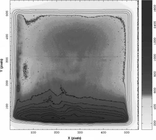
Average image 1obtained from the WL cube for the NGC 1808 run. Contours are 100, 200, 300, …, 800, 900, 1000, 1200, 1400, 1600 counts. The grey-scale uses histogram equalization from 120 to 1600 counts.
The resulting WL cube, being the numerical product of the wavelength and spatial dependences of the instrument, is used to correct an on-source cube for these effects in one operation, by dividing the on-source cube by the corresponding WL cube. Alternatively, appropriate averaging along cube axes can be used to map spatial and spectral response functions (not done here).
3.6 Reference star
Flat-field correction of CCD images (Section 4.1.2) produces a uniform flux scale for images, but not an absolute calibration of this scale, i.e. the conversion from CCD ‘counts’ to intensity. To provide this, observations are made of a non-variable reference star with a well-measured brightness. In our case, reference star LTT 3218 was observed at etalon spacings z = 100, 200 and 300, with the same 100-s exposure time used for on-source cubes. The position of the star is given in Hamuy et al. (1992) as J2000 RA = 08h41m33 6, Dec.=−32°56′55″, with a proper motion in RA and Dec. of μ = −1.26 arcsec yr−1, μ = 1.31 arcsec yr−1. Our observed position for the star in 1995 February was J2000 RA = 08h41m33
 2, Dec.=−32°56′52″, a displacement of Δα = −5 arcsec, Δδ = 3 arcsec, roughly corresponding to 4 years of proper motion.
4 Data Reduction
Data reduction for all Fabry-Perot instruments is rather involved, owing mainly to the enormous number of data contained in the cubes (source cube, WL cube, Ne cube) and the inherent complexity of the Airy interference pattern. The preliminary steps dealing with flat-fielding and calibration are common to most CCD observations. These can be performed readily with existing astronomical software such as aips4 and miriad,5 typically used for radio interferometer data, or midas6 and iraf7 used for CCD images and optical/infrared spectroscopy.
However, while some current free software (e.g. iraf) can do the phase correction of Fabry-Perot observations, these programs are not applicable for the results we desire. This is mainly because (1) the Airy rings in phase calibration images are incomplete owing to the axis being shifted off-centre, (2) the rings are distorted owing to flat-fielding not perfectly removing the uneven instrumental/CCD response, which defeats many ring-fitting algorithms, and (3) we desire to obtain spectral data cubes (with planes sampled at particular velocities), rather than only ‘moment’ maps as provided by some software.
In this section we describe a step-by-step data reduction method using a combination of aips or miriad, and a set of new Fabry-Perot tasks written by one of us (SG), which overcome these difficulties. The NGC 1808 data are used as an example.
Appendix A contains a brief guide to the reduction procedure.
4.1 CCD reduction
4.1.1 Bias subtraction
The electronics that read the CCD introduce a ‘bias’, which is a constant offset added to the value of every pixel as it is scanned out of the CCD array and digitized, regardless of exposure time or photon counts. The rightmost 10 columns of each image taken with the AAT and Tek CCD are not exposed to light, and thus measure the bias (see Fig. 2). We obtained a bias level for each plane by averaging the unexposed pixels. Since the bias varied only slightly within a cube, probably as a result of noise, a mean value was subtracted from all planes in the same cube.
The mean biases obtained from the NGC 1808 source cube and the corresponding white light cube were 101.1±0.6 and 102.0±0.6, respectively. A bias of 101.4±2.1 was found for the neon phase cube.
4.1.2 Flat-fielding
The response of the CCD to light varies from pixel to pixel, and distortions caused by the optics of the instrument produce marked intensity variations from one region to another of the image. In the case of our observations, the images have a fall-off in intensity towards all sides, and a marked brightening in the lower portion of the image. In order to correct for the response function of the instrument, each plane in the source cube was divided by the white light cube plane for the same z-value, after subtracting the bias level from each. In the case of the neon cube and monitoring images, where the z-value was not sampled by the white light cube, an average white light image was used instead (see e.g. Fig. 4), which involves some distortions but appears unavoidable. In some cases the white light cube may need to be smoothed spatially before the division, owing to small-scale variations within the cube (Bland et al. 1987).
This procedure is standard for the calibration of CCD images and is known as flat-fielding. See also Atherton et al. (1982).
4.1.3 Seeing correction and cosmic ray removal
All planes in each source cube need to be convolved with a Gaussian function corresponding to the worst seeing, so that the resulting images have a consistent and well-defined resolution throughout. Since seeing is an effect produced by passage through the atmosphere, it occurs before the light enters the telescope and instrumental response is not involved, and hence the convolution should be done after flat-fielding of the image.
Additionally, CCD images typically contain bright points or tracks produced by cosmic rays, which need to be removed prior to convolution to avoid contaminating the phase-corrected images. The removal process may be tedious, involving selectively masking out each ray in each image. The extent of this problem will depend on the brightness of the cosmic rays, and on the exposure times (more tracks in longer exposures). In some cases the cosmic ray removal is not necessary: for example, with the TAURUS-2 data described here, no masking was needed.
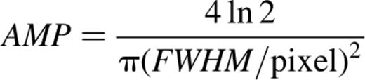
To perform convolution for the NGC 1808 data, two unsaturated stars both fitted Gaussians of FWHM≈1.8 arcsec (3 pixels), which we estimated to be the seeing for these observations. The fitting was performed using miriad task imfit, and the seeing correction using miriad task convol, with a FWHM of 1.8 arcsec and a ‘scale’ parameter [= Gaussian amplitude, equation (7)] of ∼0.0981 to preserve the intensity scale:
4.1.4 Flux calibration
This section establishes a calibration scale for converting fluxes measured in CCD counts into photometric units (i.e. in terms of energy). It should be noted that the observations used here were intended mainly for kinematic studies. Hence, while the following is correct to first order, some photometric corrections are absent. These particularly deal with the implications of filter bandpass and etalon FSR and resolution, which tend to alter the flux scale to some degree. Also, sky transparency variations which affect the flux scale for individual image frames have been omitted. These corrections need to be considered for accurate photometry.
The absolute flux calibration is derived from the images taken of star LTT 3218 (Section 3.6), using catalogued intensity measurements of that star as a reference (Stone & Baldwin 1983; Hamuy et al. 1992). The integrated CCD count for the stellar image, was 2503, 1595 and 2385 for z = 100, 200 and 300 respectively, after flat-fielding against a mean WL image (Fig. 4). The corresponding WL cube was the NGC 1808 one, which does not cover a full FSR, so only the z = 300 image was in the z-range of that cube, and neither of the other images was one FSR away from a covered value. Plane-to-plane variations in the flat-field response at the position of the star are up to ±8 per cent in the z-range covered, and could be much more outside that range, although there is no way to test this. It is thus necessary to use an average image for flat-fielding LTT 3218, introducing an unavoidable calibration error and possibly accounting for the differences between the three integrated counts. To minimize this possibility, the z = 200 image was dropped and an average of the remaining two used for calibration.
The catalogued flux density of the star interpolated for the central wavelength (λ = 6586 Å) is ∼5.17×10⁻²⁵ erg cm−2 s−1 Hz−1 or 12.13±0.004 mag according to Hamuy et al. (1992), and ∼5.82×10⁻²⁵ erg cm−2 s−1 Hz−1 or 11.99±0.09 mag according to Stone & Baldwin (1983). Using an average of the z = 100 and z = 300 counts gives absolute flux density scales of 2.115×10⁻²⁸ and 2.381×10⁻²⁸ erg cm−2 s−1 count−1 Hz−1 for the 100-s exposure flat-fielded images, with the two published flux densities. Using the conversion factor for Hα velocities,  gives equivalent scales of 3.201×10⁻¹⁹ and 3.604×10⁻¹⁹ erg cm−2 s−1 count−1 (km s−1)−1 for Hα line data. The ∼13 per cent difference between the two published flux densities represents another uncertainty in calibration.
To test this scale, the Hα flux of the inner 20×10 arcsec2 of the nuclear region of NGC 1808 was measured from the phase-corrected zeroth-moment map, as 2.85×10⁻¹² and 3.21×10⁻¹² erg cm−2 s−1 using the two scales, whereas Véron-Cetty & Véron (1985) measured this as 2.2×10⁻¹² erg cm−2 s−1, and Osmer, Smith & Weedman (1974) obtained 2.6×10⁻¹² erg cm−2 s−1. However, this region does not include the whole central Hα -emitting region, and the boundaries of the previous 20×10 arcsec2 region were not clearly defined in the Véron-Cetty & Véron paper. These measurements imply that our flux calibration is out by ∼10–20 per cent, which is reasonable given the uncertainties in its derivation, and the lack of spectral resolution and bandpass considerations. Alternatively, the NGC 1808 nucleus could be time-variable, which we cannot confirm or reject.
4.2 Wavelength calibration
The phase calibration cube needs to be studied to determine the wavelengths and orders of the calibration lines. This is referred to as ‘wavelength calibration’, since it establishes the wavelength scale for the data. Since it also establishes the velocity scale for any Doppler-shifted spectral lines that are later phase corrected, it is also by implication a ‘velocity calibration’. The conversion between the two variables is the standard Doppler relation, and is not described further here.
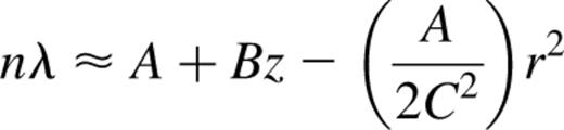
The emission lines in the neon phase cube (Fig. 1) are seen as surfaces of constant n and λ (see equation 4). The wavelengths of the neon lines closest to the central wavelength of the bandpass (see Section 3.3) are 6532.8824 and 6598.9528 Å (page E-209 in Weast 1975). These were identified by applying the following equations and process to spectra taken from the cube (Fig. 5).
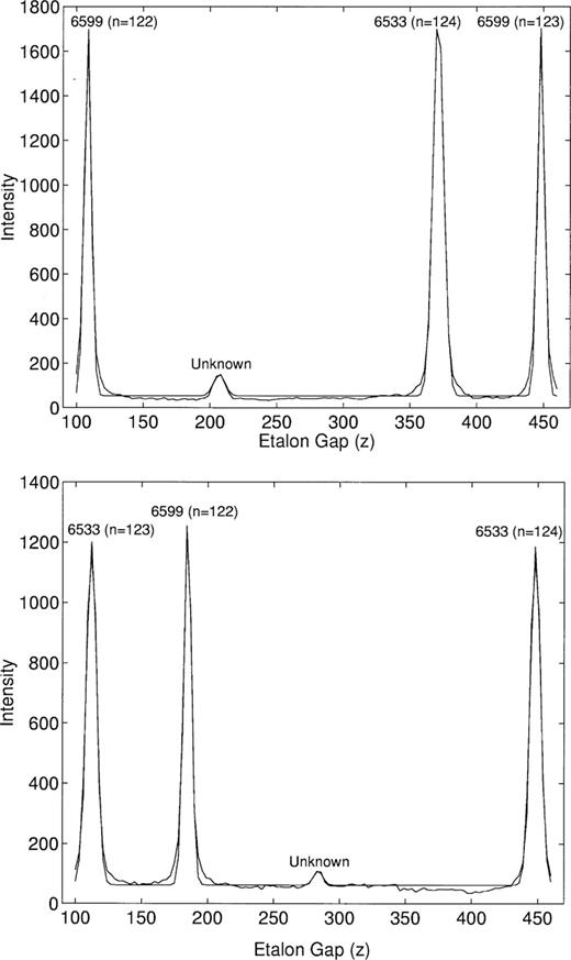
Two spectra through different (x,y) positions in the neon phase cube, overlaid with fits to four Gaussians plus a constant, using miriad tasks imsub and itemize and matlab function fmins. Peaks are as indicated (wavelength in Å and order in brackets). The left- and rightmost peaks in each case are from the same line. Their spacings are Δz1 = 336.2 for λ1 = 6532.8824 Å (bottom) and Δz2 = 339.4 for λ2 = 6598.9529 Å (top).

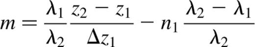
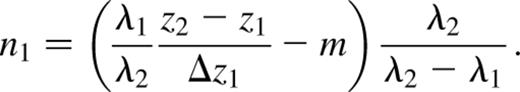
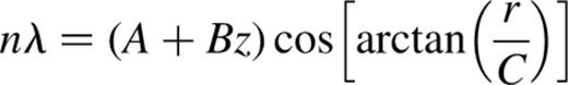
Given observations at a specific value of θ, of two spectral lines with wavelengths λ1 and λ2, with one order of each at (nn1, zz1) and (nn2, zz2) respectively, and also with the next higher order of λ1 displaced to zz1+Δz1, it is possible to transform equation (8) into the following which do not mention any instrumental parameters (where mn2−n1):
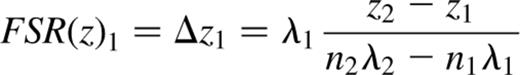
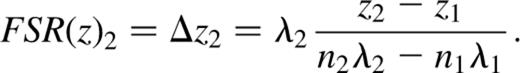
By slightly changing equation (10) we can calculate the FSR in z, FSR(z), for each wavelength:
To derive values for λ, n1 and n2, a profile is taken along the z-axis of the phase calibration cube at a particular (x, y) position (Fig. 5), and a fit made to the z-positions of each emission peak [one (n, λ) combination]. These fitted positions are inserted into equations (9) and (10) for various choices of λ and n1 or m, to find viable sets of values. The constraints are that n1 and n2 must be positive integers (hence also m is an integer); and that nλ must be ∼2l0 for the etalon.
Note that, in general, m depends on the lines being observed, and the range of z-values observed, and is not guaranteed to have any particular value, although it is typically almost zero For example, swapping the two spectral lines will change its sign. Thus the equations given here cannot be simplified in general to eliminate m.
Generally the filter bandpass is a small fraction of the central wavelength, so the fitted lines are of similar wavelength. Thus n1 in equation (10) is quite sensitive to errors in m, and m is well constrained. However, m in equation (9) is relatively insensitive to errors in n1, and n1 is poorly constrained. The overall effect is that generally the difference between order numbers is accurately determined, but they contain some consistent offset from their true values. Repeating the process for additional profiles may resolve uncertainties.
The peak positions can be found, e.g., using the slfit task in aips, or the fmins function in matlab with an appropriate model function. In the case of our observations, the resulting fit (summarized in Table 33) uniquely defined the differences between orders, but there is a possible offset of up to ±2, which was unavoidable. The quoted orders were the closest fit, which also gave the smallest residuals when deriving A, B and C later. We found that there were three different emission lines: the two strong ones are neon lines, λ1 = 6532.8824 Å and λ2 = 6598.9529 Å. The third line is very weak and has not been identified. The filter is obviously leaking, as the 6533-Å line gets through strongly even though it is outside the nominal passband.
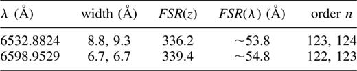
Calculated wavelengths, orders and FSR, by both definitions, of the calibration lines. n is uncertain by ∼±2, but differences between quoted orders are exact.
4.3 Phase correction
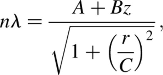
Phase correction is the conversion of the z-axis of the observed data cube to a wavelength (λ) or velocity (v) axis using equation (13). This transforms the paraboloidal surfaces for each order and wavelength into planes.
This section is an explanation of the following stages (in order) through which the observed data must pass to achieve phase correction.
- (i)
Find a parametric fit to the positions of peaks in the Airy function for the etalon, equation (3), in terms of z, λ and θ. This is a fitting exercise involving the following: determining n and λ for the calibration lines (already described in Section 4.2); measuring calibration ring positions and sizes (Section 4.3.3); averaging the ring centre positions to find the optic axis; and fitting a model equation to the ring sizes (Section 4.3.4). Note that this stage only needs be carried out once for each observation.
- (ii)
Determine the desired velocity or wavelength grid to be used (Section 4.3.5).
- (iii)
Correct the source data cube to produce a cube in v or λ (Section 4.3.6).
This description is mainly given in terms of software that we have written to carry out these stages, and how it functions. However, the stages described here are generally applicable.
Section 4.3.7 also describes the various artefacts of phase correction which may occur from time to time.
4.3.1 Determining instrumental parameters
The best-fitting values for the constants A, B, C, x0 and y0 are derived from the neon calibration cube. We used the new program fpring (Section 4.3.3) to derive (x0,y0) as well as a table containing z and r(z). The fpcal task (Section 4.3.4) was then used to perform a least-squares fit for the remaining constants A, B and C using z and r(z) from these tables. Since ring positions are not measured precisely, to constrain the fit it is necessary to use large numbers of rings for the fit, and for these to come from multiple spectral lines and orders so that nλ is not constant. For our observations, measurements of a total of 131 rings, from two orders of each neon line, were used. These results are summarized in Table 4.4
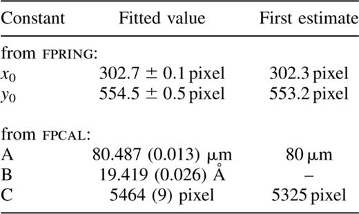
The best fit to constants in equation (13) determined with the fpring and fpcal tasks. The numbers in brackets are the approximate fit standard deviations in the same units. There were 131 samples (ring measurements in the fit). Residuals in nλ ranged up to 0.3 μm.
4.3.2 Fabry-Perot software
One software package that was evaluated was the iraf fabry package, produced by the Cerro Tololo Interamerican Observatory (CTIO) and originally written by George Jacoby.8 Although in general very useful, we found that several tasks were not adequate for our purposes. For example, the program ringpars requires entire interference rings to calculate the position of the optic axis, whereas in the TAURUS-2 data only partial rings are visible owing to a tilted etalon and a limited field of view (see Fig. 2). The fitring task in the same package had no such limitations, and a ported version (see below) was used to find the A, B and C constants.
Given our background mostly in radio astronomy, and the existence of standard astronomical software tailored to those needs, we decided to complement the existing software with a set of new programs, written as tasks for the miriad system (Sault, Teuben & Wright 1995). Unlike standard miriad tasks, they also support reading and writing of FITS images, and so can be recompiled as stand-alone programs with a command-line interface for users not having access to miriad. It is proposed to supply these tasks as an optional component of miriad distributions; however, this has not yet been implemented. The new programs are the following:
- (i)
fpring which locates the size and position of partial interference rings, given a rough estimate of the position supplied by the user;
- (ii)
fpcal which is a miriad port of the iraffitring task;
- (iii)
fprange which calculates the available velocity or wavelength range of a Fabry-Perot data cube, given the derived instrumental parameters and the rest wavelength of the spectral line of interest; it is useful for deciding on a velocity axis for phase correction;
- (iv)
fpcorr which carries out phase correction of a data cube, given the relevant instrumental parameters derived from a phase calibration cube;
- (v)
fpfake which produces simulated phase calibration images for a given set of instrumental parameters, allowing a comparison with the images from which the parameters were derived, as a test for fitting errors.
These tasks, with the exception of fpfake, are described in the following sections.
We would like to add that a new iraf package for the processing of Fabry-Perot data has been under development for some time (e.g. Bland-Hawthorn, Shopbell & Cecil 1992; Shopbell, Bland-Hawthorn & Cecil 1993). When completed, this package will be capable of, e.g., locating and parametrizing partial, elliptical interference rings and performing phase correction.
4.3.3 fpring: fit interference rings
In general, the program fpring can be used to determine the centre and radius of full or partial rings in an image, assuming that the rings are circular and of sufficient intensity, with a symmetrical profile so that the peak is at its centre. The fpring program is suitable for stable Fabry-Perot instruments such as TAURUS-2 on the AAT. This program serves the same role as the iraf task ringpars, but it has the added capability of fitting partial, circular rings as required by the TAURUS-2 data.
Note that, because of the details of the algorithms used, the program could well fail to fit rings from some instruments, particularly in the case of distorted rings or non-symmetric ring profiles.
The program locates the arc of the ring at one position in the image, and then traces changes in the position of the intensity peak, while examining successive positions advanced along either the x- or y-axis of the image (depending on direction from the ring centre). With this method, the ring needs to be continuous in the region being fitted, but it does not need to be a complete circle.
In this particular application, fpring is used to fit the centre (x0, y0) and radius (r) of particular interference rings in every plane (z) of the calibration cube. The program is run once for each interference ring or surface in the data cube. The results of each run are written into an ASCII table together with an estimate of the scatter in the radius measurement (see Table 5). 5 The scatter estimate can be used to remove bad fits. Large errors in the calculated quantities indicate that the ring is not circular, or too weak or too small to fit accurately.
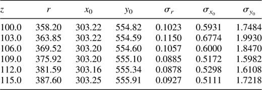
A partial listing of an fit output file from task fpring, showing the positions of one ring in the neon cube (6599 Å, n = 122) (Fig. 5), on a plane-by-plane basis. σ indicates ‘scatter’ between the fitted points on the rings, rather than an error margin.
The program requires the following interactive input parameters:
- (i)
input image file name;
- (ii)
z-start and z-step;
- (iii)
(optionally) a rectangular bounding box (in pixels) for a particular ring; to avoid confusion between the various rings, the calibration cube should be examined visually to define the region in which a particular interference ring is found;
- (iv)
output file name, in one of a number of formats.
4.3.4 fpcal: fit instrumental parameters
Given a list of the sizes and positions of rings as a function of z, it is necessary to fit these to the instrumental response function, equation (13). This is typically done using a least-squares fit. It is possible to do this either by approximating equation (13) to a parabolic one involving z and r, or by solving it directly using a non-linear regression algorithm.
Several software packages are already capable of this: e.g. the curve-fitting routines in matlab; lfit in Numerical Recipes (Press et al. 1992); and fitring in the CTIO Fabry-Perot package for iraf.
We opted to carry out this task by porting the existing iraf task fitring to the miriad environment, and slightly modifying the input format to match the output from fpring. The resulting task, called fpcal, performs a simple one-dimensional fit, ignoring the spatial structure in the Airy interference pattern (see Section 3.1).
The task does not, however, calculate residual maps showing misalignment between the calibration rings and the parameter fit obtained for the instrument.
fpcal takes as input the names of the input text files produced for each calibration line by fpring, along with the wavelength (λ) and order (n) of the line. It then performs an iterative non-linear least-squares fit to the A, B and C parameters in equation (13).
This task directly produces a summary of the residuals in the fit, for each ring listed, and the values of A, B and C with standard deviation error estimates. The task also supports interactive flagging of individual ring samples in the data, redoing the fit each time, which was not supported by fitring. This is generally used to remove samples producing large fit residuals, which indicate bad samples.
The resulting values for our TAURUS measurements and the optic axis position used are presented in Table 4.
4.3.5 fprange: velocity coverage
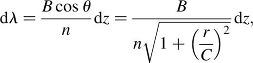
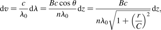
The program fprange can determine the velocity or wavelength range covered by a given data cube (not phase-corrected), given the instrumental parameters that will be used for phase correction, and for Doppler velocities the rest wavelength of the spectral line. This is useful for finding the velocity range covered by a cube, before doing phase correction.
This search can be constrained in λ to mimic a filter passband, or in order n, as well as spatially in (x,y). Since the wavelength range varies with position, the results are given as a range at the minimum and maximum distances r from the optic axis. Equation (14) is inverted for particular n and extreme z and r, to find λ (or v). The z-spacing of a cube (dz) is also converted into the corresponding wavelength or optical velocity resolution after phase correction (dλ or dv) using the following equations:
4.3.6 fpcorr: phase correction
The program fpcorr has been written to carry out phase correction, for a specified spectral line, given the fitted parameters A, B, C, x0 and y0.
Phase correction takes an on-source image cube as (x, y, z), and re-samples it along the z-axis to produce a second data cube with velocity, (x, y, v), or wavelength, (x, y, λ), as the third axis. The resampled column at a given (x, y) position depends only on the input column at the same (x, y) position.
Note that this process works in terms of wavelength, since this is the quantity relevant to the instrumental equations. Velocity for spectral lines is implemented by converting velocity to wavelength before performing resampling. One of the natural results of this (common to all phase correction techniques) is that, apart from the spectral line of interest, any other lines present in the input data will also be visible in the output map, but shifted to some (wrong) velocity position, if the velocity range sampled is wide enough. Likewise, continuum is carried through to the output unaltered. By way of example, Fig. 6 (top panel) shows [N ii] emission as well as Hα emission, before phase correction. This appears as faint arcs above the brighter Hα on the left-hand side of the nucleus, and below it on the right-hand side of the nucleus. Fig. 6 (bottom panel) shows that the continuum emission from the nucleus is present in all channels after phase correction.
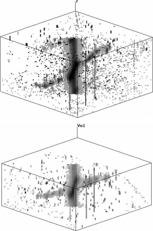
Projections of the NGC 1808 source cube (top panel) before and (bottom panel) after the phase correction process. Continuum has not been subtracted. The cubes have been reduced in spatial resolution by factors of 4 and 5, respectively. The phase-corrected data were derived using order n = 121 in equation (13). The phase-corrected cube covers velocities 620–1440 km s−1 (bottom to top).
To perform the resampling, the three-dimensional coordinates of each output pixel, (x, y, λ) or (x, y, v), are mapped to a corresponding set of coordinates, (x, y, z) in the input cube. This is done by converting (x, y) to a ring radius r, based on the optic axis position (x0, y0), then inverting equation (13) to find the value of z, and finally extracting the adjacent input pixels and interpolating to derive an output pixel value.
The input to the program consists of the following.
- (i)
The fitted instrumental parameters: A, B, C, x0 and y0 (calculated by fpring and fpcal).
- (ii)
The rest wavelength of the spectral line, if making a velocity cube, for example Hα or [N ii].
- (iii)
The names of one or more input images, containing images of the source, taken through the etalon for one z-setting or a series of them (as a cube). The usual RA, Dec. coordinates are along two spatial axes (x, y), with the z-value encoded as a non-spatial axis. An axis order of (z, x, y) or (x, z, y) is much faster owing to the specific implementation used, which, for efficiency of file access, resamples each spatial position as one operation.
- (iv)
The range, increment and type of the non-spatial axis, which can be in optical or radio velocity, wavelength or frequency. A further option, designed for testing fitted parameters against the phase calibration cube, ‘straightens out’ phase calibration cubes so that each line + order becomes a plane in the output.
- (v)
An optional rectangular spatial bounding box, to extract only a portion of the images (which speeds things up if used).
Note that the program does not attempt to correct for time variation in the instrumental parameters during observations, for example shifting of the optic axis. It also does not allow for the specification of a residual or phase map which would correct for deviations from the model instrumental response.
There is no constraint enforced on the λ- or v-axis. Equation (13) leaves an ambiguity between n and λ, so choosing output data out of the bandpass will produce spurious copies of any line emission, at velocities one or more FSRs from the ‘true’ velocity, derived from different orders of interference (n). Thus care must be taken to specify velocity ranges that are sensible given the observations made (e.g. 800–1200 km s−1 for NGC 1808).
The program reports the statistics of how many pixels were extracted from each input file and plane to produce each output plane. This provides a way of tracking the origin of the data in each plane, in cases where there are obvious points of bad data, or artefacts from the phase correction.
For the NGC 1808 observations we required a velocity axis from 800 to 1200 km s−1. The data cubes before and after phase calibration are shown in Fig. 6. The continuum is shown in Fig. 7, and the individual channel maps (continuum-subtracted) are shown in Fig. 8. The interference order used was n = 121.
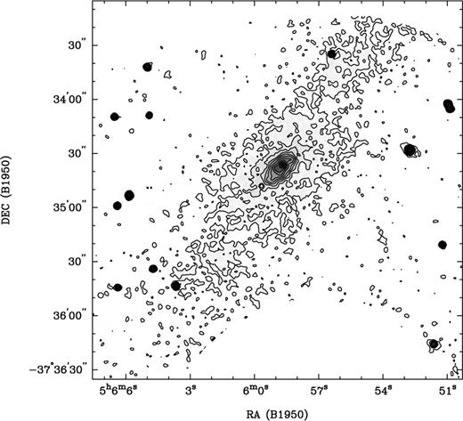
The NGC 1808 optical continuum, after convolution with a 1.8-arcsec (3 pixel wide) Gaussian. The wavelength is centred on ∼6585.4 Å. A circular partially sampled region at the bottom has been masked out owing to its high noise level. Contour levels are 3, 5, 7.1, 10, 14, 20, 28, 40 and 57×10−28 erg cm−2 s−1 Hz−1.

Sample Hα channel maps of NGC 1808. The optical velocity is quoted in each channel, in km s−1. One channel in every 40 km s−1 is shown. Some data to the top and/or bottom of each image were not sampled and are thus blanked. The field of view differs slightly from other figures. Contour levels are 1.5, 3, 6, 12 and 24×10−27 erg cm−2 s−1 Hz−1.
4.3.7 Artefacts
The fact that the available CCD images only sample particular values of z (thus requiring interpolation between known data points), combined with calibration errors and the instrumental response, inevitably produces certain artefacts and errors in phase-corrected images. These can be summarized as follows.
- (i)
The interpolation performed using equation (18) tends to smooth the pixels at any given (x,y) position, along the velocity axis. This could potentially result in output pixels being derived from input pixels out of position by up to one z-plane with respect to equation (13) (∼20 km s−1 for the NGC 1808 data). This should only distort the spectrum significantly if the source cube undersamples the spectrum, i.e. if it has constant-z planes with a spacing comparable to or greater than the spectral resolution of the etalon, so that the observed spectrum changes markedly from one plane to the next.
- (ii)
The response of the etalon produces faint regular ‘rings’ centred on the optic axis, particularly if the ring FWHM (in z) is of a value similar to or smaller than the z-spacing. This looks vaguely similar to the beam artefacts from radio interferometers, except that it does not attenuate with distance and it is centred on only one position in the image. For the NGC 1808 data (Section 5), these rings were at a low level and had no significant effect on observations, and were ignored. However, in other cases they could be reduced by smoothing, for example when a seeing correction was performed.
- (iii)
Poor calibration of the input data, particularly the use of multiple input images that have not been calibrated consistently, or time-variability in the instrumental response, can cause sudden changes in the intensity of output images at certain r-values. This occurs particularly when more than one order n is used to produce the output image, producing a sudden change by one FSR in the z-values of the input data used. Since z is typically scanned sequentially, if the data are poorly calibrated or time-dependent then supposedly equivalent data points in different orders may actually have rather different intensities.
- (iv)
Partially unsampled regions of the (x,y) plane, i.e. where data are not available for all velocities, will affect production of continuum and moment maps for those regions owing to the smaller number of data being averaged together, e.g. by increasing noise. This occurs in circular bands centred on the optic axis as in Fig. 7, or on the ‘outside’ of the image. The approach, which we have used successfully, is to set unsampled phase-corrected data to zero before continuum subtraction. This, however, reduces the fitted continuum intensity in that region.
5 Example: NGC 1808
Using NGC 1808 as an example, the flat-fielded source cube was phase corrected with an optical velocity axis from 620 to 1440 km s−1 in 20 km s−1 increments. Unsampled pixels were set to zero. The line and continuum were separated using the miriad task contsub, using a first-order polynomial continuum fit to the first three (620–660 km s−1) and last six (1340–1440 km s−1) channels. The resulting continuum map is shown in Fig. 7, and some of the Hα channel maps are shown in Fig. 8. Uncertainties in the neon calibration line orders, and hence in A, result in a possible offset of a few km s−1 in the velocity axis, which is not significant at this velocity resolution.
The Hα channel maps were used to form the Hα total intensity and mean velocity (zeroth moment and first moment) maps in Fig. 9. Clearly visible is the nucleus, which shows strong continuum emission, along with a number of knots of Hα, with positions corresponding to the spiral arms or to the bar previously reported (Koribalski 1993; Koribalski et al. 1996). The continuum matches the shape and position of the disk. The flux scale used is the one derived from Hamuy et al. (1982), 2.115×10⁻²⁸ erg cm−2 s−1 Hz−1count−1 (Section 4.1.4).
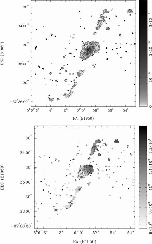
Hα zeroth- and first-moment maps of NGC 1808, obtained using the aips task momnt. Circular regions to the top and bottom were only partially sampled and have been masked to remove noise. There is not thought to be emission in these regions. Top panel: zeroth moment (integrated Hα intensity distribution). Contours are 1, 2, 4, 8, 16, 32, 64 and 128×10−16 erg s−1 cm−2. Bottom panel: first moment (mean Hα velocity field). Contours are 800, 850, 900, 950, 1000, 1050, 1100, 1150 and 1200 km s−1.
6 Conclusion
We have described in detail the observational and data reduction process for astronomical imaging with a Fabry-Perot etalon on an optical telescope. The stages accomplishing instrumental calibration and phase correction are Fabry-Perot specific, and thus not generally supported by reduction software. To remedy this we have written a set of new tasks to perform these stages in the miriad software environment. Using this process and the new software, we have reduced the data from Hα observations of three galaxies, NGC 1808, NGC 2442 and Circinus, made using the TAURUS-2 instrument on the Anglo-Australian Telescope. The NGC 1808 data have been used to illustrate the process and the results obtained. More complete descriptions and analyses of the results for NGC 2442 and Circinus have been published (Houghton 1998, Elmouttie et al. 1998), and those for NGC 1808 will be published in future.
In particular, we have discussed the basic features of Fabry-Perot instruments, the taking of data, the derivation of instrumental parameters, and the process through which the data pass to produce calibrated spectral data cubes of a source, along with moment and continuum maps. The new software has also been described, including the algorithms involved and the limitations imposed. It can be used to produce spectral cubes sampling particular wavelength or velocity ranges. This software is available as a set of additional tasks for the miriad system (used for radio astronomy), but can operate as stand-alone UNIX programs. It is portable and has been used successfully on DEC Alpha computers, Sun workstations and IBM PCs running LINUX.
Acknowledgments
We thank John Whiteoak of the Australia Telescope National Facility, who initiated the observational project described here, and who helped to make the TAURUS-2 observations. We also thank Keith Taylor of the Anglo-Australian Observatory, who assisted with the observations, and who gave us valuable assistance with the data reduction. The fpcal computer program described here uses source code ported from the iraf Fabry-Perot package originally written for CTIO by George Jacoby. This has been used with the permission of Doug Tody, NOAO. We thank the referees for their most valuable comments and suggestions for this paper.
References
For details of CCD imaging at the AAT, see http://www.aao.gov.au/local/www/cgt/ccdimguide/ccd_chap2.html.
Astronomical Image Processing System.
Multichannel Image Reconstruction and Image Analysis and Display: see http://www.atnf/csiro.au/computing/software/miriad/.
Munich Image Data Analysis System.
Image Reduction and Analysis Facility.
For download of the CTIO Fabry-Perot package, see ftp://iraf.noao.edu/iraf/extern; for package information, see http://iraf.noao.edu/cgi-bin/irafhelp?fabry.
Appendix
Appendix A: Step-by-step Guide
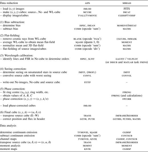
A step-by-step guide to Fabry-Perot data reduction and analysis.
