Weak gravitational lensing in the standard cold dark matter model, using an algorithm for three-dimensional shear

Abstract

1 Introduction

The gravitational lensing of light by the general form of the large-scale structure in the Universe is of considerable importance in cosmology. This ‘weak lensing’ may result in magnification of a distant source from Ricci focusing owing to matter in the beam, and shear leading to distortion of the image cross-section. The strength of these effects depends on the lens and source angular diameter distances and the specific distribution of matter between the observer and source. Consequently the effects are likely to be sensitive to the particular cosmological model. In extreme cases, a source may be strongly lensed if the light passes close to a massive structure such as a galaxy, and reconstruction of the mass profiles for lensing galaxies have been attempted in a number of studies; see, e.g., Falco, Govenstein & Shapiro (1991), Grogan & Narayan (1996), and Keeton & Kochanek (1997). These studies have frequently made use of the ‘thin-screen approximation’ in which the depth of the lens is considered to be small compared with the distances between the observer and the lens and the lens and the source. In the thin-screen approximation the mass distribution of the lens is projected along the line of sight and replaced by a mass sheet with the appropriate surface density profile.

The simplicity of the thin-screen approximation has also lead to its use in weak gravitational lensing studies, where each of the output volumes from cosmological N-body simulations are treated as planar projections of the particle distributions within them. To compute the distributions in magnification and shear for a large number of rays passing through the system of screens, use is made of the multiple lens-plane theory which has been variously described by Blandford & Narayan (1986), Blandford & Kochanek (1987), Kovner (1987), Schneider & Weiss (1988a,b) and summarized by Schneider, Ehlers & Falco (1992). We describe some of these two-dimensional weak lensing methods in Section 1.1.

Couchman, Barber & Thomas (1998) considered some of the shortcomings of these two-dimensional lens-plane methods, and also rigorously investigated the conditions under which two-dimensional methods would give equivalent results to integrating the shear components¹ through the depth of a simulation volume. They showed that, in general, it is necessary to include the effects of matter stretching well beyond a single period in extent, orthogonal to the line of sight, but depending on the particular distribution of matter. It is also necessary to project the matter contained within a full period on to the plane, assuming the distribution of matter in the Universe to be periodic with periodicity equal to the simulation volume side dimension. They also showed that errors can occur in two-dimensional approaches because of the single angular diameter distance to each plane, rather than specific angular diameter distances to every location in the simulation volume.

These considerations motivated Couchman et al. (1998) to develop an algorithm to evaluate the shear components at a large number of locations within the volume of cubic particle simulation time-slices. In this paper we have applied the algorithm to the standard cold dark matter (sCDM) cosmological N-body simulations available from the Hydra consortium,² which we describe in Section 2.2. By combining the outputs from the algorithm from sets of linked time-slices going back to a redshift of 4, we are able to evaluate the overall shear, convergence, magnifications and source ellipticities (and distributions for these quantities). We first describe other work which has generated results from studies of weak lensing in the sCDM cosmology.

1.1 Other work

There are numerous methods for studying weak gravitational lensing. In ‘ray-tracing,’ (see, for example, Schneider & Weiss 1988b, Jaroszyński et al. 1990, Wambsganss, Cen & Ostriker 1998, Marri & Ferrara 1998, Jain, Seljak & White 1998, and Jain, Seljak & White 1999) the paths of individual light rays are traced backwards from the observer as they are deflected at each of the projected time-slice planes. The mapping of these rays in the source plane then immediately gives information about the individual amplifications which apply. In the ‘ray-bundle’ method, (see, for example, Fluke, Webster & Mortlock 1999, and Premadi, Martel & Matzner 1998a,b,c), bundles of rays representing a circular image are considered together, so that the area and shape of the bundle at the source plane, (after deflections at the intermediate time-slice planes), gives the required information on the ellipticity and magnification. We shall describe briefly five works which have produced weak lensing results in the sCDM cosmology.

Jaroszyński et al. (1990) use the ray-tracing method with two-dimensional planar projections of the time-slices, and by making use of the assumed periodicity in the particle distribution, they translate the planes for each ray, so that it becomes centralized in the plane. This ensures that there is no bias acting on the ray when the shear is computed. Each plane is divided into a regular array of pixels, and the column density in each pixel is evaluated. Instead of calculating the effect of every particle on the rays, the pixel column densities in the single period plane are used. They calculate the two two-dimensional components of the shear (see Section 5 for the definition of shear) as ratios of the mean convergence of the beam, which they obtain from the mean column density. However, they have not employed the net zero mean density requirement in the planes, (described in detail by Couchman et al. 1998), which ensures that deflections and shear can only occur when there are departures from homogeneity. Also, the matter in the pixel through which the ray is located is excluded. Their probability distributions for the convergence, owing to sources at redshifts of 1, 3 and 5, are therefore not centralized around zero, and exhibit only limited broadening for sources at higher redshift. They also display the probability distributions for the shear and the corresponding distributions for source ellipticity. (The procedures used by Jaroszyński 1991, and Jaroszyński 1992, are improved by the introduction of softening to each particle to represent galaxies of different masses and radii.)

Wambsganss et al. (1998) also use the ray-tracing method with two-dimensional planar projections of the simulation boxes, which have been randomly oriented. Rays are shot through the central region of 8 h⁻¹ Mpc×8 h⁻¹ Mpc only (where h is the Hubble parameter expressed in units of 100 km s⁻¹ Mpc⁻¹) and the deflections are computed by including all the matter in each plane, allocated to pixels 10 h⁻¹ kpc×10 h⁻¹ kpc, covering one period in extent only. The planes have comoving dimensions of 80 h⁻¹ Mpc×80 h⁻¹ Mpc. By using the multiple lens-plane theory, they show both the differential magnification probability distribution, and the integrated one for 100 different source positions at redshift z_s=3.0. One advantage of this type of ray-tracing procedure is its ability to indicate the possibility of multiple imaging, where different rays in the image plane can be traced back to the same pixel in the source plane.

Premadi et al. (1998a) have improved the resolution of their N-body simulations by using a Monte Carlo method to locate individual galaxies inside the computational volume, and ensuring that they match the two-point correlation function for galaxies. They also assign morphological types to the galaxies according to the individual environment, and apply a particular surface density profile for each. To avoid large-scale structure correlations between the simulation boxes, five different sets of initial conditions are used for the simulations, so that the individual plane projections can be selected at random from any set. By solving the two-dimensional Poisson equation on a grid, and inverting the equation using a Fast Fourier Transform (FFT) method, they obtain the first and second derivatives of the gravitational potential on each plane. They also correctly ensure that the mean surface density in each lens-plane vanishes, so that a good interpretation of the effects of the background matter is made. Their method uses beams of light, each comprising 65 rays. They show the average shear for a source at z_s=5 contributed by each of the lens-planes individually, and find that the largest contributions come from those planes at intermediate redshift, of order z=1–2. Similarly, they find that the lens-planes which contribute most to the average magnifications are also located at intermediate redshifts. The multiple lens-plane theory then enables the distributions of cumulative magnifications to be obtained, which are shown to be broad and similar in shape for the sCDM and cosmological constant models, although the latter model shows a shift to larger magnification values.

Marri & Ferrara (1998) use a total of 50 lens-planes evenly spaced in redshift up to z=10. Their mass distributions have been determined by the Press—Schechter formalism (which they outline), which is a complementary approach to N-body numerical simulations. From this method they derive the normalized fraction of collapsed objects per unit mass for each redshift. They acknowledge that the Press-Schechter formalism is unable to describe fully the complexity of extended structures, the density profile of the collapsed objects (the lenses), or their spatial distribution at each redshift. They therefore make the assumption that the lenses are spatially uncorrelated and randomly distributed on the planes, and furthermore behave as point-like masses with no softening. In their ray-tracing approach they follow 1.85×10⁷ uniformly distributed rays. The final impact parameters of the rays are collected in an orthogonal grid of 300² pixels in the source plane. Because of the use of point masses, their method produces very high magnification values, greater than 30 for the sCDM cosmology. They have also chosen to use a smoothness parameter in the redshift-angular diameter distance relation (which we describe in Section 3) which depicts an entirely clumpy universe.

Jain et al. (1998, 1999) have compared weak lensing results for four different cosmologies using N-body simulations with 256³ particles generated using a parallel adaptive AP³M code. Their ray-tracing algorithm first projects the dark matter distribution from each simulation box onto equally spaced lens-planes between the source and the observer. Usually each plane is the same angular size as the face of the simulation box would be at the source redshift, and the orientation of each is random. Secondly, the shear matrix is computed on a grid within each plane using a Fourier Transform of the projected density and periodic boundary conditions. Perturbations on the (more than 10⁶) photon trajectories are computed and the shear matrix interpolated to the photon positions. The resulting Jacobian matrix (see equation 7) is then computed in accordance with the multiple lens-plane theory. From this data they are able to determine the power spectrum in both the shear and the convergence, and find them to be almost entirely in the non-linear regimes and in good agreement with non-linear analytical predictions. The non-linear effects are strongest in the sCDM cosmology. They also show the non-Gaussian features in the one-point distribution function for the convergence and its sensitivity to the density parameter in the different cosmologies.

1.2 Outline of paper

In Section 2.1 we summarize the main features of the algorithm for shear in three dimensions, which is detailed in Couchman et al. (1998). In Section 2.2 we describe the sCDM N-body simulations and how we combine the different output time-slices from the simulations to enable the integrated shear along lines of sight to be evaluated.

Because we evaluate the shear at locations throughout the volume of the simulation boxes, and because of some sensitivity (see Couchman et al. 1998) of the results to the smoothness, or clumpiness, of the matter distribution in the universe, we consider, in Section 3, our choice of the appropriate angular diameter distances. We consider the effects of shear on the angular diameter distance, and the sensitivity of our results to the smoothness parameter, . Measurements of the particle clustering within our simulations, which determines the variable softening parameter for use in the shear algorithm, also enable a good definition for the smoothness parameter to be made, and this is discussed.

In Section 4, we describe the formation of structure within the universe as it evolves, in terms of the magnitudes of the shear components computed for each time-slice. We see how the rms values of the components vary with redshift, and also how the set of highest values behave. We also identify, in terms of the lens redshifts, where the significant contributions arise. Our conclusions are compared with the results of other authors.

In Section 5, we describe in outline the multiple lens-plane theory, with particular reference to our application of it. In Section 6, we discuss our results for the shear, convergence, magnifications, source ellipticities, distributions of these values, and relationships amongst them.

Our findings are summarized in Section 7, where we compare and contrast the results with those of other authors who have used two-dimensional approaches for the sCDM cosmology, and which, in general, are different from our findings. We also point to considerable differences between our magnification distributions obtained for sources at redshifts of 1 and 0.5 and those used by Wambsganss et al. (1997) who attempted to assess the impact on the perceived value of the deceleration parameter obtained from high-redshift Type Ia supernovae data. We mention, in addition, some other important applications of our results.

2 The algorithm for three-dimensional shear, and the cosmological simulations

2.1 Description of the three-dimensional algorithm

The algorithm we are using to compute the elements of the matrix of second derivatives of the gravitational potential has been described fully in Couchman et al. (1998). The algorithm is based on the standard P³M method (as described in Hockney & Eastwood 1988), and uses a FFT convolution method. It computes all of the six independent shear component values at each of a large number of selected evaluation positions within a three-dimensional N-body particle simulation box. The P³M algorithm has a computational cost of order N log ₂N, where N is the number of particles in the simulation volume, rather than O(N²) for simplistic calculations based on the forces on N particles from each of their neighbours. For ensembles of particles, used in typical N-body simulations, the rms errors in the computed shear component values are typically ∼0.3 per cent.

In addition to the speed and accuracy of the shear algorithm, it has the following features.

First, the algorithm uses variable softening designed to distribute the mass of each particle within a radial profile which depends on its specific environment. In this way we are able to set individual mass profiles for the particles which enables a physical depiction of the large-scale structure to be made. Our choice for the appropriate variable softening has been described fully in Couchman et al (1998), who also describe the sensitivity of the magnification distributions to the choice of the minimum softening value. The minimum level set is 0.001 in box units, which we have allowed to remain at a fixed physical dimension throughout the redshift range of the simulations. Thus, we have set the value to be 0.001 for the z=0 simulation box, rising to 0.0046 in the earliest simulation box at z=3.6. At a redshift of 0.5 the minimum softening value used is 0.0015, which is comparable to the maximum value of the Einstein radius, 0.0014 in box units, for a large cluster of 1000 particles and a source at our maximum redshift of 3.9. At the same time, this scale is approximately of galactic dimensions, giving a realistic interpretation to the choice.

Secondly, the shear algorithm works within three-dimensional simulation volumes, rather than on planar projections of the particle distributions, so that angular diameter distances to every evaluation position can be applied. It has been shown (Couchman et al. 1998) that in specific circumstances, the results of two-dimensional planar approaches are equivalent to three-dimensional values integrated throughout the depth of a simulation box, provided the angular diameter distance is assumed constant throughout the depth. However, by ignoring the variation in the angular diameter distances throughout the box, errors up to a maximum of 9 per cent can be reached at a redshift of z=0.5 for sCDM simulation cubes of comoving side 100 h⁻¹ Mpc. (Errors can be larger than this at high and low redshift, but the angular diameter distance multiplying factor for the shear values is greatest here for sources we have chosen at a redshift of 4.)

Thirdly, the shear algorithm automatically includes the contributions of the periodic images of the fundamental volume, essentially creating a realization extending to infinity. Couchman et al. (1998) showed that it is necessary to include the effects of matter well beyond the fundamental volume in general (but depending on the particular particle distribution), to achieve accurate values for the shear. Methods which make use of only the matter within the fundamental volume may suffer from inadequate convergence to the limiting values.

Fourthly, the method uses the ‘peculiar’ gravitational potential, φ, through the subtraction of a term depending upon the mean density. Such an approach is equivalent to requiring that the net total mass in the system be set to zero, and ensures that we deal only with light ray deflections arising from departures from homogeneity; in a pure Robertson—Walker metric we would want no deflections.

2.2 The sCDM large-scale structure simulations

We have chosen, in this paper, to apply the shear algorithm to the sCDM cosmological N-body simulations available from the Hydra consortium, and produced using the ‘Hydra’N-body hydrodynamics code, as described by Couchman, Thomas & Pearce (1995). Each time-slice from this simulation contains 128³ dark matter particles, each of 1.2×10¹¹h⁻¹ solar masses, with a CDM spectrum in an Einstein—de Sitter universe, and has comoving box sides of 100 h⁻¹ Mpc. The output times for each time-slice have been chosen so that consecutive time-slices abut, enabling a continuous representation of the evolution of large-scale structure in the Universe. However, to avoid unrealistic correlations of the structure through consecutive boxes, we arbitrarily rotate, reflect and translate the particle coordinates in each before the boxes are linked together. We have chosen to analyse all the simulation boxes back to a redshift of 3.9, a distance which is covered by a continuous set of 33 boxes (assuming the source in this case at z_s=3.9 to be located at the far face of the 33rd box, which has a nominal redshift of 3.6). The simulations used have a power spectrum shape parameter of 0.5, and the normalization, σ₈, has been taken as 0.64 to reproduce the number density of clusters, according to Vianna & Liddle (1996).

We establish a regular array of 100×100 lines of sight through each simulation box, and compute the six independent shear components at 1000 evenly spaced evaluation positions along each. The 1000 evaluation positions on each line of sight is well matched to the minimum variable softening, giving adequate sampling in the line of sight direction; we have tested our method using up to a total of 4×10⁶ lines of sight, and have found that whilst this smooths the distribution plots of Section 6 at the high magnification end and gives rise to higher maximum values of the magnification, the statistical widths of the plots are virtually unchanged. Since we are dealing with weak lensing effects and are interested only in the statistical distribution of values, these lines of sight adequately represent the trajectories of light rays through each simulation box. It is sufficient also to connect each ‘ray’ with the corresponding line of sight through subsequent boxes in order to obtain the required statistics of weak lensing. This is justified because of the random re-orientation of each box performed before the shear algorithm is applied.

3 Angular diameter distances

One of the advantages of being able to evaluate the shear components at a large number of locations within the volume of each time-slice is that we are able to apply the appropriate angular diameter distance factors to each as part of the procedure to determine the magnifications and ellipticities. The Jacobian matrix at each evaluation position,

(1)

is used to determine the magnification at that point, and contains the two-dimensional effective lensing potentials which are related to the computed three-dimensional shear, ∂²φ/∂x_i∂x_j, through

(2)

where D_d, D_ds, and D_s are the angular diameter distances from the observer to the lens, the lens to the source, and the observer to the source, respectively, and c is the velocity of light. The integration is along the line of sight. The angular diameter distances depend very much on the distribution of matter, so that it is necessary to have available appropriate values for the particular distribution being investigated.

Dyer & Roeder (1972, 1973) made assumptions about the type of matter distribution to obtain a second-order differential equation for the angular diameter distance in terms of the density parameter, Ω, for the universe, and the redshift of the source:

(3)

is the smoothness parameter, which is taken to be the fraction of mass in the universe which is smoothly distributed, and σ is the optical scalar for the shear, introduced by matter surrounding the beam. They considered the convenient scenario in which the light beams travel through the homogeneous low density, or empty regions, passing far away from the clumps, so that the shear becomes negligible. However, we must consider whether the shear in our particle simulation time-slices is able to significantly affect our chosen values for the angular diameter distances.

Schneider & Weiss (1988a) showed that, in general, the effects of shear must be taken into account. For rays weakly affected by shear and with low amplifications, the linear terms in the shear almost cancel, but higher order terms become more important. However, the probability for rays being affected by shear is dramatically lower in model universes with compared with universes with . (We shall show shortly that the values of in our sCDM simulations are always at least 0.83, so that even at z=0 the matter distribution may be considered smooth according to the usual definition of .) In summary, we might expect the number of rays affected by shear to be low in smooth matter distributions, and then the effect to be only of second order.

Watanabe & Tomita (1990) concluded that, on average, the effect of shear on the distance-redshift relation is small, providing the scale of the inhomogeneities is greater than or equal to galactic scales. This is in agreement with Futamase & Sasaki (1989) who showed that, in most cases, the shear does not contribute to the amplification.

Our own work is conducted using a cosmological simulation in which the distribution of matter is very smooth. Furthermore, our minimum softening scale is of the order of galactic dimensions, so that we feel justified in accepting that the shear plays only a second-order role in the distance—redshift relation in our sCDM data-set. (We are able to quantify the effects of shear from our results in Section 6, and find that they are negligible.) With σ∼0, therefore, equation (3) immediately reduces to the well-known Dyer—Roeder equation which has the following generalized solution for the angular diameter distance between redshifts of z₁ and z₂ for Ω=1:

(4)

β is expressed in terms of arbitrary :

(5)

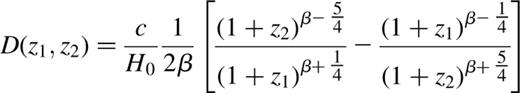
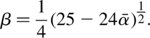
We can write the left hand side of equation (4), equivalently, as in which r(z₁,z₂) is the dimensionless angular diameter distance. We show in Fig. 1 the value of the dimensionless multiplying factor, R≡r_dr_dsr_s, as it applies to different time-slices at different redshifts, assuming sources at z_s=3.9, 3.0, 1.9, 1.0 and 0.5. (These values correspond to the redshifts of our time-slices, and have been chosen to be close to z=4, 3, 2, 1 and 0.5.) We have assumed zero shear, a completely smooth distribution of matter, and Ω=1. We see that the peak in this factor occurs near z=0.5 for a source at redshift 4.

Figure 1.

The dimensionless multiplying factor, Rr_dr_{d s}r_s, assuming sources at different redshifts. The uppermost curve for a source at z_s=4, peaks at z=0.52; the next curve is for z_s=3 and peaks at z=0.48; the next curve is for z_s=2 and peaks at z=0.40; the next curve is for z_s=1 and peaks at z=0.32; the lowest curve is for z_s=0.5 and peaks at z=0.20.

Open in new tabDownload slide

From the output of our algorithm we are able to obtain an estimate of the clumpiness or smoothness in each time-slice. In the earliest time-slice at z=3.6, (next to z=3.9), there is a mass fraction of 0.026 in clumps, giving and at z=0 the fraction is 0.17, giving . Whilst we have not accurately tried to assess the mean value for extending to different source redshifts, it is clear that the value throughout is close to 1, and almost equivalent to the ‘filled beam’ approximation. This result concurs with Tomita (1998) who finds to be close to 1 in all cases. We show in Fig. 2 how similar the multiplying factor is for the values and 1.0, and how these compare with a value of for an entirely clumpy universe. The maximum discrepancy between and is 5.2 per cent for a source at z_s=4, 2.4 per cent for z_s=2, and for sources nearer than z_s=1 the maximum discrepancy is well below 1 per cent. We have compared the sCDM cosmology with alternative simulations using a power spectrum shape parameter of 0.25 as determined experimentally on cluster scales (see Peacock & Dodds 1994), and find that then the smoothness parameter varies only between 0.88 and 0.99, i.e., a much narrower range and closer to unity. This confirms that the sCDM cosmology (with shape parameter 0.5) gives rise to more clumpiness at late times, allowing higher values of magnification and shear to occur.

Figure 2.

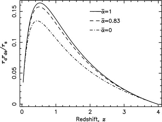
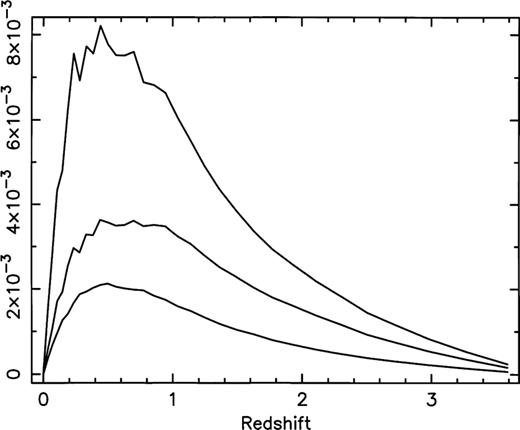
The multiplying factor, r_dr_{d s}r_s, for a source at redshift 4, with smoothness parameters of 1 (uppermost curve), 0.83 (middle curve), and 0 (lowest curve).

Open in new tabDownload slide

4 The formation of structure

In this section we consider the values of the two-dimensional effective lensing potentials (calculated using equation 2) in each time-slice. Without at first applying the angular diameter distance multiplying factors, we can, in a simplistic way, obtain values which characterize each time-slice, independent of its redshift, to give information about the development of structure.

The shear algorithm generates the six independent three-dimensional shear component values (expressed in box units), and we have chosen to compute them at 1000 evaluation positions along 100×100 lines of sight in each simulation time-slice. It is then possible to evaluate the two-dimensional effective lensing potentials independently, using equation 2, at each of, say, 50 locations along every line of sight by integrating the component values and converting to physical units. The integration of the values in this way and the conversion to physical units requires the computed values to be multiplied by the factor B(1+z)²r_dr_{d s}r_s, where B=(cH₀)(2/c²)GM_part×(comoving box depth)⁻². (G is the universal gravitational constant and M_part is the particle mass.) For the simulation boxes we have used, which have comoving dimensions of 100 h⁻¹ Mpc, B=3.733×10⁻⁹. The (1+z)² factor occurs to convert the comoving code units to physical units.

By integrating the values and applying only the factor B(1+z)² (without the angular diameter distance factor), we obtain the characteristic values for each time-slice. The middle curve of Fig. 3 shows the rms values for the sum of the diagonal terms in equation (2) calculated in this way for each time-slice. These values are closely associated with the surface density, which in turn determines the magnifications produced in the time-slice. We notice that the values for these combined components very slowly decreases towards z=0. This same trend is apparent with the other components individually. It has the interesting interpretation that, even though structure is forming (to produce greater magnification locally), the real expansion of the universe (causing the mean particle separation to increase) just outweighs this in terms of the magnitudes of the component values. Nevertheless, the formation of structure can be seen; the top curve in Fig. 3 shows the result of taking the mean of just the set of highest values in each time-slice, again multiplied only by the factor B(1+z)². This shows an initial fall as the universe expands and before structure has begun to form, and then at later times an increase in the mean values, indicative of the existence of dense (bound) structures. The lowest curve in Fig. 3 shows the set of highest values for one of the off-diagonal components, including the multiplication by B(1+z)², and this shows a similar trend.

Figure 3.

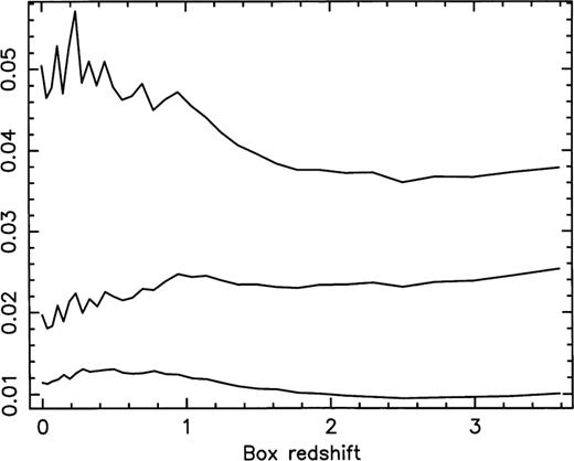
Curves characterizing the time-slices, established without the inclusion of the angular diameter distance multiplying factors. Middle curve: the rms value in each time-slice of the sum of the diagonal elements of the Jacobian matrix. Top curve: the mean of the highest values of the summed diagonal elements. Lowest curve: the mean of the highest values for one of the off-diagonal elements.

Open in new tabDownload slide

However, when the computed values are multiplied by the full conversion factors, including the angular diameter distance factors, r_dr_{d s}r_s(≡R), we see in Fig. 4 that the peaks are extremely broad, indicating that significant contributions to the magnifications and ellipticities can arise in time-slices covering a wide range of redshifts, and not just near z=0.5 where R has its peak (for sources at z_s=4).

Figure 4.

Components in each time-slice converted to absolute values, including the angular diameter distance factors, for sources at z_s=4. Middle curve: the rms value in each time-slice of the sum of the diagonal elements of the Jacobian matrix. Top curve: the mean of the highest values of the summed diagonal elements. Lowest curve: the mean of the highest values for one of the off-diagonal elements.

Open in new tabDownload slide

Premadi et al. (1998a) have performed similar work. For the shear and magnification they find that the individual contribution owing to each of their lens-planes is greatest at intermediate redshifts, of order z=1–2, for sources located at z_s=5. Premadi et al. (1998b,c) also report their results for the shear for sources at z_s=3, and again find very broad peaks covering a wide range of (intermediate) lens-plane redshifts.

5 Multiple lens-plane theory

As described in Section 2.2, we establish 1000 evaluation positions along each of the 100×100 lines of sight through each simulation time-slice, and the shear algorithm computes the six independent second derivatives of the gravitational potential at each position. By integration of the computed values using equation (2), we establish the matrices of two-dimensional effective lensing potentials,

(6)

at each of 50 positions along every line of sight in each simulation box. (We may take because we are dealing with a weak shear field which is smoothed by the variable particle softening, ensuring that the gravitational potential and its derivatives are well-behaved continuous functions.) The Jacobian matrix, A, is then evaluated at successive positions along each line of sight as it develops in accordance with the multiple lens-plane theory, which is summarized by Schneider et al. (1992). The final Jacobian matrix after N deflections is

(7)

where I is the unit matrix, and the intermediate Jacobian matrices are

(8)

where

(9)

in which D_j, D_is and D_ij are the angular diameter distances to the jth lens, that between the ith lens and the source, and that between the ith and jth lenses, respectively.

The magnification, μ, at any position, is given in terms of the Jacobian at that point:

(10)

so that we can assess the magnification as it develops along a line of sight, finally computing the emergent magnification after passage through an entire box or set of boxes. The convergence, κ, is defined by

(11)

from the diagonal elements of the Jacobian matrix, and causes isotropic focussing of light rays, and so isotropic magnification of the source. Thus, with convergence acting alone, the image would be the same shape as, but a different size from, the source.

The shear, γ, in each line of sight, is given by

(12)

Shear introduces anisotropy, causing the image to be a different shape, in general, from the source.

From equation (10), and these definitions,

(13)

so that with weak lensing the magnification reduces to

(14)

In the presence of convergence and shear, a circular source becomes elliptical in shape, and the ellipticity, ɛ, defined in terms of the ratio of the minor and major axes, becomes

(15)

which reduces to

(16)

in weak lensing.

The multiple lens-plane procedure allows values and distributions of the magnification, ellipticity, convergence and shear to be obtained at z=0 for light rays traversing the set of linked simulation boxes starting from the chosen source redshift. The ability to apply the appropriate angular diameter distances at every evaluation position avoids the introduction of errors associated with planar methods, and also allows the possibility of choosing source positions within a simulation box if necessary. This may be useful when considering the effects of large-scale structure on real observed sources at specific redshifts, or if the algorithm is to be applied to large simulation volumes.

6 Results

We first examine the importance of the smoothness parameter, , in the distance-redshift relation, to the magnification distribution, by computing the magnifications owing to a single (assumed isolated) simulation box at z=0.5 for a source at z_s=4. (At this box redshift the contribution to the magnifications is expected to be near the maximum.) The magnification distributions arising for and (deduced from our simulations, as explained in Section 3) are virtually indistinguishable, with differences occuring only at the high magnification (low probability) ends of the distributions. The distributions covering the full range of redshift, using all the simulation boxes, show a small sensitivity to the smoothness parameter. We have chosen therefore to present our results based on a smoothness parameter of throughout.

We have chosen to assume source redshifts, z_s, close to 4, 3, 2, 1 and 0.5, and shall refer to the sources in these terms. The actual redshift values are 3.9, 3.0, 1.9, 1.0 and 0.5 respectively, corresponding to nominal time-slice redshifts in our sCDM simulation. For each source redshift we have evaluated the final emergent Jacobian matrix at z=0 for all 10000 lines of sight, by linking all the simulation boxes between the source redshift and z=0, as described in Section 5, and, by manipulation of the data according to the multiple lens-plane equations, we have been able to produce all the required values for the magnifications, ellipticities, shear and convergence.

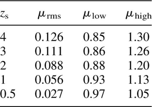
Figs 5 and 6 show the distributions of the magnifications, μ, for the five source redshifts, and for all source redshifts there is a significant range. The rms fluctuations for the magnifications about the mean value of 〈μ〉=1 are displayed in column 2 of Table 1 for each source redshift. However, since the magnification distributions are asymmetrical, we have calculated the values, μ_low and μ_high, above and below which 97.5 per cent of all lines of sight fall. These are displayed in columns 3 and 4 of Table 1. The values contrast with the values obtained from the alternative cosmology with a power spectrum shape parameter of 0.25 which are displayed in Table 2. In general we find that the distributions for the magnifications, convergence, shear and ellipticities are all broader in the sCDM cosmology (with shape parameter 0.5). This is as a result of the more clumpy character of the sCDM cosmology.

Figure 5.

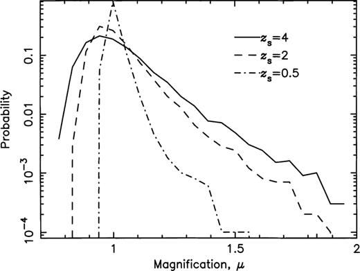
Probability distributions for the magnification, for z_s=4, 2 and 0.5.

Open in new tabDownload slide

Figure 6.

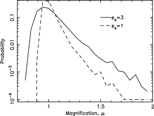
Probability distributions for the magnification, for z_s=3, and 1.

Open in new tabDownload slide

Table 1.

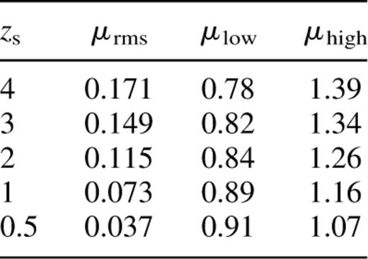
SCDM cosmology. Column 2 shows the rms fluctuations for the magnifications, μ_rms, about the mean value of 〈μ〉=1 for the various source redshifts, z_s; column 3 shows the magnification value μ_low for each redshift above which 97.5 per cent of all lines of sight fall; column 4 shows the magnification values μ_high for each redshift below which 97.5 per cent of all lines of sight fall.

Open in new tabDownload slide

Table 2.

As for Table 1, but alternative cosmology with power spectrum shape parameter 0.25.

Open in new tabDownload slide

The accumulating number of lines of sight having magnifications greater than the abscissa value is shown in Fig. 7 for the five different source redshifts, and clearly shows the distinctions at the high magnification end.

Figure 7.

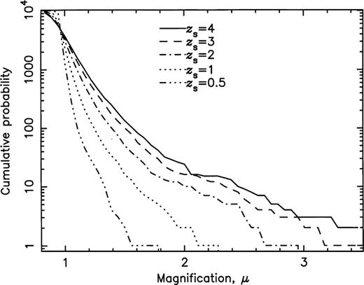
The accumulating number of lines of sight with magnifications greater than the abscissa value, for z_s=4, 3, 2, 1 and 0.5.

Open in new tabDownload slide

In Fig. 8 we show the magnification, μ, plotted against the convergence, κ, for z_s=4, and see that the magnification is clearly not linear in κ as expected for small magnitudes of κ. This is true for all our source redshifts. The non-linearity arises because of the presence of the higher order terms in the expression for μ given by equation (14), and we show for comparison the curve of μ=1+2κ+3κ².

Figure 8

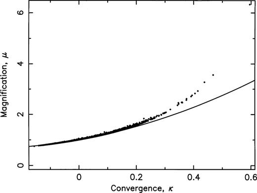
μ versus κ for z_s=4 (dots). The continuous line, shown for comparison, represents μ=1+2κ+3κ².

Open in new tabDownload slide

We would generally expect the shear, γ, to fluctuate strongly for light rays passing through regions of high density (high convergence), and we indeed find considerable scatter in the shear when plotted against the convergence. Fig. 9, however, shows the result of binning the convergence values and calculating the average shear in each bin, for sources at z_s=4. We see that throughout most of the range in κ the average shear increases very slowly, and closely linearly. (At the high κ end there are too few data points to establish accurate average values for γ.) This result suggests that there may be a contribution to the magnification from the shear, and we discuss this later in this section.

Figure 9.

Shear versus convergence for sources at z_s=4 (dots), and the average shear (full line) in each of the κ bins, which shows a slow and nearly linear increase with increasing convergence.

Open in new tabDownload slide

Fig. 10 shows the distributions in the convergence, κ, primarily responsible for the magnifications. The rms values for the convergence are 0.064 (for z_s=4), 0.058 (for z_s=3), 0.047 (for z_s=2), 0.031 (for z_s=1) and 0.016 (for z_s=0.5). These values are entirely consistent with the rms fluctuations for the magnification about the mean (stated above), being slightly below half the rms magnification values (see equation 14).

Figure 10.

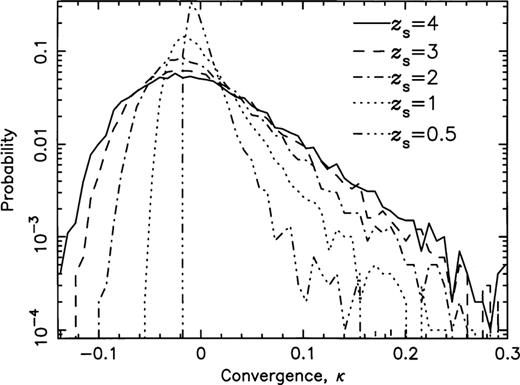
The probability distributions for the convergence, κ, for the five different source redshifts.

Open in new tabDownload slide

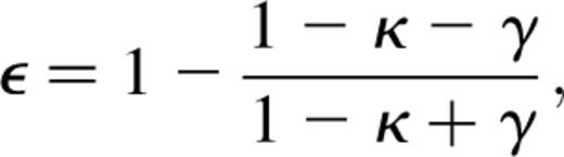
The distributions in the shear, γ, (defined according to equation 12) for the five source redshifts, are broadest, as expected, for the highest source redshifts, and, for z_s=4, 97.5 per cent of all lines of sight have shear values below 0.126. The ellipticity, ɛ, in the image of a source is primarily produced by the shear, and we show in Fig. 11 the distributions in ɛ for the five source redshifts. The peaks in the ellipticity distributions occur at ɛ=0.075 for z_s=4, 0.075 for z_s=3, 0.057 for z_s=2, 0.034 for z_s=1 and 0.016 for z_s=0.5. Fig. 12 displays the accumulating number of lines of sight with ɛ greater than the abscissa value. For z_s=4, we find that 97.5 per cent of all lines of sight have ellipticities up to 0.23. In Fig. 13 we see that the ellipticity is very closely linear in terms of γ throughout most of the range in γ. The scatter arises because of the factor containing the convergence, κ, in equation (16).

Figure 11.

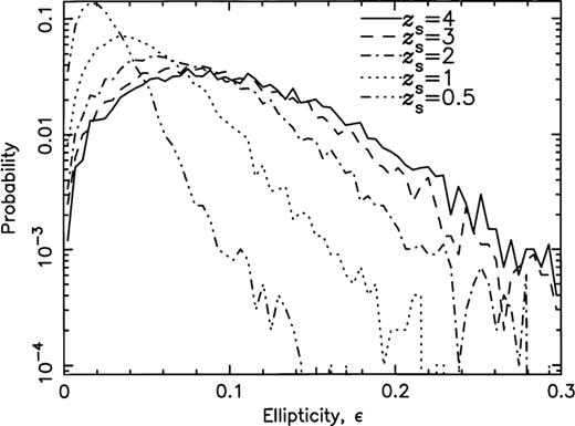
The probability distributions for the ellipticity, ɛ, for the five different source redshifts.

Open in new tabDownload slide

Figure 12.

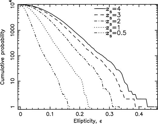
The accumulating number of lines of sight with ɛ greater than the abscissa value, for the five source redshifts.

Open in new tabDownload slide

Figure 13.

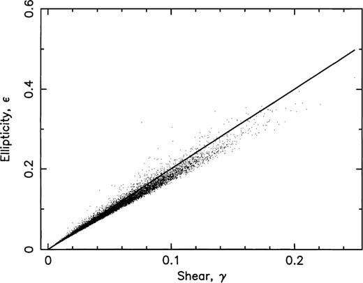
Source ellipticity versus shear for z_s=4 (dots). The straight line, shown for comparison, represents ɛ=2γ.

Open in new tabDownload slide

Finally, we attempted to see if there was a contribution to the magnification from the shear as implied by the distance—redshift relation (equation 3). We found considerable scatter, as expected, in the plots of magnification versus shear, but we found in Fig. 9 a tenuous connection between the shear and the convergence, indicating that there may be a similar connection between the magnification and the shear. We see from equation (14) that the effect of shear is only of second order (as established by Schneider & Weiss 1988a). By binning the shear values and calculating the average magnification in each bin, we are able to show (Fig. 14) that there may be a slow increase in 〈μ〉 with increasing shear. Fig. 14 is for sources at z_s=4. Although there are insufficient data points at the high shear end, it still seems likely that the effects of shear on the mean magnification may be at least 10 per cent for shear values greater than about 0.12. However, interestingly, only 3.2 per cent of the data points in our simulation produced shear in excess of 0.12. According to equation (3), the shear has an effect in the distance-redshift relation equivalent to increasing the effective smoothness parameter, . However, by substituting the mean shear value determined for sources at z_s=0.5 the effect on is found to be completely negligible. Furthermore, the importance of the effect reduces with redshift, so that our conclusion in Section 3, to ignore the effects of shear in the distance—redshift relation, can now be justified.

Figure 14.

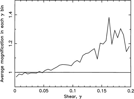
The average magnification in each shear bin, for sources at z_s=4. The overall mean magnification at 〈μ〉=1 is shown for comparison.

Open in new tabDownload slide

7 Discussion of results

In our own work we have had to consider what appropriate angular diameter distance values should be applied to our data. Our decision to ignore the effects of shear in the distance—redshift relation (equation 3) in general is justified because we found that significant effects may occur only in ∼3.2 per cent of the lines of sight, and the impact on the effective value of the smoothness parameter, , by substituting the mean values of the shear, is completely negligible at all redshifts.

We also needed to include a suitable value for the smoothness parameter, , and we found that it varied between approximately 0.97, in the z=3.6 time-slice, and 0.83, at z=0. We checked the significance for the angular diameter distance multiplying factor with these extreme values, and we also investigated the effects of on the magnification distributions. As a result of this work we chose to proceed with our analysis for the sCDM cosmology on the basis of .

In Section 4 we studied the ‘intrinsic’ computed shear values before the application of the angular diameter distance multiplying factors. We found that the universal expansion just outweighs the formation of structure when viewed in terms of the shearing on light. The formation of structure could be seen by considering only the sets of highest values in each time-slice, and then the mean values of these initially fall, before increasing slowly at the onset of structure formation. When the appropriate angular diameter distance multiplying factors were applied to the computed values, we then found the further interesting result that there can be considerable contributions to the shear and magnification arising from time-slices covering a very broad range of redshifts. It will be very interesting in the future to compare these results with those from different cosmologies.

In Section 6 we showed results based on sources at five different redshifts, namely z_s=4, 3, 2, 1 and 0.5. We showed distributions in the magnification (and details of the high magnification end of these distributions), the convergence and the ellipticity (which closely resembles the distribution in the shear), and also the relationships amongst these various quantities. Fig. 8 shows the strong departure from the linear regime for the magnification as a function of the convergence, whilst Fig. 13 shows a closely linear relationship between the ellipticity and the shear. Fig. 9 suggests a slow increase in shear with increasing convergence, broadly as expected. For sources at z_s=4, 97.5 per cent of all lines of sight have magnification values up to 1.39. (The maximum magnifications depend on the choice of the minimum softening in the code, although the overall distributions are very insensitive to the softening.) In particular, we found rms fluctuations in the magnification (about the mean) as much as 0.171 for sources at z_s=4. Even for sources at z_s=0.5 there is a measurable range of magnifications up to 1.07 for 97.5 per cent of the lines of sight.

Of particular importance is how the results of Section 6 may vary with the cosmology and how our results compare with those of other workers. We shall report on the results from other cosmologies in a future publication, and shall discuss here the comparisons of our present results with those other authors whose methods were summarized in the Introduction.

Because of the way in which Jaroszyński et al. (1990) determine the magnifications, their distributions do not have mean magnifications of 1. In addition, their dispersions in the convergence for sources at z_s=1 and z_s=3 can be seen to be considerably lower than our values and they appear to show very little evolution with redshift. Unfortunately their method does not assume a net zero mean density for the projected mass distribution, or make use of the periodic images of each lens-plane. The smoothing of the mass distribution is essentially in terms of the pixellation in each lens-plane.

Wambsganss et al. (1998)find magnifications up to 100 and correspondingly highly dispersed distributions, very much larger than ours for z_s=3. (Their magnification distributions show separately the results for multiply-imaged sources and singly-imaged sources.) The very wide distributions they find have also enabled them to support a μ⁻² power-law tail in the distribution which is predicted by Schneider et al. (1992)in the case of magnification by point sources when μ≫1. The high magnification tail in the distributions almost certainly derives from the low value of the (fixed) softening scale resulting from the ‘smearing’ of the mass distribution in the 10 h⁻¹ kpc×10 h⁻¹ kpc pixels. One advantage of their method is the ability to observe strong lensing events, but a disadvantage may be the fixed softening which makes the large-scale structure (responsible for weak lensing) difficult to represent.

The magnification distributions of Premadi et al. (1998a) appear incomplete, but the range in magnifications appears to be rather similar to ours for sources at z_s=3. This is reassuring because, although their method relies on two-dimensional projections of the simulation boxes, they include many of the essential features to which we have drawn attention, for example, an assumed periodicity in the matter distribution, randomly chosen initial conditions to avoid structure correlations between adjacent simulation boxes, the net zero mean density requirement, realistic mass profiles for the particles, and use of the filled beam approximation with a smoothness parameter, .

Marri & Ferrara (1998) show very much wider magnification distributions than we have found, and also very high maximum values, which occur as a result of using point particles rather than smoothed particles. We also disagree with their choice of which is representative of an entirely clumpy universe, as opposed to our finding that the sCDM universe is close to being smooth at all epochs.

Jain et al. (1999) show one-point distribution functions for κ, assuming sources at z_s=1, for all their four cosmologies and using different (fixed) smoothing scales in each. They describe the increasing non-Gaussianity of the distribution functions as the smoothing scale is reduced and the increasing tail at high κ. They also describe the shape of the distribution functions for negative κ which results from the rate of structure formation in the different cosmologies, and claim the interesting conclusion that the minimum value of κ is proportional to the density parameter. This is a result we intend to investigate in a forthcoming publication. However, in the sCDM cosmology the shape of our distribution functions is clearly non-Gaussian and qualitatively similar to those of Jain et al. (1999). In addition, our range of values for the convergence for z_s=1 appears to be similar and therefore likely to give similar results for the magnification distributions.

In our own work 97.5 per cent of the lines of sight have ellipticities up to 0.23 for z_s=4. At the peaks of the distributions we found values of 0.075 and 0.034 for ɛ for sources at z_s=3 and 1 respectively. These are somewhat lower than the values of 0.095 (z_s=3) and 0.045 (z_s=1) found by Jaroszyński et al. (1990). Rather surprisingly, however, their peak values in the distributions for the shear are quite similar to our own, especially for sources at z_s=3.

We now turn to the results of weak lensing studies in a specific application. The magnification distributions may have an impact on the interpretation of the magnitude data for high-redshift Type Ia supernovae reported by Riess et al. (1998), since we have seen in Section 6 the possible range of magnifications that may apply to distant sources. The high-redshift supernovae data include sources up to redshifts of 0.97, so that the effects of the large-scale structure should not be ignored when interpreting the peak magnitudes and distance moduli. Wambsganss et al. (1997) have investigated the effects of the range of magnifications produced by weak lensing on the perceived value of the deceleration parameter, q₀. Their cosmological simulations with density parameter Ω₀=0.4 and cosmological constant Λ₀=0.6, have a normalization σ₈=0.79. The magnification values above and below which 97.5 per cent of all lines of sight fall are μ_low=0.951 and μ_high=1.101 for source redshifts of z_s=1, and μ_low=0.978 and μ_high=1.034 for z_s=0.5. These may be compared with the values shown in Tables 1 and 2 for the magnification ranges in the two critical density cosmologies we have investigated. Whilst our magnification ranges are slightly larger in both cases they are quite similar to the ranges found by Wambsganss et al. (1997). They also report that the lensing-induced dispersions in their critical density cosmology are three times larger, but this cosmology uses a normalization of σ₈=1.05 which overproduces the present-day rich cluster abundances. Since Reiss et al. (1998) have concluded in favour of an open universe with a cosmological constant, we shall be reporting in a future paper on the lensing-induced dispersions in simulations with Ω₀=0.3 and Λ₀=0.7. In this cosmology structure formation occurs earlier, giving rise to the possibility that the dispersions in magnification, distance modulus, and hence q₀, could be larger than reported by Wambsganss et al. (1997).

Another area affected by the presence of a distribution in magnifications is the luminosity function for quasars or high-redshift galaxies. Most sources are demagnified (the median value for μ is always just less than 1) which will remove many galaxies from the dim end of the luminosity function in a flux-limited survey, but at z_s=2, say, we find an rms fluctuation in the magnifications of 11.5 per cent which will also allow some dim galaxies to be magnified and observed, where otherwise they would not have been.

In addition to considering these matters further we hope to address the following questions in the immediate future.

• (i)

  How does the redshift dependence of the shear matrix change in low-density universes? Of particular interest is the flat model with Ω₀=0.3 and Λ₀=0.7, in view of the recent work by Riess et al. (1998) indicating the likelihood of this type of universe. In critical density universes it is believed that clustering continues to grow to the present day, and this is indicated by the results shown in Fig. 3. However, in low-density universes, structures should have formed by so that the shapes of the curves in Fig. 3 are likely to be very different.

• (ii)

  How do our distributions in the magnification, ellipticity, shear and convergence vary amongst different cosmologies? With low-density universes, weak lensing effects are likely to be very different owing to four main factors: (1) the formation of structure at earlier times, and its persistence through periods in which the contribution to the lensing is significant; (2) dilution of the effects as the universe expands beyond the formation of structure; (3) different values for the angular diameter distances; (4) the lower average values for the computed shear components in view of the lower density values in the universe.

• (iii)

  Do the high-magnification and low-ellipticity lines of sight occur because of the effects of individual large clusters, or as a result of continuous high-density regions such as filamentary structures?

• (iv)

  How frequently do lines of sight in the direction of multiply imaged quasars coincide with lines of high convergence associated with the general form of the large-scale structure (independent of the lensing galaxy)? There is clear evidence (Thomas, Webster & Drinkwater 1995) of increased numbers of near-neighbour galaxies (when viewed along the line of sight) to bright quasars, and this raises the intriguing possibility that some sub-critical lenses may become critical (and produce multiple images of background sources) in the presence of high-density large-scale structure along the line of sight. According to the multiple lens-plane theory it is entirely consistent that the determinant of the developing Jacobian matrix along a high-convergence line of sight may change sign in the presence of a high surface density (but sub-critical) lens. In such a scenario modifications to the models for the surface density profile of the lensing galaxy would also be required.

Acknowledgments

We are indebted to the Starlink minor node at the University of Sussex for the preparation of this paper, and to the University of Sussex for the sponsorship of AJB. We thank NATO for the award of a Collaborative Research Grant (CRG 970081) which has greatly facilitated our interaction. R. L. Webster and C. J. Fluke of the University of Melbourne, and K. Subramanian of the National Centre for Radio Astrophysics, Pune, have been particularly helpful.

References