


Abstract
We classify orbits of stars that are bound to central black holes in galactic nuclei. The stars move under the combined gravitational influences of the black hole and the central star cluster. Within the sphere of influence of the black hole, the orbital periods of the stars are much shorter than the periods of precession. We average over the orbital motion and end up with a simpler problem and an extra integral of motion: the product of the black hole mass and the semimajor axis of the orbit. Thus the black hole enforces some degree of regularity in its neighbourhood. Well within the sphere of influence, (i) planar, as well as three-dimensional, axisymmetric configurations — both of which could be lopsided — are integrable, (ii) fully three-dimensional clusters with no spatial symmetry whatsoever must have semi-regular dynamics with two integrals of motion. Similar considerations apply to stellar orbits when the black hole grows adiabatically. We introduce a family of planar, non-axisymmetric potential perturbations, and study the orbital structure for the harmonic case in some detail. In the centred potentials there are essentially two main families of orbits: the familiar loops and lenses, which were discussed by Sridhar and Touma. We study the effect of lopsidedness, and identify a family of loop orbits, the orientation of which reinforces the lopsidedness. This is an encouraging sign for the construction of self-consistent models of eccentric discs around black holes, such as in M31 and NGC 4486B.
1 Introduction
Following up on a decade of work with ground-based telescopes (cf. Kormendy 1982, 1987 and Lauer 1983, 1985), observations with the Hubble Space Telescope (HST) have clarified and extended our knowledge of the centres of galaxies (cf. Lauer et al. 1995; Gebhardt et al. 1996). The brightness profiles are generically cuspy, and many correlations have been drawn between cusp steepness, isophote shapes, luminosities, kinematics, and other nuclear and global properties of galaxies. Most, if not all, galaxies might have central black holes (BH), massive enough to power active nuclei when there is an adequate supply of fuel (Rees 1990). About a dozen galaxies have been shortlisted as candidates for possessing central BHs (cf. Kormendy & Richstone 1995), and the case appears strong for our Galaxy, M31, M32, and NGC 3115. BH detection based on spectroscopy of stellar light requires careful modelling of the distribution and motions of stars in the central regions. Set against this background of progress, our understanding of the dynamics of nuclear star clusters is quite poor. Gerhard and Binney (1985) argued that cusps and BHs will destroy box orbits, which are then replaced by chaotic orbits. As the chaotic orbits are rounder, it is difficult to construct strongly non-axisymmetric equilibria (cf. Merritt 1997, 1998 for a flavour of recent work in this area). Sridhar and Touma (1997) constructed cuspy, non-axisymmetric, scale-free discs, the potentials of which are of Stäckel form in parabolic coordinates. The dynamics in these potentials is fully integrable. A BH could be added at the centre without affecting the integrability of motion. Discs without a BH support only ‘banana’ orbits. The BH stabilizes a box-like family of orbits, the lenses. These models, as they questioned the implicit assumption that cusps and BHs imply chaos, perked up our interest in further investigating dynamics very close to the BH. Here, we explore another route to more regular dynamics in galactic nuclei.
The orbits of stars in galactic nuclei are controlled by the combined gravitational forces of the central BH, and the self-gravity of the cluster. Very close to the BH, the orbits are nearly Keplerian; stars bound to the BH move on nearly elliptical orbits, whereas very energetic ones follow hyperbolic trajectories (we ignore relativistic effects, so our discussion is applicable only to distances beyond several Schwarzschild radii from the BH). If the velocity dispersion in the cluster is σ, we might say that a BH of mass M has a strong influence on stellar orbits inside a sphere of radius, rh∼GM/σ2 . For fiducial values, M∼108 M⊙ , σ∼100 km s−1 , we obtain rh∼50 pc , a spatial scale that the HST with a resolution of 0.1 arcsec can easily resolve much farther than the Virgo cluster.1 Keplerian ellipses do not precess, and we might expect that orbits that are strongly influenced by the BH might support asymmetric, even lopsided structures. This does appear to be the case for M31 and NGC4486B, both of which have double nuclei (Lauer et al. 1993, 1996); these might be signatures of eccentric nuclear stellar discs (Tremaine 1995). A few other galaxies with central asymmetric light distributions are discussed in Lauer et al. (1995). As Lauer et al. (1996) observe, ‘A thorough understanding of the dynamics of eccentric discs might allow us to estimate the BH mass directly from the disc shape by relating the scale at which the disc symmetry is broken to the hole mass.’
In this paper, we develop a perturbative approach towards classification of orbits within the BH sphere of influence, taking advantage of the super-integrability (i.e. degeneracy) of the Kepler problem. Borrowing an averaging technique from planetary dynamics, we introduce slow dynamics of precessional motions in Section 2, and discuss the integrability of slow dynamics in two-, and three-dimensional motions, for both time independent potentials and the case when the mass of the BH grows adiabatically. We introduce a family of planar potentials that are, in general, cuspy, non-axisymmetric and lopsided. The harmonic case is particularly suited to simple, analytic treatment, and we devote Section 3 to an exploration of orbits in non-axisymmetric and lopsided cases. Orbit families that might have relevance to double nuclei are also briefly discussed. Centred anharmonic perturbations, with small non-axisymmetry are considered in Section 4. Section 5 is devoted to outlining the limits of applicability of the averaging principle, emergence of resonant families, and the outbreak of chaos. Section 6 provides a summary of our results, paying some attention to the applicability of the averaging technique to M31 and NGC 4486B.
2 Slow Dynamics
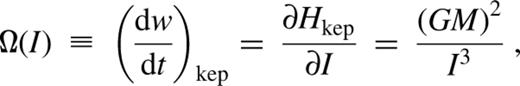
When there is a separation of time-scales, and one is interested in the slow evolution, it makes sense to average over high-frequency variations; thus, time averages of physical quantities are equated to their space averages, an idea that has its roots in the works of Laplace, Lagrange and Gauss on planetary dynamics. Orbit-averaging has also been applied to study the evolution of the orbits of comets, perturbed by the Galactic tidal field (Heisler and Tremaine 1986). The straightforward way to achieve this is to express the problem in appropriate action—angle variables, identify the fast and (the two) slow angles, and integrate over the fast angle. Then the conjugate (fast) action is predicted to have no secular evolution. Laplace did this for the solar system, and concluded that the semimajor axes of the Keplerian ellipses of the planets do not evolve secularly. However, this is a reasonable approximation for the solar system only over times of order 104 yr. A major contribution to limiting the validity of averaging over orbital motions of the planets is mean motion resonances (i.e. ‘fast—fast’ resonances). A natural worry is whether a similar phenomenon will afflict stellar dynamics in galactic nuclei. Let us consider nuclear star clusters in the collisionless limit, when there are an infinite number of stars contributing to a total finite mass for the cluster. Then each stellar orbit can be thought of as being smoothly populated with stars. The gravitational force exerted by such an orbit on a test star will not display time variation on the orbital time-scale (which would have been obtained in the planetary case, when only one planet populates the orbit). Thus we expect no mean motion resonances in star clusters around nuclear BHs.2 Resonances between fast and slow motions can be important for orbits with semimajor axes ∼rh, and will stand in the way of this naive averaging procedure. Such resonances are the seeds of chaos, which we explore in Section 5.
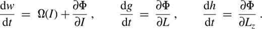
For razor—thin discs, motion is confined to the z=0 plane. Any Φ(x,y) has the two slow integrals of motion, I and Φ. Hence the slow dynamics for two-dimensional potentials, however non-axisymmetric or lopsided, is integrable, and a straightforward classification of orbits is possible.
for axisymmetric Φ in three dimensions, Lz is an exact integral of motion (since Φ is independent of h). We now have three integrals of motion (Lz, I and Φ), and the slow dynamics is again fully integrable.
In three dimensions, when Φ has no symmetry whatsoever, we still have the integrals I and Φ. The slow motion can be chaotic, but it is clear that the chaos is limited.
2.1 Adiabatic growth of the BH
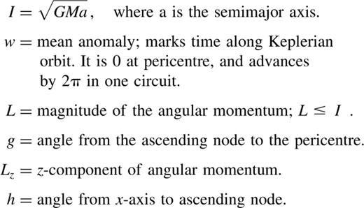
Averaging is also applicable to time-dependent perturbations, Φ(r,t), when the time variations are slower than the orbital times; as before, I=√GMa is a quasi-invariant. In some scenarios of the formation and subsequent growth of the BH, its mass increases adiabatically (Peebles 1972; Young 1980); conservation of I implies that the semimajor axis shrinks in proportion to the growth of M. When the growth time is also much longer than the precessional time-scales, additional (adiabatic) invariants might arise. These will, in general, be related to the actions corresponding to precessional degrees of freedom (L,Lz,g,h). We again consider cases with different spatial symmetry.
for razor-thin discs, the conserved actions are I and L dg, where the integral is performed at a fixed time, over one cycle of motion in the L-g plane.
for three-dimensional, axisymmetric cases, in addition to I and L dg, we have Lz as an exactly conserved quantity.
for configurations that have no spatial symmetry, I is in general the only conserved quantity, since resonances or precessional chaos might destroy the other adiabatic invariants.
It is difficult to make further progress without taking into account the self-consistent evolution of the cluster potential.
2.2 Slow planar dynamics

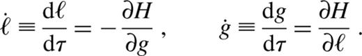
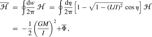
In fact, much of the qualitative picture of the orbit families can be gleaned by studying the contour plot of H in the (g,ℓ) plane (for some value of the constant I).
2.3 A family of planar model potentials
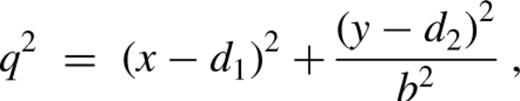
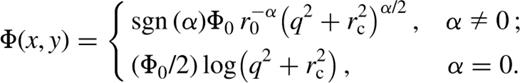
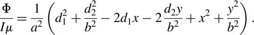
The potentials depend on the five structural parameters, (d,rc,b2,c2,α ), and a magnitude parameter (Φ0r0−α). The potentials are centred at a point that is displaced from the BH by d≡(d1,d2). Potential isocontours have a core of radius rc, and constant axis ratio, b. The exponent α is a measure of the potential gradient across the contours; we require 2≥α>−1, a range that includes homogeneous cores as well as very centrally concentrated mass distributions. The potentials are lopsided for non-zero d, and are cuspy when rc=0. When both d=0 and rc=0, the dynamics itself is scale-free, so we may set a=1 . Lopsided potentials are not scale-free, even when rc=0; this is because the lopsidedness sets a scale (d). The magnitude (Φ0r0−α) measures the slowness of the dynamics. Specifically, we choose units such that μ=(Φ0aα/Ir0α)=(Φ0aα/√GMa r0α). As discussed above, the small parameter is (μ/Ω)∝a(1+α); as α>−1, averaging is a very good approximation for small a.
3 Planar Harmonic Perturbations
The slow dynamics of harmonic perturbations, for which α=2, can be studied exactly for arbitrary non-axisymmetry, and lopsidedness. Pfenniger & de Zeeuw (1989) studied stellar orbits in the combined fields of a point mass, and a non-axisymmetric harmonic potential. For small energies, they report that the orbits are essentially regular orbits in the Kepler potential of the point mass. As we demonstrate in this section, this is not quite true; the lenses and loops that emerge from our investigations are only locally Keplerian. They are better described as precessing and deforming Keplerian ellipses. They point out (correctly) the chaos that occurs for orbits with a∼rh, and discuss orbits of much higher energies. These are the orbits that will determine the overall shape of a galaxy, and they make the interesting point that, if the x and y frequencies of the harmonic potential are commensurate, then the high energy orbits will tend to stay well away from the centre, and hence avoid being strongly perturbed by the BH. We do not discuss their work any further, because our interest is dynamics within rh.
3.1 Centred harmonic perturbation: d1=d2=0
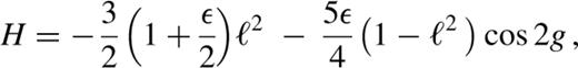
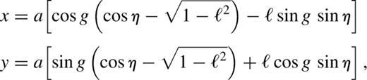
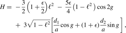
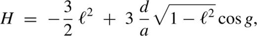
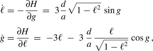
When ε=0, the full Hamiltonian is axisymmetric and the angular momentum is an exactly conserved quantity. The orbits are the rosette-like figures given in standard text books on classical mechanics. The averaged description, of course, coincides with this picture; H=−3ℓ2/2 , the isocontours of which are simply lines of constant ℓ in the (g,ℓ) plane. These loop orbits are now viewed as Keplerian ellipses that precess at a rate, ġ=−3ℓ .
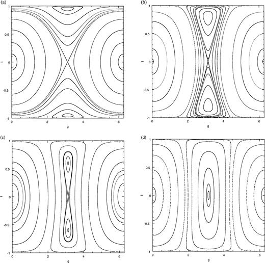
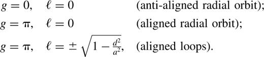
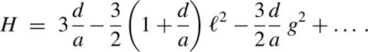
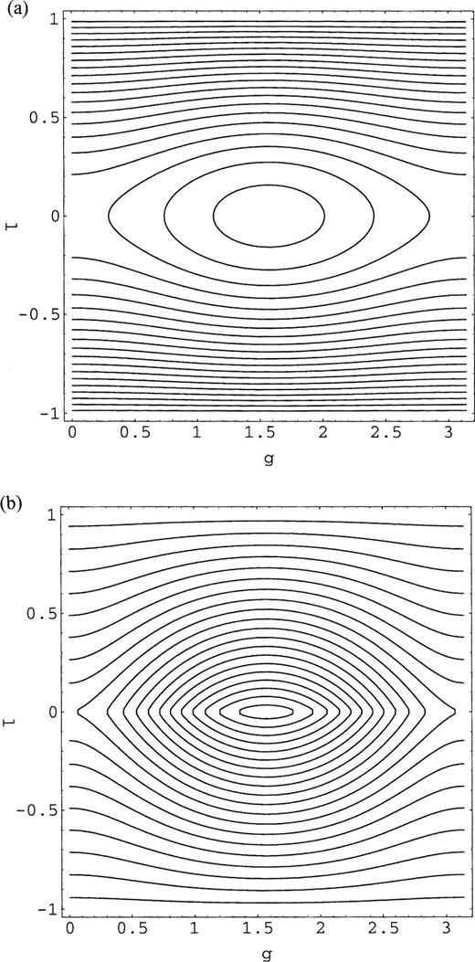
When ε≠0, the non-axisymmetry gives birth to a new family of orbits, the lenses. Fig. 1(a) shows contour plots of H for the case ε=0.25, for which the isocontours of the perturbation have axis ratio b≃0.9 . The lenses are parented by the short-axis orbits, which appear as the stable fixed points located at (/2,0) and (3/2,0). Fig. 1(b) shows a lens orbit (for H=−0.13); ℓ oscillates about zero, whereas g librates about the short axis. When g=/2, it is maximally round, and when the pericentre reaches its maximum deviation from the short axis, the lens elongates to a line (‘radial orbit’); its angular momentum now switches sign, and the orbit returns to maximal roundness at g=/2, but with the opposite sign of ℓ . Unlike lenses, loops have a definite sign for ℓ, and g circulates through 2 in one period. The loop in Fig. 1(c) is a deformed rosette that spends somewhat more time near the long-axis, as it circulates around the origin. The unstable fixed points at (0,0) and (,0) correspond to the long axis orbits. Loops are separated from lenses by the separatrix that straddles the unstable fixed points. The separatrix orbit, as well as the loops and lenses that are close to it, spend a lot of time in the vicinity of the long axis. As ε increases, lenses occupy an increasingly larger fraction of phase space (see Fig. 1d).
Planar, centred, harmonic perturbation: (a) isocontours of H in the (g,ℓ) plane for ε=0.25, (b) a lens orbit in real space corresponding to H=−0.13, (c) a loop orbit in real space corresponding to H=−0.47, (d) isocontours of H in the (g,ℓ) plane for ε=1.
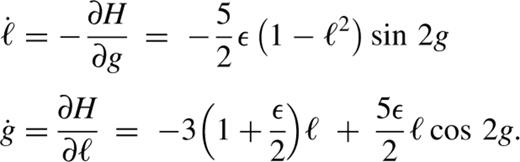
When g=nπ, equations (26) imply that ℓ̇=0 and ġ=(ε−3)ℓ. Thus, when ε=3, g=0, are lines of fixed points in the (g,ℓ) plane. In fact, when ε=3, the region occupied by the short-axis lenses has expanded to its fullest, squeezing the loops out of existence. This value of ε corresponds to an axis ratio of two (for the isocontours of the harmonic perturbation), a case for which the full (unaveraged) Hamiltonian is exactly integrable (see Appendix A for details). For ε>3, loops are completely absent, and all of phase space is populated by lenses (see Fig. 2a). The long-axis orbits now become stable and parent families of long-axis lenses, one of which is shown in Fig. 2b. We can demonstrate this change in stability of the long-axis orbit, by expanding the H of equation (24) to lowest order about the fixed point (0,0):
Planar, centred, harmonic perturbation: (a) isocontours of H for ε=5.0, (b) a long-axis lens orbit, for H=−6.0.

The coefficients of both ℓ2 and (Δg)2 have the same sign, so the short-axis orbit is always stable.
3.2 Lopsided harmonic perturbation: d1?0, d2=0, e=0
The panels in Fig. 3 show the dependence of the isocontours of H on lopsidedness. Changes in the topology of isocontours occur when d/a crosses 0.5 (Figs 3a and b), and again when d/a crosses unity (Figs 3c and d). This behaviour is best understood by following the location and stability of the fixed points. The equations of motion are,
Isocontours of H for planar, lopsided, harmonic perturbation: (a) d=0.3a, (b) d=0.6a, (c) d=0.8a, (d) d=1.5a.
The coefficients of ℓ2 and g2 have the same sign, so the fixed point is stable.

When d<a, the coefficients of ℓ2 and (Δg)2 have opposite signs (fixed point unstable), but have the same sign for d>a (fixed point stable). Hence there are three kinds of fixed points:
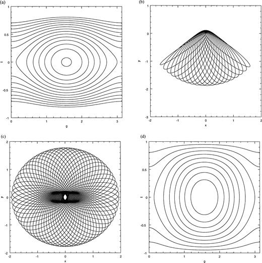
The anti-aligned radial orbit is stable for all d/a. This parents a family of anti-aligned lenses (see Fig. 4a).
The aligned radial orbits are stable when d>a, and parents a family of aligned lenses (see Fig. 4d).
The aligned loop orbits are stable when d<a. These parent a family of librating loops, to be discussed in some detail in the following.
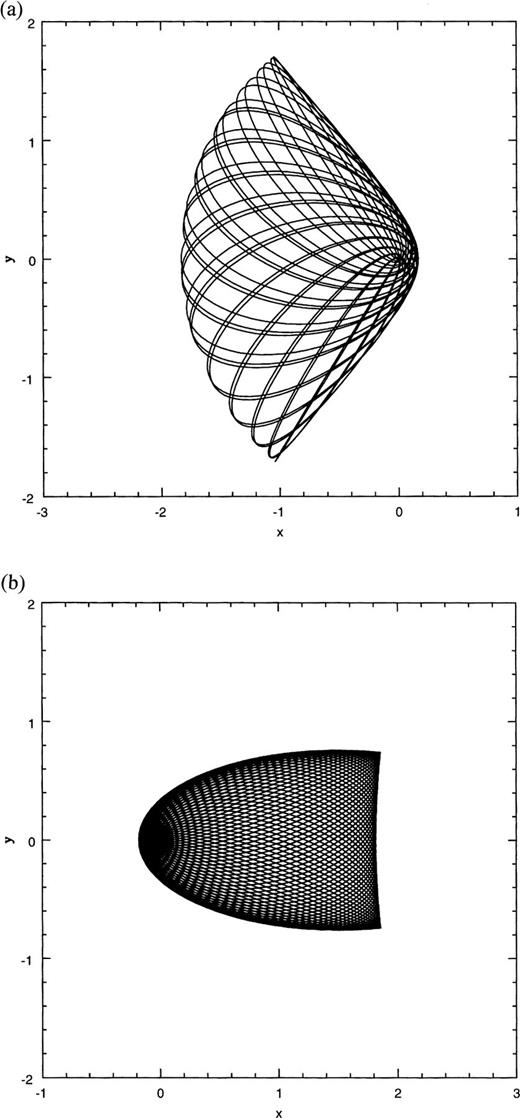
Lens orbits for the planar, lopsided, harmonic perturbation: (a) an anti-aligned lens orbit for a=1, d=0.5, (b) an aligned lens orbit for a=1, d=1.5.
There are no orbits that correspond to anti-aligned loops.
3.3 Possible applications to lopsided galactic nuclei
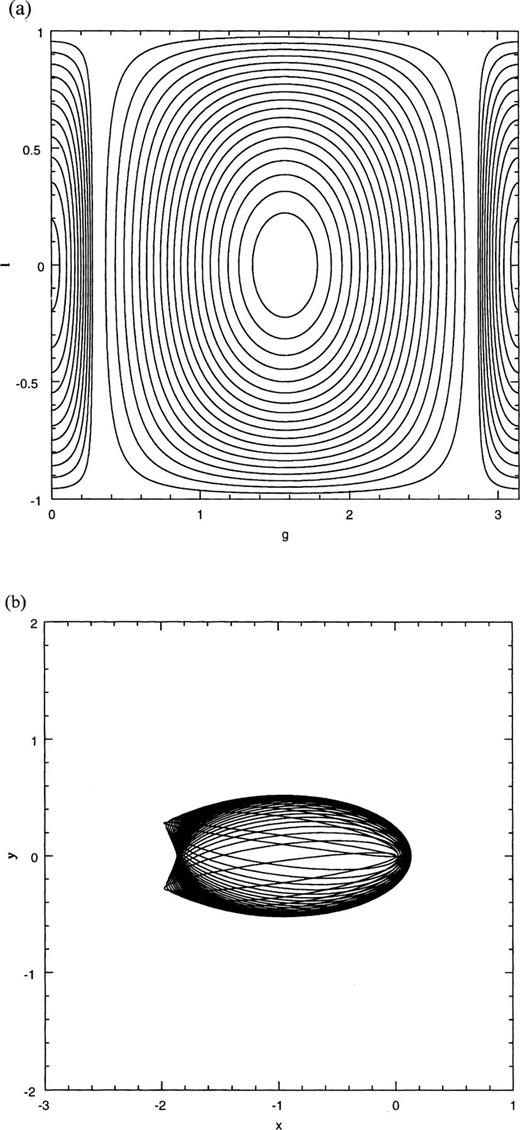
The aligned loops (which are fixed points of the slow dynamics) have constant angular momentum; ℓ is positive (negative) for anti-clockwise (clockwise) motion of the particle on its Keplerian ellipse. Their eccentricity, e=d/a , which means that the centres of the ellipses coincide with the centre of the perturbation (the BH is at one of the foci). For a fixed value of d, aligned loops of varying sizes (i.e. a), form a family of concentric, confocal ellipses. Not only can stars be placed on such orbits, but being a non-intersecting family, such nested ellipses can also be the streamlines of gas flows. Fig. 5(a) shows one such representative set of aligned loops. Stable oscillations about these fixed-point orbits allows ℓ to oscillate, while preserving a definite ± sign. Unlike the circulating loops of the centred perturbation (see Fig. 1c), g for one of these librating loops oscillates about its mean value of (see Fig. 5b).
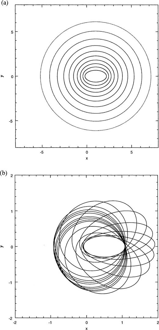
Loop orbits for the planar, lopsided, harmonic perturbation: (a) a set of aligned loops when d=1. The ten nested ellipses have a=1.2,(1.2)2,…,(1.2)10≃6.19, (b) a librating loop for d=0.5, a=1, for which ℓ fluctuates between 0.4 and 0.97.
Tremaine (1995) has suggested that the nucleus of M31 is an eccentric disc in which stars move on nearly Keplerian orbits around a massive BH. In his model, the location of the BH coincides with the fainter (brightness) peak, P2, and the brighter peak, P1, is the apoapsis region of the Keplerian ellipses. If we imagine that the lopsided harmonic perturbation mocks self-gravity, our toy model suggests that the orbits such as our aligned loops (and their progeny, the librating loops) might form the backbone of star clusters such as Tremaine's eccentric discs.
4 Perturbations gor General α
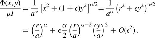
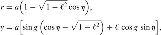
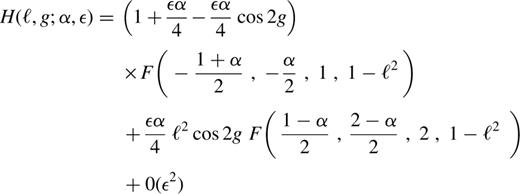
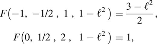

Fig. 6(a) shows the isocontours of this Hamiltonian (α=1) for ε=0.1 ; as may be seen, these are similar to those of Fig. 1(a). Keeping ε small, we can vary α from −1 to 2. Fig. 6(b) shows the isocontours for α=−0.9; again the overall structure is unchanged. Hence we conclude that, for small ε, the orbital structure is independent of α in the range (−1,2), with loops and short-axis lenses broadly similar to those in Figs 1b and c.
Isocontours of H for ε=0.1 (accurate to first order in ε): (a) α=1, (b) α=−0.9.
5 The Limits of Averaging
The averaged Hamiltonian is an accurate proxy for the full Hamiltonian when the orbital period is much shorter than the period of precession of periapse. Such is mostly the case for orbits that reside within the sphere of influence of the BH. However, as one moves outwards, the influence of the perturbations relative to the pull of the BH increases and the mismatch in frequencies decreases, thereby invalidating the averaging procedure. In practice, the breakdown occurs at resonances between orbital and precessional motion, and is responsible for the emergence of minor orbit families such as the ones discussed by Gerhard & Binney (1985, hereafter GB) and Miralda-Escudé and Schwarzschild (1989, hereafter MES).
MES studied the scale-free case throroughly. The phase space is divided between orbits with a definite sense of circulation (librating non-aligned loops and rosettes) and those with no definite sense of circulation. The latter are broken into resonant orbit families: banana, fish, pretzel… etc. The resonances are between the orbital period of the star and the period of precession of its pericentre. The banana for instance, performs two orbital revolutions in the time it takes its pericentre to precess once. Such resonances are naturally missed by the averaged Hamiltonian, which assumes that the orbital period is much faster than the precessional period [see Touma & Tremaine (1997) for a discussion of the averaged Hamiltonian].
We now place a BH at the origin and study the restructuring of orbits that occurs. MES did introduce a BH but did not show any surface of section. They presented samples of high-energy orbits, including some regular ones. The BH radius of influence is given by rh=GM/vL2. We measure distance in units of rh, and look at sections of increasing energy. The energy is that of an orbit with zero velocity started on the x-axis, with x=frh, f=0.4,2.0,4.0.
Within rh (Fig. 7a), the phase space is occupied by two main families of regular orbits: short axis lenses and loops. The lenses appear naturally in the integrable cusps with BHs presented in Sridhar and Touma (1997). The apparent integrability of the motion is consistent with the validity of averaging at distances where the motion is dominated by the BH. The phase space of the corresponding averaged Hamiltonian has not been described in this paper, but it hardly differs from the averaged dynamics of centred harmonic perturbations discussed above (this should be obvious from the results of Section 4). As one moves out in radius past rh (Fig. 7b), resonances become stronger, and a layer of stochastic motion develops near the separatrix. A torus has broken up into a chain of islands. The corresponding resonant periodic orbit, the bow-tie, is shown in Fig. 7c. Further away from the BH (Fig. 7d), the short-axis radial orbit becomes unstable, and bananas are born, together with other resonant orbit families, which overlap and lead to large-scale chaos where once the regular lens orbits lived.
Dynamics in the potential of a black hole perturbed by a logarithmic potential with b=0.9: (a) Section on energy surface with zero velocity orbit y=0 and x=0.8rh; (b) similar section but with x=2.0rh ; (c) periodic orbit at the centre of the chain of islands seen in (b); (d) section on energy surface with zero velocity orbit y=0 and x=4.0rh.
GB studied the logarithmic potential with core and BH. They were mostly interested in energetic orbits far outside rh, and they find that resonant orbit families and stochastic orbits dominate the phase space. When commenting on dynamics inside rh, they just mention that most orbits are loops which, as we now know, is incomplete. In fact, within rh, the dynamics is accurately described by the integrable, orbit-averaged Hamiltonian; the phase space is regular with mainly short-axis lenses and loops. As one moves outside the sphere of influence, lenses and loops break down into resonant orbit families, which get stronger, overlap and lead to stochastic orbits. The short-axis radial orbit goes unstable and regular lens orbits disappear, as the region within the separatrix is practically engulfed by a single stochastic orbit. GB described stochasticity in terms of the scattering of box orbits by the central cusp and BH. Here, stochasticity emerges with the gradual sacrifice of regular lens orbits to strong overlapping resonances as we move away from the BH.
6 Discussion
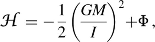
In this paper we have introduced an averaging technique into the study of star clusters around massive BHs at the centres of galaxies. The dynamics of these clusters is governed by the combined gravitational potential of the central BH and the cluster itself. Within the sphere of influence (rh) of the BH, the cluster potential is a small, yet non-negligible perturbation. Orbits that are confined within rh may be viewed as slowly precessing (and deforming) Keplerian ellipses. We have shown that these orbits possess a quasi-integral of motion, in addition to the energy integral; this nearly conserved quantity is I=√GMa, where M is the mass of the BH, and a is the semimajor axis of the orbit (when M is constant, the semimajor axis is nearly conserved). The quasi-integral arises because the Keplerian orbital frequency is much larger than the frequencies of precessional motions. Taking advantage of this mismatch in frequencies, we averaged over an orbital period, to obtain a reduced dynamics of slow, precessional motions, wherein I appears as a full-fledged integral of motion.
The building of self-consistent stellar models for systems with low spatial symmetry (such as the central regions of M31 and NGC 4486B, which are known to possess double nuclei) surely requires the existence of more than one integral of motion. We now have in hand two integrals of motion — the energy and the semimajor axis — that may be used to construct dynamical models for the centres of galaxies like M31 and NGC 4486B. Let us verify that the conditions required for the averaging to apply are met in these two cases.
(1) M31 probably has a central BH of mass ∼6×10⁷ M⊙. For velocity dispersion ∼160 km s−1, rh∼10 pc (∼3 arcsec). The double nuclei are separated by ∼0.5 arcsec, and much of the nuclear disc itself appears to be within rh. Furthermore, within 1 arcsec, the masses of the disc and the bulge are only 16 and 2 per cent of the mass of the BH, respectively (see Tremaine 1995). Within rh, the gravitational potentials of the disc and bulge are small, but non-negligible perturbations to the potential of the BH; indeed, this is a situation that is ripe for the application of the averaging technique! In Sections 3.2 and 3.3, we considered orbits in a toy model of a lopsided perturbation, and discovered that there is a very interesting class of loop orbits, in which the orbits are elongated in the same sense as the perturbation. The existence of these aligned loop orbits is an encouraging sign that Tremaine's (1995) eccentric disc can be realized as a self-consistent model.
(2) NGC 4486B (a low luminosity E1 companion of M87) also has a double nucleus separated by 0.15 arcsec (Lauer et al. 1996). There seems to be some evidence for a central BH of mass ∼9×10⁸ M⊙ (Kormendy et al. 1997). For a velocity dispersion ∼175 km s−1, and an assumed distance to NGC 4486B of 16 Mpc, we estimate that rh∼1.6 arcsec, a length scale that is not only larger than the separation between the nuclear peaks, but also nearly fifteen times larger than the best resolution obtainable with the HST; hence the averaging technique may be expected to be useful here too. Kormendy et al. (1997) suggest that the double nucleus might arise from a stellar distribution similar to Tremaine's (1995) disc. However, as Lauer et al. (1996) note, there are differences from the case of M31, and even the evidence for a massive BH is less certain.
A fundamental result of this paper is that the presence of a massive BH enforces a certain degree of integrability within its sphere of influence, and this happens because of the existence of the secular invariant, I. Even without detailed knowledge of the (perturbing cluster) potential, we were able to note that slow dynamics in (i) razor-thin discs is fully integrable because the problem is two-dimensional, (ii) any axisymmetric potential is fully integrable (note that axisymmetry allows for lopsidedness), and (iii) a potential with no spatial symmetry whatsoever still conserves two integrals, so that any precessional chaos must be highly limited in nature.
When the potential is time-dependent, but with variations occurring over times longer than the orbital times, averaging is still applicable. We discussed the case of the adiabatic growth of the BH. Another case of slow time variation comes to mind: this is the ‘resonant relaxation’ of Rauch and Tremaine (1996), a process that relies on two-body encounters between stars. The time-scales are typically much longer than orbital times, so averaging applies, and the stars in their courses may be treated as elliptical rings. Over certain time-scales (shorter than the classical two-body relaxation times), the semimajor axes of all the stars are approximately constant, whereas torques between the rings exchange angular momentum. As the authors note, this can lead to a situation in which some regions of nuclear star clusters are relaxed in angular momentum, but not in energy.
We introduced a family of model planar potentials that allow for a range of cusp slopes (α), non-axisymmetry and lopsidedness, with a view to classification of orbit families. For the harmonic case (α=2), we showed that centred non-axisymmetric perturbations support two main families of orbits: short-axis lenses and loops. Lenses were introduced in Sridhar & Touma (1997) and should be recognized as an essential feature of regular motion around BHs. They have zero average angular momentum and fill out lens-shaped regions in configuration space. The loops are the familiar rosettes of slightly perturbed Keplerian motion. We explored the consequences of lopsidedness and identified a family of (resonant) aligned loops, the elongation of which is in the same sense as the lopsidedness.
When α≠2, the case of small non-axisymmetry (ε≪1) is analytically tractable. The qualitative nature of the orbits (lenses and loops) appears to be insensitive to α. This is probably because the force exerted on a star due to the perturbing potential — even when it becomes infinitely large at the centre — is overwhelmed by the force due to the BH. If such is the case for larger non-axisymmetry, then our explorations of the harmonic case provide a sketch of the possible orbit families in razor-thin discs around massive BHs. Whether the qualitative nature of dynamics around BHs is indeed independent of the steepness of the cusp in density is an unsolved problem, but one that is tractable by methods such as our averaging technique.
Averaging is, of course, valid as long as we are far away from resonances between the orbital period and the periods of apsidal or nodal precession. We showed, numerically, that such a condition is indeed satisfied for r<rh, but breaks down outside. Orbits which take a star far outside rh may be expected to be chaotic [cf. Gerhard & Binney (1985); Merritt (1997)]. Central BHs and strong cusps might force the main body of an elliptical galaxy to evolve towards axisymmetry. However, as we have argued in this paper, the central regions of galaxies might stubbornly persist with their striking variety of non-axisymmetric features.
Acknowledgments
We thank the Raman Research Institute and the Indian Railways for their hospitality while this work was in progress. JT wishes to thank IUCAA for support and hospitality at Pune, as well as acknowledge the support of the Harlan Smith Fellowship under NASA grant NAGW 1477.
References
It should be noted that σ itself is often not independent of distance from the BH. In this case, σ should be taken as the dispersion at r=rh, which results in an equation wherein rh is the unknown quantity to be solved for. Perhaps a better estimate of the sphere of influence of the BH is the radius at which the mass of the cluster equals the mass of the BH.
Of course, clusters might have as few as 106 stars, so that each orbit is not quite smoothly populated with stars. Hence there can be some discreteness noise, which would make the system somewhat collisional.
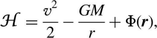
It is unfortunate that the notation employed by planetary dynamicists overlaps so heavily with those commonly used by galactic dynamicists for other physical quantities. Our notation is non-standard, but we hope that it minimizes confusion.
h is, of course, exactly conserved, but this does not give us any extra conserved quantities after averaging.
In the lopsided cases, the potential exerts a force on the BH, so we should imagine that the BH is ‘nailed’ down. It is possible to improve the situation by including cubic and higher order terms in the potential, but at the cost of considerably more complexity. We decided to forgo this luxury, since our primary goal in this paper is to pick out interesting orbits.
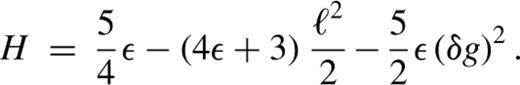
A term, [(5/2)+(5ε/4)+(d1/a)2+(1+ε)(d2/a)2 ], has been dropped in the slow Hamiltonian, because it is does not contribute to slow dynamics.
For α=2, equation (44) reduces to equation (24), which happens to be an exact expression, because terms of O(ε2) are identically zero for this case.
Appendix
Appendix A: The Case ε=3

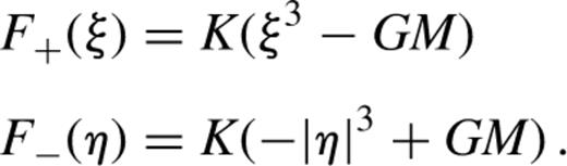
This form is that of a separable, Stäckel potential in parabolic coordinates that supports integrable motion.
Appendix B: Derivation of Equation (25)

