


ABSTRACT
We present the results of two years of radio and X-ray monitoring of the magnetar XTE J1810 − 197 since the radio re-activation in late 2018. Single pulse analysis of radio observations from the Lovell and MkII telescopes at 1564 MHz and the Effelsberg telescope at 6 GHz has resulted in the detection of a total of 91 giant pulses (GPs) between MJDs 58858 and 59117. These GPs appear to be confined to two specific phase ranges (0.473 ≤ ϕ ≤ 0.502 and 0.541 ≤ ϕ ≤ 0.567). We also observe that the first detection of GP emission corresponds to a minimum in the spin-down rate. Simultaneous radio and X-ray observations were performed on MJDs 59009 and 59096. The 0.5–10 keV X-ray spectrum from NICER is well characterized by a two-component blackbody model that can be interpreted as two hot spots on the polar cap of the neutron star. The blackbody temperature decreases with time, consistent with the previous outburst, while the change in the pulsed fraction does not follow the same trend as was seen in the previous outburst. The radio and X-ray flux of XTE J1810 − 197 are correlated during the initial phase of the outburst (MJD 58450 – MJD 58550) and an increase in the radio flux is observed later that may be correlated to the onset of GPs. We argue that the disparity in the evolution of the current outburst compared to the previous one can be attributed to a change in geometry of the neutron star.
1 INTRODUCTION
Magnetars are an extreme class of young, slowly rotating (P ≈ 1–12 s) neutron stars that possess high surface magnetic fields (B ≈ 1013–1015 G) (e.g. Kaspi & Beloborodov 2017a). They exhibit striking variability in their X-ray and soft gamma-ray energies, powered by their decaying magnetic fields (Duncan & Thompson 1992). This variability often manifests itself as common, millisecond-duration bursts, to rarer, bright month-long outbursts, which comprise many of the shorter bursts and a long tail or afterglow (e.g. Kaspi & Beloborodov 2017a). Of the 25 confirmed magnetars,1 only 5 have been detected to pulse in the radio (Camilo et al. 2006, 2007a; Levin et al. 2010; Eatough et al. 2013; Champion et al. 2020). The radio single pulses exhibit extraordinary spectral and temporal phenomenology (Kramer et al. 2007; Camilo et al. 2007b; Serylak et al. 2009; Desvignes et al. 2018), and have recently been suggested as possible progenitors to the enigmatic fast radio bursts (FRBs; Mereghetti et al. 2020; Pearlman et al. 2020).
The magnetar XTE J1810 − 197 was serendipitously discovered in 2003 by the Rossi X-Ray Timing Explorer (RXTE; Ibrahim et al. 2004). Subsequent X-ray follow-up of the source revealed a 5.75 s period, confirming it as an energetic neutron star with a measured magnetic field of 2.1 × 10¹⁴ G. It was later found to be associated with a radio source in the VLA MAGPIS survey at 1.4 GHz in 2005 (Halpern et al. 2005). Observations by Camilo et al. (2006) resulted in the first detection of pulsed radio emission from a magnetar with a dispersion measure (DM) of 178 pc cm−3. Since then, the magnetar has been extensively monitored by both ground and space-based telescopes (e.g. Camilo et al. 2007b; Pintore et al. 2018; Gotthelf et al. 2019a; Torne et al. 2020). Investigations of the radio polarization properties and flux densities has indicated dramatic variations in the polarization position angle over time, and a flat spectral index (Kramer et al. 2007; Dai et al. 2019). The average radio flux density and X-ray flux decreased in the 10 months following the discovery and remained stable for the next ∼2 yr before eventually disappearing towards the end of 2008 (Camilo et al. 2016). The magnetar was then in quiescence until the end of 2018 when it exhibited another large X-ray flare (Gotthelf et al. 2019b) coinciding with the onset of radio emission (Lyne et al. 2018). The source has been continuously monitored in the radio and X-ray, since reactivation with strong pulsations detected at both wavelengths (Desvignes et al. 2018; Joshi et al. 2018; Dai et al. 2019; Lower et al. 2020b). Similar to the 2006 outburst (Camilo et al. 2006; Serylak et al. 2009), the single pulses seen in the current outburst also exhibit ‘spiky’ millisecond-width pulses in the radio (Dai et al. 2019). Maan et al. (2019) investigate this spiky emission and report on its similarities to those of the giant micropulses, thereby suggesting a possible link in the underlying emission mechanisms. The recent discovery of millisecond-duration radio pulses (CHIME/FRB Collaboration et al. 2020a; Bochenek et al. 2020) from the magnetar SGR 1935 + 2154 in our own Galaxy coincident with high-energy emission in the X-ray and gamma-rays (Mereghetti et al. 2020; Zhang et al. 2020) indicates that at least some magnetars produce FRBs.
The Lovell and Mark II (MkII) telescopes at the Jodrell Bank Observatory (JBO) has been regularly monitoring the magnetar as part of a timing programme (Lyne et al. 2018). Fortuitously, the magnetar has also been extensively monitored at soft X-ray wavelengths with the Neutron Star Interior Composition Explorer (NICER) instrument on board the International Space Station (Gendreau et al. 2016). In this paper, we report on the long-term timing and single-pulse analysis of XTE J1810 − 197 with the JBO and Effelsberg telescopes and quasi-simultaneous X-ray analysis with the NICER instrument. Following the detection of giant pulse (GP) like emission in the radio, we performed simultaneous observations on 2020 June 9 and 2020 September 4 in the radio and X-rays with the Effelsberg and MkII telescopes, and the NICER telescope, respectively. We present the results of the simultaneous observations and investigate the existence of quasi-periodicity in the radio single pulses. In Section 2, we present the radio and X-ray observations of XTE J1810 − 197. The analysis and results of these observations are presented in Section 4. We discuss possible implications of our findings in Section 6 and draw our conclusions in Section 7.
2 RADIO OBSERVATIONS AND DATA REDUCTION
2.1 Lovell and Mark II
As detailed in Levin et al. (2019), the magnetar XTE J1810 − 197 has been monitored since the beginning of 2009 using a combination of the 76-m Lovell telescope and the 26-m Mark II (MkII) telescope at JBO. The total intensity data for the Lovell and MkII telescopes were divided into sub-bands using a ROACH board (Bassa et al. 2016) and then channelized in real-time using the digifil algorithm from the dspsr software package (van Straten & Bailes 2011). The resulting filterbanks were recorded with the Apollo backend instrument at a time resolution of 256 |$\mu$|s covering a total bandwidth of 336 MHz centred at 1564 MHz. The data are divided into 672 frequency channels during acquisition. Each of the Lovell observations varied from 10 to 30 min in duration, while the MkII observations were between 10 min and 1 h long. For all observations, single pulse archives were created offline using the dspsr software package with an ephemeris obtained from the joint timing analysis of all the JBO and Effelsberg data, and dedispersed to a DM of 178 |${\rm pc \, cm^{-3}}$|. Since our data were affected by radio frequency interference (RFI), we used a combination of the clfd2 package described in Morello et al. (2019) and the Inter-Quartile Range Mitigation (IQRM) algorithm3 to flag the channels with the most prominent RFI. Additionally, the data were visually inspected and manually cleaned using PSRCHIVE4 tools. An integrated pulse profile was created using the cleaned pulses, and folded and de-dispersed using the same ephemeris and DM as the single pulses.
2.2 Effelsberg
The 100-m Effelsberg radio telescope has also been monitoring the source, since its outburst in December 2018. The observations presented here were performed using the S45mm single pixel receiver tuned at a central frequency of 6 GHz with a system equivalent flux density of 25 Jy averaged across the 4 GHz band. The data were recorded in full Stokes mode using two ROACH2 backends, splitting the band into 4096 frequency channels, and have a time resolution of 131 |$\mu$|s. Similar to the Lovell and MkII data analysis, the Effelsberg psrfits format search-mode data were processed for single pulses using dspsr and the same ephemeris as used for the Lovell and MkII data processing. Initial RFI mitigation was performed using the clfd package and further visual inspection and manual cleaning was carried out later using standard PSRCHIVE pulsar packages. The Effelsberg observations reported in this paper range from 11 min to 1 h in duration. Simultaneous observations were undertaken with the MkII and Effelsberg telescopes on 2020 June 9 and 2020 September 4.
3 X-RAY OBSERVATIONS AND DATA REDUCTION
Since the outburst in 2018, the NICER X-ray telescope has been monitoring XTE J1810 − 197, providing a high cadence X-ray data set over a span of more than 1.5 yr since the onset of the outburst. NICER provides fast-timing spectroscopy observations with a large effective area in soft X-rays (0.2–12 keV) as an external payload on the International Space Station (Gendreau et al. 2016). After the onset of another period of bright radio activity from the magnetar in early 2020, we submitted a Target of Opportunity (ToO) proposal to observe XTE J1810 − 197 simultaneously at X-ray and radio wavelengths to investigate any correlation in the X-ray and the radio light curves. In total, we were awarded three observations, each spanning 2 ks on the source. For the first two observing sessions (2020 June 6 and 9), we observed simultaneously with the 26-m MkII telescope at 1564 MHz. The observations on 2020 June 9 were also shadowed by 6.0 GHz observations with the 100-m Effelsberg telescope. The third observing session on 2020 September 4 was shadowed by the MkII telescope. We note that the X-ray observations did not overlap with the entire span of the radio observations as continuous observing with NICER is significantly constrained by the orbital period of the International Space Station on which NICER is mounted. Along with the simultaneous observing, we also downloaded the publicly available data on the magnetar from March of 2019 from the HEASARC NICER data archive.5 This resulted in a large X-ray data set on XTE J1810 − 197 with an approximately monthly cadence over the span of 1.5 yr. We do note that there is a gap in the X-ray monitoring of the source from 2019 November until 2020 March as the source was at very low Sun angles (Sun constrained).
For calibration and filtering of the data, we used heasoft version 6.25 and nicerdas version 2018-10-07 V005. We applied the standard filtering criteria (excluding events acquired during times of South Atlantic Anomaly passage and with pointing offsets greater than 54 arcsec; including data obtained with Earth elevation angles greater than 30° above the dark limb and 40° above the bright limb). The source was Sun constrained until 2019 February. The observations conducted during 2019 February were severely affected by optical loading of the X-ray detectors of NICER as the angle from the Sun was never above 60°. We used the standard NICERDAS suite nicerl2 to calibrate, filter, and extract good time intervals (GTIs) for all our observations. For each GTI, we extracted the corresponding XTE J1810 − 197 spectrum. For the 2020 June 6, 9 and 2020 September 4 observations, we also extracted the light curves for XTE J1810 − 197 with a time bin size of 1 s. Our choice of a large bin size was to gather sufficient photon counts per pulse phase bin above the noise threshold in order to see any correlations with the radio data. Because NICER consists of non-imaging detectors, the NICER team has developed a space weather-based background model, which estimates spectral contributions from the time-dependent particle background, optical loading from the Sun, and diffuse sky background using a library of observations of ‘blank sky’ fields (K. C. Gendreau et al. in preparation). Using the nibkgestimator tool provided by the NICER team,6 we estimated the background spectrum for each observation segment separately. The lack of any other bright X-ray source in the field of XTE J1810 − 197 excludes the possibility of source confusion when reducing NICER data.
4 RADIO DATA ANALYSIS AND RESULTS
4.1 Profile evolution
The radio profile of XTE J1810 − 197 has undergone considerable changes since 2019 (Levin et al. 2019), exhibiting discrete components which change their relative flux densities with time and frequency. The total intensity profiles from the Lovell and MkII telescopes at 1564 MHz are shown in Fig. 1. Each profile is averaged over 15–20 d. The main pulse profile peak has changed from being flanked by components on either side (MJD 58503), similar to the last few epochs in Levin et al. (2019), to having a precursor component on the left, centred around phase −0.12 periods (MJD 58604). At MJD 58635, the main peak dropped in intensity while the precursor component got brighter. Between MJDs 58720 and 58803 inclusive, the profile underwent a number of changes, transitioning from a two- to a four- to a three-peaked profile. The comparatively lower signal-to-noise ratios (S/Ns) of these profiles are in part because they were obtained using the smaller MkII telescope, which has a sensitivity of about 1/10 of that of the Lovell, and in part because the pulsar flux density was low at that time (see Fig. 17). From MJD 58920, the profile transitioned back to having two-components (but with a much temporally closer post-cursor rather than a precursor), and evolved into a stable single peak after MJD 59077. The smaller data set of higher-frequency observations carried out at Effelsberg also show drastic changes, but the profile components have differing spectra so that approximately contemporaneous Jodrell Bank profiles look quite different. The time alignment of the Jodrell Bank and higher frequency Effelsberg profiles is discussed below.
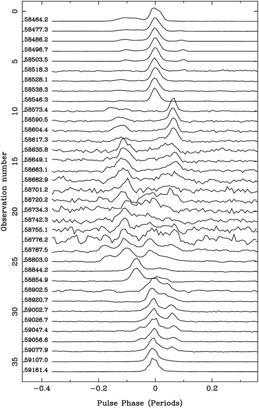
Normalized total intensity profiles for observations performed with the Lovell and MkII telescopes at 1564 MHz between 2018 and 2021. The profiles with the comparatively poor S/N between MJD 58590 and 58776 were carried out using the smaller MkII telescope (see Section 4.1). Each profile has been averaged over 15–20 elapsed days. Phase zero corresponds to the position of the high-frequency component referred to in the text.
4.2 Timing analysis
A phase-coherent timing solution was obtained using a combination of the Lovell, MkII and Effelsberg data spanning ∼2 yr from the start of the recent outburst in 2018 December. Times of arrival (ToAs) were generated by cross-correlating the integrated profile for each MJD with a standard profile using standard PSRCHIVE pulsar timing tools. This process was more difficult than usual because of the profile changes described above and seen in Fig. 1. For the Jodrell Bank data, multiple standard profiles were created by aligning and integrating observations from MJDs 58460 to 59210. Different standard profiles were adopted when significant changes in profile shape occurred. The changes mostly occurred abruptly, without any immediate change in phase drift rate across the event, relative to a pre-event ephemeris. A new standard profile was adopted and adjusted in phase so as to cause no discontinuous step in timing residuals. This process was repeated at each of the four major changes, resulting in five standard profiles, which are all aligned with the phase of the intense dominant component present at around MJD 58500.
Inspection of the multifrequency data set shows that this dominant component has a very different spectrum from other components and is even more dominant at higher frequencies, so that it is always present during the Effelsberg observations and nearly always the brightest feature at 6 GHz. ToAs for this feature were obtained using a standard profile which was typical for this component and which was aligned with the dominant component in the standard template for the Jodrell Bank data around MJD 58500. The ToAs were processed using the tempo27 (Hobbs, Edwards & Manchester 2006) software package. In order to investigate the quality and consistency of the timing data, we fitted for the spin frequency (F0) and its first four derivatives, keeping the DM fixed at 178 pc cm−3. We present the results in Table 1. The residuals of the ToAs relative to this model are shown in Fig. 2 and show only smooth variations in rotation. There is no indication of any discontinuities, which might have arisen at changes in standard profile. Additionally, the high-frequency Effelsberg points are satisfactorily consistent with the Jodrell Bank data. It should be noted that the variable nature of the profiles in this source means that the standard profiles are often imperfect matches to the observed profiles, which frequently vary in detail from hour to hour and day to day. Close inspection of the timing residuals indicates a typical rms jitter of about 50 ms or 0.01 in pulse phase, increasing where the pulse is less distinct.
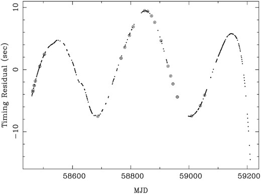
Radio timing residuals for XTE J1810 − 197 relative to the rotation model presented in Table 1. The small number of high-frequency data from Effelsberg are identified by surrounding open circles. The formal errors in the ToAs are less than the size of the symbols.
Timing parameters of XTE J1810 − 197 for the data used in this work.
| Parameter | Value |
|---|---|
| Right ascension (J2000) (hh:mm:ss) | 18:09:51.140 |
| Declination (J2000) (dd:mm:ss) | −19:43:51.200 |
| DM (pc cm−3) | 178 |
| Date range (MJD) | 58460.649106–59210.427533 |
| Epoch of frequency | 58848.5 |
| F0 (Hz) | 0.180445476(12) |
| F1 (Hz s−1) | −2.355(11) × 10−13 |
| F2 (Hz s−2) | 1.58(3) × 10−20 |
| F3 (Hz s−3) | −8.09(14) × 10−28 |
| F4 (Hz s−4) | −1.57(4) × 10−34 |
The timing model derived above suggests that the spin frequency derivative (F1) is changing rapidly, and we have performed a series of stride fits to the data to investigate the evolution of |F1| with time (Fig. 3). Indeed, the spin-down rate, |F1|, varies by a factor of about 5, reaching a minimum around the middle of these observations. The errors in the fitted values reflect the measurement jitter and are usually small compared with most of the structure seen in the figure.
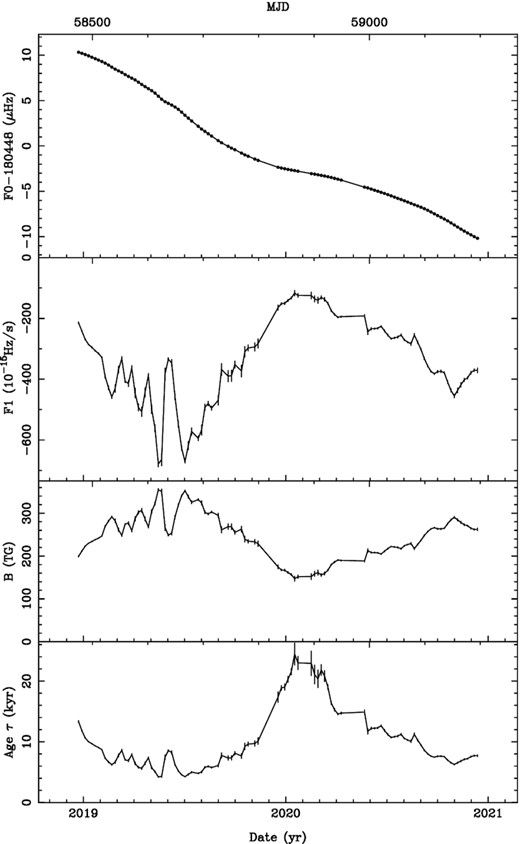
Evolution of the spin frequency (F0), frequency derivative (F1), magnetic field (B|$= 3.2 \times 10^{19}\, \sqrt{P\dot{P}}$|), and characteristic age (|$\tau = P/2\dot{P}$|) as a function of time. Timing fits of F0 and F1 were made to the data over successive 30-d periods, starting at intervals of 10 d, so that adjacent points are not completely independent.
4.3 Spiky giant pulse-like emission
The strongest argument for the presence of a distinctive ‘spiky’ emission is visible in an example pulse stack shown in Fig. 4. Bright, narrow (see Table A1, for values of S/Ns and widths) pulses visible across the whole observing band appear to dominate the emission suggesting that they may have different properties from the rest of the observed emission. Though the pulse stack is dominated by the spiky emission, we note that there is an almost indiscernible background of weak emission in the Effelsberg pulses. We refer to this as ‘normal’ emission throughout the paper. The MkII pulses are however purely dominated by spiky emission and the absence of normal emission can be reconciled by the difference in sensitivities between the Effelsberg and MkII telescopes. Similar to Maan et al. (2019), we examine the possibility of some of the spiky emission being true giant pulses (GPs) by definition (see Sections 4.3.2 and 4.3.1 for more details), by computing the pulse energy distributions. We note that throughout the paper, the Lovell and MkII data are flux calibrated, while we use the flux density values from the radiometer equation for the Effelsberg data.
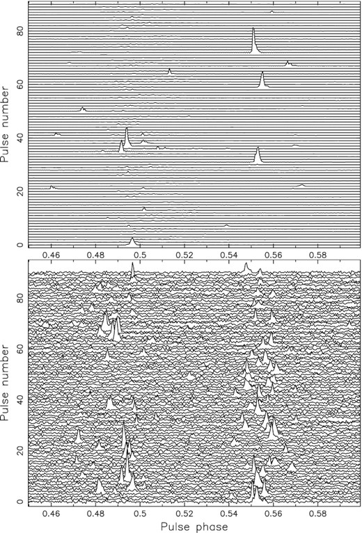
Pulse stack of XTE J1810 − 197 single pulses from simultaneous Effelsberg and MkII observations on MJD 59009. Top panel: Effelsberg single pulses observed at 6 GHz. Bottom panel: MkII single pulses at 1564 MHz.
4.3.1 Pulse energy distributions
We calculate the pulse-energy distributions of XTE J1810 − 197 to compare the observed bright pulses with the GP phenomenon (e.g. Serylak et al. 2009). To do this, we calculate the total single pulse energies and compare them with the average pulse energy. For each individual pulse, we calculated the average flux densities within the on-pulse region after subtracting the baseline noise using psrsalsa8 (Weltevrede 2016). The off-pulse energy was determined in the same way using an equal number of off-pulse bins. Visual inspection of the single pulse Effelsberg data showed a broad envelope of narrow, spiky emission or ‘normal emission’ as well as GP like emission distinctly separated in phase from the normal emission. For the Effelsberg data, the single pulse energies containing both the normal and GP-like emission for each observation are compared with the average pulse energy across all the observations. As these data are not flux calibrated, we use the radiometer equation to convert the digitizer counts to Jansky. We note that there will be a slightly larger uncertainty in the flux due to possible changes in the system equivalent flux density across the different days. We also note that the bright, spiky emission cannot be attributed to interstellar scintillation as the scintillation time-scale from the NE2001 model (Cordes & Lazio 2002) is of the order of two pulse periods.
Visual inspection of the Lovell single pulse data from MJDs 58900, 58904, 58905, 58922, 58923, 58924, and 58925 showed negligible amounts of low-level normal emission. Most pulses are dominated by single bright peaks or multiple bright peaks. Similarly, the MkII single pulse data from MJDs 59000, 59001, 59009, 59015, 59020, 59021, 59022, 59023, 59036, 59053, 59054, and 59096 also exhibit only bright, narrow peaks with insignificant amounts of normal emission. The average pulse energy for each Lovell and MkII observation was calculated from the integrated profiles of only the underlying low-level normal emission obtained by clipping all the rotations that showed bright GP-like emission. Therefore in Fig. 5, the single pulse energies for each Lovell and MkII observation are compared with the corresponding average pulse energy for that observation rather than the overall average across all observations as was done for the Effelsberg data. While definitions of GPs vary, a common theme is that single pulse energies above a threshold of 10〈E〉 are defined as GPs and are significantly narrower than the average pulse window (e.g. Cairns 2004). By this definition, we observe 7, 2, and 82 GPs in the Effelsberg, Lovell and MkII data, which correspond to rates of 1.7, 0.4, and 5.6 bursts h−1, respectively. We note that the MkII observations are non-contemporaneous with the Lovell observations, and there may have been an evolution in the burst rate at 1564 MHz over time. We emphasize that though several pulses are GP-like upon visual inspection, they do not meet the classic criterion of the total energy exceeding 10 times the average pulse energy. However, these pulses may indeed be drawn from the same class as the GPs. While Maan et al. (2019) also report on GP-like emission in their data, the mean flux densities of these bursts do not exceed the conventional threshold.
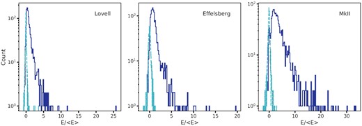
Pulse energy distributions of the single pulses for the Lovell MJDs shown in Fig. 15 and listed in Section 4.3.1, MkII MJDs listed in Section 4.3.1 and Effelsberg MJDs shown in Fig. 9. The on-pulse and off-pulse distributions at each telescope are represented by the solid and dashed lines respectively. Left-hand panel: Single pulses observed at the Lovell telescope at 1564 MHz. Middle panel: Single pulses observed at the Effelsberg telescope at 4 GHz. Right-hand panel: MkII single pulses at 1564 MHz.
4.3.2 Giant pulses
Example GPs from the three telescopes are shown in Fig. 6 and a list of the MJDs corresponding to the GP detections is given in Table A1. The pulse energy distributions of GPs are typically described by a power law (Lundgren et al. 1995a), while the more normal emission can be characterized by lognormal statistics (e.g. Karuppusamy, Stappers & van Straten 2010; Burke-Spolaor et al. 2012). Though the spiky emission reported in Maan et al. (2019) are not GPs by definition, the tails of the distributions of the absolute, and period-averaged peak flux densities are well fit by power laws. The insufficient number of GPs in our Effelsberg and Lovell data do not allow us to fit their distribution. We fit a broken power law to the GPs in the MkII data in Fig. 7. The slope of a power-law fit to the GPs evolves from −1.6 ± 0.1 at the fainter end to −4.8 ± 0.3 at the brighter tail end of the distribution.
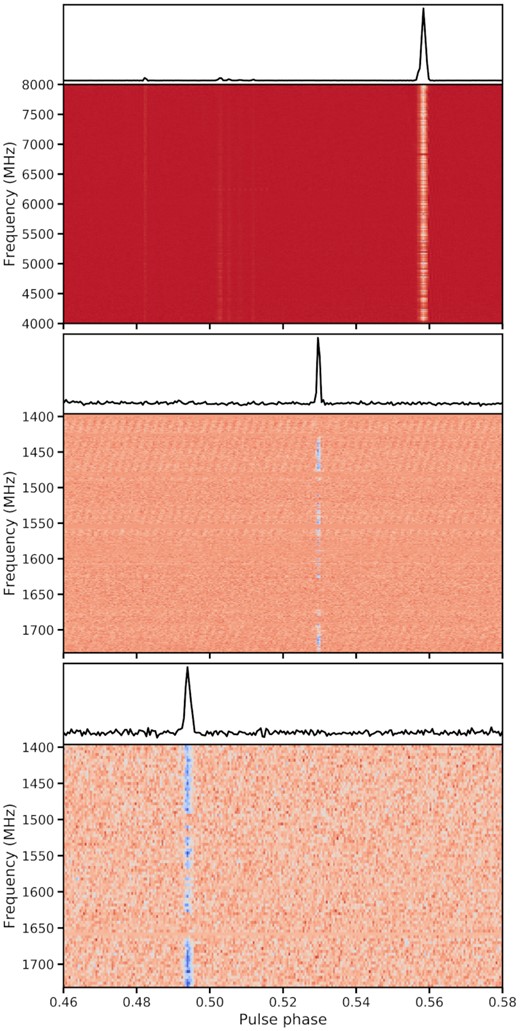
Time-aligned dynamic spectra of example GPs detected with the Effelsberg (top panel; MJD 59009), Lovell (middle panel; MJD 58923), and MkII (bottom panel; left: MJD 59015) radio telescopes. The top panel in each pulse shows the frequency-averaged pulse profile. The data are uncalibrated, and the flux densities are in arbitrary units. The Effelsberg, Lovell and MkII pulses have been decimated to 512, 84, and 84 frequency channels and 2.7 ms resolution, respectively. The background striations seen in the pulse in the middle and bottom panels are due to RFI and not intrinsic to the source. The top panel showcasing the Effelsberg GP also shows barely discernible normal emission between phases 0.48 and 0.52.
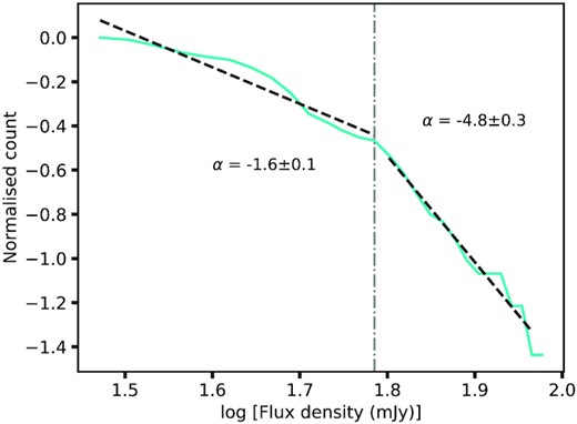
A plot of the cumulative number of GPs detected with the MkII telescope versus their fluxes. The distribution is described by a broken power law with slopes of α = −1.6 ± 0.1 at the fainter end and α = −4.8 ± 0.3 at the brighter tail end.
In addition to their energies exceeding 10〈 E〉 and exhibiting power-law energy distributions, GPs are also characterized by their confinement to narrow pulses phase windows. Fig. 8 shows the distribution of the phases of all the GPs reported in this work. The bi-modal distribution of the MkII data is a result of the two profile components seen in Fig. 9. We observe 61 per cent of the MkII GPs to be confined to the leading pulse phase (ϕ) range 0.473 ≤ ϕ ≤ 0.502 and the remaining 39 per cent to be in the trailing phase range 0.541 ≤ ϕ ≤ 0.567. This preference of the leading over the trailing pulse phase window is similar to what is observed in J0540 − 6919 (Geyer et al. 2021) and contrary to other systems where the GPs lag the normal emission.
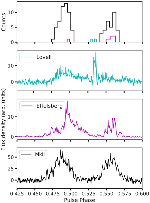
Distribution of phases of the GPs detected at the Lovell, Effelsberg and MkII telescopes. The Lovell and Effelsberg pulse profiles are for MJDs 58923 and 59009, respectively. The MkII profile is the average across all MJDs. Similar to the Crab GPs, the GPs reported here also appear over a narrow range of pulse phases.
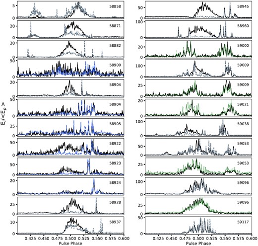
Longitude-resolved distributions of the MkII (dotted, green) and Lovell (dash-dot, blue) telescopes at 1564 MHz, and the Effelsberg (dashed, grey) telescope at 6 GHz. The dash-dot, dotted, and dashed line shows the ratio of the brightest time sample in each pulse-longitude bin, to the average peak flux 〈 Ep〉 at the pulse longitude of the peak of the pulse profile. The solid line is the energy of the average pulse profile scaled to the maximum of the ratio. The profiles have been time-aligned using the best-fitting timing solution and templates (see Section 4.2 for details). Only the data taken with the Effelsberg and MkII telescopes on MJDs 59009 and 59096 are simultaneous.
During the simultaneous observations on 9 June 2020, 13 GPs were detected in the MkII data and 7 GPs were detected in the Effelsberg data. Of the 13 MkII GPs, only 7 occurred during the duration of overlap with Effelsberg observations and all 7 were detected as single pulses in the Effelsberg data. However, only 2 of these 7 simultaneous MKII and Effelsberg pulses were classified as GPs in the both data sets. This is not unexpected, given the large stochastic variations possibly due to a varying spectral index (Lazaridis et al. 2008a; Maan & van Leeuwen 2017; Dai et al. 2019; Pearlman et al. 2020) in the underlying normal emission of the integrated profiles used to calculate the average energies. Fig. 10 shows a comparison of simultaneously detected GPs with the Effelsberg and MkII telescopes. Lazaridis et al. (2008a) present simultaneous and quasi-simultaneous multifrequency observations of XTE J1810 − 197, and show that though the spectrum is generally flat, large fluctuations of the spectral index is observed with time. Simultaneous dual-frequency observations at 8.3 and 31.9 GHz undertaken in Pearlman et al. (2020) show spiky emission. Though Pearlman et al. (2020) do not investigate the existence of GPs, they do note that not all of the emission components were detected at both frequencies suggesting a variable radio spectrum.
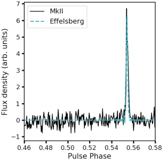
Comparison of a GP detected simultaneously with the MkII and Effelsberg radio telescopes. The data are uncalibrated and the flux densities are in arbitrary units. See Section 4.3 for details.
4.3.3 Longitude-resolved cumulative energy distributions
Another phenomena related to GPs are giant micropulses (Johnston et al. 2001) characterized by extremely large peak flux densities but not so much in terms of their integrated pulse energies. They also have a tendency to be confined to a restricted pulse-longitude range of the overall pulse profile. To investigate this, we produced the longitude-resolved cumulative energy distributions shown in Fig. 9. The brightest time sample in each pulse-longitude bin is compared with the peak flux density of the average profile 〈Ep〉. We see that the highest measured peak flux of a single pulse is ∼150〈Ep〉 at MJD 59009 in the Effelsberg data. We see that GP-like pulses first appeared on MJD 58871, confined to the leading edges of the precursor to the left of the main component of the pulse profile. They then, however, switched positions midway through the observation on 58882 from the left of the main component to its right, and remained on the right of the main pulse until 58945. On 58960, the pulse profile was much spikier than before with GP-like emission at confined phase ranges on either side of the main component, in addition to the leading edge of the main component. Between 59000 and 59117 inclusive, the GP-like emission made an appearance across the entire phase range occupied by the main component, in addition to the component to the right of the main component. As of 59117, the average pulse profile emission was at its spikiest yet, with the fluctuations in the main pulse much more distinct than the other days.
4.4 ACF analysis
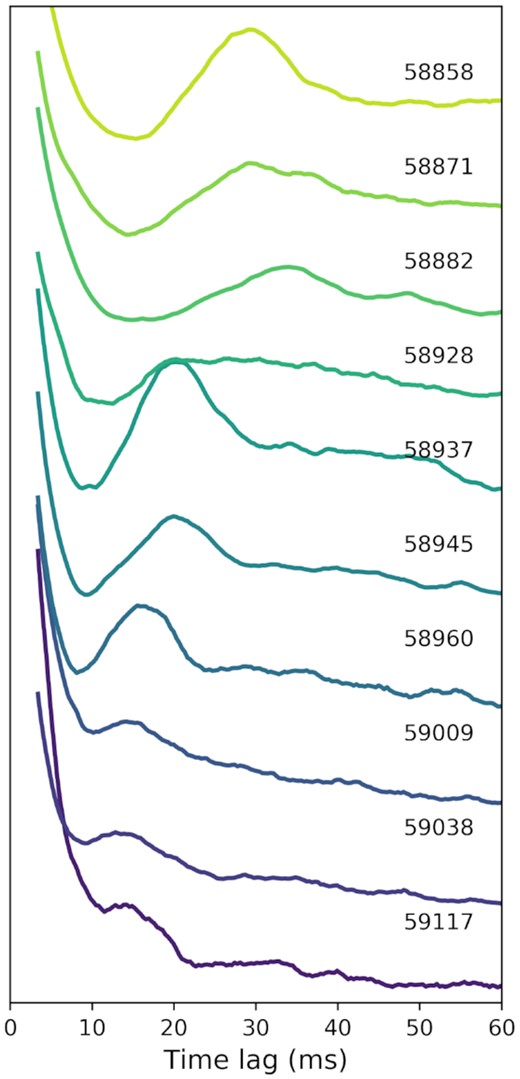
Average ACFs of the Effelsberg data. Individual ACFs of the time-averaged pulse profiles as a function of time lag are shown for each MJD. The time-scale of the characteristic separation between sub-pulses is estimated to be the peak of the first feature following the zero-lag.
5 X-RAY DATA ANALYSIS AND RESULTS
5.1 X-ray light curves
The radio and the X-ray light curves were time-stamped with reference to the Solar System barycentre and the resulting light curve showing overlapping time intervals (see Section 3) is shown in the top panel of Fig. 12. It is visually evident from the plot that there is no obvious correlation between the X-ray and the radio emission. Identifying any underlying correlation between the two wavelengths is more difficult than the previous simultaneous radio and X-ray observations presented in Pearlman et al. (2020) as the X-ray photon counts are at least a factor of 4 lower compared to their data which were closer to the onset of the outburst. Both light curves were folded modulo the topocentric period derived from the best-fitting ephemeris shown in Table 1. The resulting folded X-ray and radio profiles are shown in the bottom panel of Fig. 12. The X-ray profile is best characterized by a simple sine wave with no hint of other components which is dissimilar to the radio profile that shows multiple components within the emission region. It is also important to note that the peak of the X-ray profile is offset from the peak of the leading component of the radio profile by approximately 0.1 in pulse phase which is consistent with the offset seen at the onset of the outburst in 2018 (Gotthelf et al. 2019c). Such an offset between the X-ray and radio pulse is commonly seen in other radio loud magnetars and is expected if the X-ray emission is coming from a different part of the magnetosphere than the open field lines, where the radio emission originates from Gotthelf et al. (2019c).
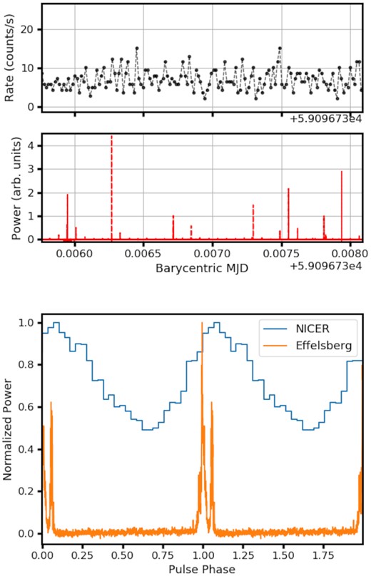
Top Panel: Simultaneous X-ray (NICER, black dots) and radio (Effelsberg, red) barycentred light curves for XTE J1810 − 197 for the observation on 2020 June 09. The lack of correlation with the bright radio pulses is evident, although the counts per bin in the X-ray light curve are not enough for conclusive evidence (see the text for details). Bottom Panel: Folded X-ray (blue) and radio frequency (orange) pulse profile for XTE J1810 − 197 for the same epoch.
5.2 X-ray spectroscopy
In order to study the long-term spectral evolution of XTE J1810 − 197, each observation shown in Table 2 was analysed separately. As the background dominates the spectrum below 0.6 keV and the X-ray flux from the source is extremely weak above 4.5 keV, we only fit the spectra in the 0.6–4.5 keV range. For the spectral fitting, we used the tbabs model in xspec (Arnaud 1996) assuming interstellar medium abundances (Wilms, Allen & McCray 2000). The spectrum was binned so that each spectral channel had at least 25 counts to improve the S/N per spectral channel and facilitate a better fit to the data. Previous spectral studies of XTE J1810 − 197 have shown that a two-component blackbody model and a combination of a power law and a single blackbody component can explain the soft X-ray spectrum (Gotthelf & Halpern 2005). However, the power law is the dominant component in the softer part of the spectrum and there is no physical model that can properly explain or reconcile with the spectrum seen at optical/infra-red wavelengths (Gotthelf & Halpern 2007). Regardless, we decided to fit both (power law + blackbody and blackbody + blackbody) models separately to the spectra to look for the evolution of parameters as a function of time. To search for any statistically significant variations in any of the fitted parameters, we fit for all parameters by keeping only the neutral Hydrogen column density (NH) as a constant. For the purpose of this analysis, we used a NH = 6.5 × 1021 cm−2 (Gotthelf & Halpern 2005). For each observing segment, we fit the spectrum with both the aforementioned models and the resulting best fit parameters are shown in Table 2. We then analysed the evolution of the best-fitting parameters since the onset of the outburst. We clearly see an evolution of our fitted parameters with time and we discuss the implications of this variation in Section 6 (see Fig. 13). We should note that Borghese et al. (2021) used a four blackbody component model to fit the NICER data but the coolest and the hottest components were fixed using the best-fitting values from the XMM–Newton and Nu-STAR data, respectively. Since we only use the nicer data, we decided to fit it with a two blackbody component model. We note that while we have used a similar data set as Borghese et al. (2021), we have analysed the data for a much larger baseline compared to what is presented in Borghese et al. (2021) with an extension of almost another year. We discuss the implications of the results in the next sections.

Left-hand panel: Evolution of the power-law index Γ as a function of MJD. Right-hand panel: Evolution of the blackbody temperatures as a function of time. kTpowerlaw is the single blackbody component that was fit along with the power law. kTcold is the colder blackbody component and kThot is the blackbody component from the hotspot in the polar cap, where we expect the pulsed X-ray emission to originate from.
The 0.5–12 keV spectral parameters for XTE J1810 − 197 for a 2BB model and the PL model. The X-ray flux corresponds to the unabsorbed flux.
| Date | kTwarm | kTcold | Γ | FX, PL (0.5–12 keV) | FX, BB (0.5–12 keV) | Pulsed fraction | Exposure time |
|---|---|---|---|---|---|---|---|
| (MJD) | (keV) | (keV) | (× 10−10 ergs s−1) | (× 10−10 ergs s−1) | (|$\rm {per\,cent}$|) | (s) | |
| 58522.02078704 | 0.75 ± 0.01 | 0.38 ± 0.01 | 1.52 ± 0.04 | 2.450 ± 0.005 | 2.690 ± 0.003 | 28 ± 1.1 | 4826.0 |
| 58571.80939815 | 0.70 ± 0.01 | 0.32 ± 0.01 | 1.74 ± 0.05 | 1.770 ± 0.004 | 1.990 ± 0.005 | 32 ± 1.2 | 4552.0 |
| 58585.67546296 | 0.702 ± 0.01 | 0.32 ± 0.01 | 1.76 ± 0.05 | 1.690 ± 0.003 | 1.860 ± 0.001 | 31 ± 1.5 | 4930.0 |
| 58626.90393519 | 0.71 ± 0.01 | 0.33 ± 0.01 | 1.80 ± 0.05 | 1.470 ± 0.003 | 1.620 ± 0.004 | 35 ± 1.8 | 3529.0 |
| 58702.02623843 | 0.74 ± 0.01 | 0.34 ± 0.01 | 1.77 ± 0.05 | 1.310 ± 0.002 | 1.620 ± 0.004 | 38 ± 1.1 | 3934.0 |
| 58747.18009259 | 0.69 ± 0.01 | 0.30 ± 0.01 | 1.88 ± 0.04 | 1.09 ± 0.03 | 0.954 ± 0.003 | 35 ± 1.5 | 7004.0 |
| 58779.11630787 | 0.67 ± 0.02 | 0.29 ± 0.03 | 2.01 ± 0.20 | 0.851 ± 0.005 | 0.790 ± 0.003 | 33 ± 1.8 | 9290.0 |
| 58943.58254630 | 0.63 ± 0.01 | 0.26 ± 0.01 | 2.33 ± 0.08 | 0.498 ± 0.002 | 0.527 ± 0.001 | 31 ± 2.4 | 4541.0 |
| 59009.14583333 | 0.58 ± 0.01 | 0.27 ± 0.02 | 2.33 ± 0.20 | 0.302 ± 0.002 | 0.336 ± 0.002 | 34 ± 2.2 | 4682.0 |
| 59092.78406250 | 0.64 ± 0.01 | 0.24 ± 0.01 | 2.36 ± 0.07 | 0.262 ± 0.001 | 0.304 ± 0.001 | 30 ± 2.2 | 1684.0 |
5.3 X-ray-pulsed fraction
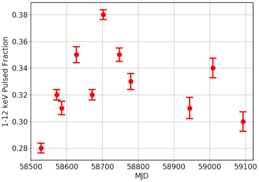
The 1–12 keV pulsed fraction from NICER observations of XTE J1810 − 197 as a function of MJD.
6 DISCUSSION
XTE J1810 − 197 has been regularly monitored and timed with the Lovell, MkII and Effelsberg telescopes from 2009 (Levin et al. 2019) to date, to study the long term evolution of the spin-down rate of the magnetar. Since the middle of 2019 to the beginning of 2020, there has been a steady decrease in the spin-down rate |$|\rm {F1}|$| shown in Fig. 3, reaching a minimum in the beginning of 2020, followed by an increase resulting in a doubling of |$|\rm {F1}|$| since then. Interestingly, this minimum in |$|\rm {F1}|$| corresponds to the onset of the spiky GP-like emission discussed in Section 4.3. The overall amplitude and structure in the evolution of |$|\rm {F1}|$| since the second outburst in 2018 is initially very similar to the one reported in Camilo et al. (2016) and Levin et al. (2019) following the first outburst in 2003. This part of the recovery is also reminiscent of the what has been observed in the spin-frequency recovery of high magnetic field pulsars after an X-ray outburst (Dai et al. 2018). This suggests that high magnetic field pulsars and magnetars plausibly share similar spin-frequency evolutionary traits.
From Fig. 3, we can see that F1 changes significantly over the course of the recovery from the outburst. This is fairly typical of radio-loud magnetars (Kaspi & Beloborodov 2017b), but unlike what is seen in canonical radio pulsars where F1 remains fairly constant or shown variations of much smaller magnitude (see Lower et al. 2020a, and references therein). Hence, one needs to be careful while interpreting inferred quantities like the surface dipole magnetic field strength (B) and the characteristic age (τ) of the magnetar from the measured F0 and F1. The inferred B changes by a factor of 3, while τ changes by a factor of 2 over the time span of our observation thus, demonstrating the issue.
It is unknown at what time after the 2003 outburst the radio pulsations turned on. We note that the time covered by the analysis presented here for data obtained since the 2018 outburst is less than the number of days between the 2003 X-ray outburst and the radio emission turn-off. It is also less than the discovery of pulsed radio emission in the first outburst and the radio emission turn-off. However, we have continued to monitor the source till date, and as of August 2021, it is still visible as a radio emitter after ∼1000 d. It will be interesting to see if the trend in the spin-down evolution from the first outburst is repeated, with the current erratic spin-down behaviour reaching a stable minimum |$|\rm {F1}|$| followed by radio pulsation turn-off within the next ∼1000 d.
The pulse energy distributions of the data from the three telescopes at 1564 MHz and 6 GHz show radio pulses with energies greater than 10〈 E〉, which qualifies them as GPs. This definition of a GP is heavily dependent on the average pulse energy of the underlying emission. In ordinary pulsars, this average pulse energy remains fairly constant over several days. However, we observe a systematic variation in this underlying emission in magnetars, thereby affecting the interpretation of these bright pulses as GPs. While the average pulse energy estimation is based on observations covering MJDs for the Effelsberg data, the average pulse energy per observation was used for the Lovell and MkII data due to the large systematic variations in the underlying emission over a timescale of a few days. We note that for the more recent Lovell data from MJDs 59102, 59103, 59104, 59106, 59118, 59122, 59139, and 59149, we see the appearance of bright normal emission in almost all single pulses in addition to the GP-like emission. While we do not see E/〈 E〉 exceed 10 for any of these pulses, we identify single-peaked pulses from MJD 59104 that have similar flux densities to the GPs seen in earlier Lovell data (see Fig. 15). These pulses are not GPs when defined by comparing their flux to that of the increasing flux density of the underlying emission. However, they are clearly drawn from the same pulse class or type.
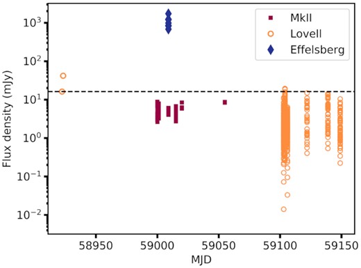
Average fluxes of the GPs detected by the Effelsberg, Lovell and MkII telescopes as a function of MJD. The dashed line marks the flux of a GP at the Lovell telescope whose E/〈 E〉 ∼12. At least two of the pulses from the Lovell data between MJDs 59100 and 59150 represented by open circles are potentially GPs even though they do not meet the criterion in Fig. 5. This is due to the increase in flux of the underlying emission in the recent Lovell data.
The spectra of some magnetars including XTE J1810 − 197 (e.g. Lazaridis et al. 2008b) are known to vary between somewhat positive and negative spectral indices (e.g. Torne et al. 2017). This is reminiscent of FRB pulses (e.g. Spitler et al. 2016; Pastor-Marazuela et al. 2020) as well as Crab GPs (Karuppusamy et al. 2010), which show wildly varying spectra with some pulses brighter at higher frequencies. However, unlike what has been observed in most repeating FRBs, we do not see any evidence of downward frequency drifting with progressing time (Hessels et al. 2019; Caleb et al. 2020). While the number of E > 10〈E〉 GPs detected in the Effelsberg and Lovell data are too low to fit their distribution, a broken power law was found to describe the MkII GPs with a slope of −1.6 ± 0.1 at the fainter end and −4.8 ± 0.3 at the bright end of the distribution. The power-law index of the faint end of the distribution is comparable to those measured for the repeating FRB 20121102A by Gourdji et al. (2019) (−1.8 ± 0.3) and Oostrum et al. (2020) (−1.7 ± 0.6). The power-law index of the bright end of the distribution lies between that of GPs emitted by the Crab at 1.3 GHz (α = −3.36) (Lundgren et al. 1995b) and giant micro-pulses emitted by PSR B1706 − 44 at 1.5 GHz (α = −6.4 ± 0.6) (Cairns 2004).
As there is growing evidence for the association of at least some FRBs being from (young) Magnetars (e.g. Margalit & Metzger 2018), especially because of the exceptionally bright radio pulse seen from the Galactic magnetar SGR 1935 + 2154 CHIME/FRB (Bochenek et al. 2020; Collaboration et al. 2020b) it is worth comparing the brightest of the GPs at all frequencies from XTE J1810 − 197 with those from SGR 1935 + 2154 and the FRBs. In Fig. 16, we compare the specific luminosity of a sample of the GPs seen from XTE J1810 − 197 with a whole range of coherent pulsed radio emitters. We can see that the GPs lie well above the normal pulsars and the majority of the rotating radio transients (RRATs) and are comparable to some of the Crab GPs. They are however still 1–2 orders of magnitude fainter than some of the pulses from the Galactic magnetar SGR 1935 + 2154. We note that the pulse widths used in the estimation of the luminosities of the XTE J1810 − 197 GPs are the observed and not intrinsic widths. As the time resolution is constrained by the sampling time and the scatter broadening seen in both the 6 GHz and 1564 MHz pulses, it means that the GPs could be somewhat narrower and thus move to the left and up in this diagram.
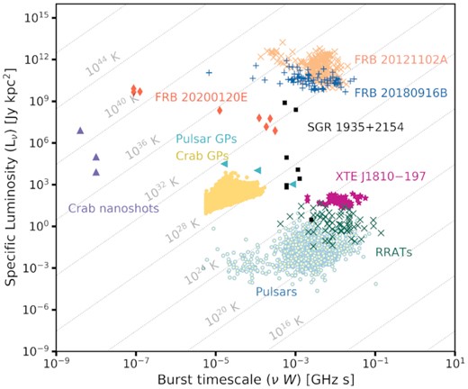
Specific luminosity as a function of burst time-scale of coherent radio sources which emit nanosecond to millisecond duration pulses. The FRBs plotted here are repeating FRBs with well-known distances, and SGR 1935 + 2154 is the radio-loud Galactic magnetar which produced an FRB-like pulse. GPs from XTE J1810 − 197 are seen to sit above the clusters of pulses from rotating radio transients and canonical radio pulsars, forming their own distinct cloud. Figure adapted from Nimmo et al. (2021).
The time-scale of the quasi-periodic modulation is observed to be variable over a time-scale of days (Fig. 11). In the Effelsberg observations on most MJDs, micropulses are visually evident in the single pulse profiles in the form of oscillations superimposed on an envelope, but either do not always feature in the corresponding ACFs or translate into very subtle oscillations. This could be due to either a small number of micropulses in the single pulse ACFs causing them to be washed out in the average ACF, or the absence of any preferred micropulse duration as shown in Cordes et al. (1990). The decrease in the separation between sub-pulses as a function of MJD in the Effelsberg data is consistent with the evolution of the pulse profile in Fig. 9.
During the radio monitoring campaign, the magnetar was also regularly monitored by NICER. This gave us an opportunity to study the spectral evolution of the source since the outburst and if this evolution is in any way related to the radio properties of the magnetar. During the previous outburst in 2003, the X-ray spectrum of the source was well described by a three temperature black-body model with the hottest component proposed to be coming from a small hotspot on the surface and a warmer component coming from another hotspot over a larger surface area and the coldest component coming from the cooling of the entire neutron star surface (Bernardini et al. 2009). It is also possible to explain the spectral evolution of XTE J1810 − 197 with a two component blackbody model without a need of the cool component from the entire surface of the neutron star (Gotthelf & Halpern 2007). Our two component blackbody model fits to the NICER data show that the evolution of the two hot spots on the surface of the neutron star follow a similar trend compared to the previous outburst (Fig. 13). The temperature remains approximately constant for a year before starting to cool down gradually. We also note that the values of the warm and hot component are consistent with the analysis presented in Borghese et al. (2021) with the same data set and are also consistent with those estimated by Gotthelf & Halpern (2007) from XMM–Newton observations of the previous outburst. We also show the evolution of the two blackbody components during the time when GPs were observed. We see the same trend of continued cooling of the hotspot during this time. This time-scale of decay can be explained by the coronal heating model (Beloborodov & Thompson 2007) in which a starquake causes charged particles to be accelerated through a twisted magnetic flux tube while collision of charged particles with the neutron star surface creates the hot spots. While the overall X-ray spectrum is consistent with the previous outburst, the main difference is the complete lack of the 1.1 keV absorption feature that was reported by Bernardini et al. (2009). Typically, absorption features in the X-ray spectra of magnetars can be attributed to proton cyclotron absorption in the magnetosphere that is very much dependent on the magnetic field and the plasma density (Tiengo et al. 2013). To make sure that the absence of this absorption feature was not due a lack of sensitivity, we looked at NICER data close to the outburst where the 0.6–10 keV X-ray flux was a factor of 10 higher than the 0.6–10 keV flux of 5 × 10⁻¹² ergs cm2 s−1 when the 1.1 keV feature was detected during the previous outburst. We do not detect such a feature in any of the NICER data sets. This can be attributed to a couple of reasons. One could be that the XMM–Newton observations were more sensitive to this feature. On the other hand, the feature could be absent due to the different geometry observed during the current outburst. The change in geometry is a likely scenario as many authors have suggested a shift in the magnetosphere of the neutron star due to a starquake if we assume that starquakes cause outbursts in magnetars (Beloborodov & Thompson 2007). While the phase lag between the radio and the X-ray profiles has not changed compared to the previous outburst (Gotthelf et al. 2019a; Borghese et al. 2021), the evolution of flux at radio wavelengths differs significantly compared to the previous outburst, suggesting an evolution in the location of the X-ray/radio emitting regions caused due to a change in the region traversed by the line of sight. This argument is also supported by the evolution of the pulsed fraction observed during the current outburst, which is significantly different from what was observed in the previous outburst (Fig. 14). The value and the evolution of the pulsed fraction depends on the interplay between the line of sight and the location of the hotspot and how the area of the hotspot changes with time. We acknowledge that we cannot rule out the possibility that the different evolution we see in this outburst is caused by the emitting region originating from a different part of the polar cap. Studies of the evolution of the polarization of radio emission from the magnetar will provide a more direct evidence for one of the two possibilities (Desvignes et al. in preparation).
The most recent outburst of XTE J1810 − 197 has been extensively monitored at radio and X-ray wavelengths. While most of these observations are not simultaneous, the span of the monitoring campaigns gives us an opportunity to study the long-term evolution of the X-ray and radio flux of the magnetar since the onset of the outburst. Fig. 17 shows that the evolution is quite different at the two wavelengths. The X-ray flux declines monotonically as expected from the cooling blackbody temperatures that were estimated from the spectral analysis. While the radio flux also initially declines after the outburst, around MJD 58800, the radio flux starts to increase again. The radio flux decreased again before the sudden up turn within a span of three months only to rise again back to the fluxes that were seen at the beginning of this monitoring campaign close to the X-ray outburst. During all this time, the X-ray flux kept decreasing showing no correlation whatsoever with the radio flux. The radio flux density in Fig. 17 seems to roughly track the spin-down rate F1 (or effective magnetic field), which is arguably also large near the start and end of our observations with a minimum near the middle. Such large variations in the radio flux have not been observed in the previous outburst when the radio flux kept decreasing (Camilo et al. 2006). Although, it did show erratic changes in the radio flux for a few weeks before abruptly disappearing as a radio pulsar altogether in 2008 (Camilo et al. 2016).
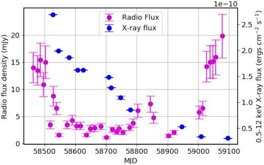
Evolution of radio (1564 MHz) and 0.5–12 keV X-ray flux as a function of time for XTE J1810 − 197 since the onset of the most recent outburst. Note that the X-ray flux has been computed assuming the two blackbody model for the X-ray spectrum (see Table 2).
7 CONCLUSIONS
We report on the detections of GPs, long-term timing properties, and X-ray and radio fluxes during quasi-simultaneous radio and X-ray monitoring of the magnetar XTE J1810 − 197. The GPs made their first appearance on MJD 58922 during observations with the Lovell radio telescope at 1564 GHz and were continued to be seen through to MJD 59054 during observations with the Effelsberg radio telescope at 6 GHz. We report a total of 91 GPs, which satisfy the classic criterion of their flux density exceeding the average flux density by a factor 10 with the Lovell, MKII, and Effelsberg radio telescopes. The onset of the GPs corresponds to a minimum in |F1|. The pulse phases of these GP are confined to narrow ranges, reminiscent of the GP phase windows observed in other sources of GPs. These GPs are comparable in luminosity to the giant radio pulses seen in pulsars, and are one to two orders of magnitude weaker than the lowest energy pulses detected from the Galactic magnetar SGR 1935 + 2154. We continue to see these bright and narrow pulses but by a definition which compares them to the average energy they are no longer strictly GPs. However, we note that this definition fails when all the emission is actually due to GPs, which could be the case sometimes in this source. The systematic variation in the underlying emission of XTE J1810 − 197 between MJDs 59102 and 59149 makes the brightest pulses in that time interval weak compared to the classic criterion of a GP, while they are clearly drawn from the same population of GPs detected at other times. The long-term X-ray evolution of XTE J1810–197 shows that the two blackbody components that best describe the NICER spectrum cool down over time. This is consistent with the previous X-ray outburst shown by this source. At the same time, the 0.5–12 keV X-ray pulsed fraction shows a very different evolution compared to what was seen during the first outburst. While the X-ray flux kept decreasing since the outburst, the radio flux tends to show a slight peak around MJD 58850 followed by a rapid increase in flux that aligns with the onset of GPs. We encourage continued radio and X-ray monitoring of XTE J1810 − 197 in the event of it producing an FRB-like pulse, similar to SGR 1945 + 2154.
ACKNOWLEDGEMENTS
MC, KR, BWS, and MPS acknowledge funding from the European Research Council (ERC) under the European Union’s Horizon 2020 research and innovation programme (grant agreement no. 694745). The authors would like to thank the staff of the Lovell telescope, Effelsberg telescope and the NICER mission for help with the observations. Pulsar research at the Jodrell Bank Centre for Astrophysics and Jodrell Bank Observatory is supported by a consolidated grant from the UK Science and Technology Facilities Council (STFC).
DATA AVAILABILITY
The data underlying this article will be shared on reasonable request to the corresponding author.
Footnotes
REFERENCES
APPENDIX: LIST OF GP DETECTIONS WITH THE EFFELSBERG, LOVELL AND MKII TELESCOPES
GP detections at the Lovell, Effelsberg, and MkII telescopes. The MJDs reported here are within a period of the magnetar.
| Telescope | Topocentric MJDs | S/N | Width (ms) |
|---|---|---|---|
| Lovell | 58922.3907102877 | 361.85 | 8.84 |
| 58923.3009874952 | 580.63 | 11.88 | |
| Effelsberg | 59009.0381518352 | 2965.79 | 9.47 |
| 59009.0387291039 | 1892.83 | 6.08 | |
| 59009.0403326278 | 2961.27 | 7.05 | |
| 59009.0411664603 | 4142.83 | 4.54 | |
| 59009.0448866361 | 2855.32 | 9.51 | |
| 59009.0532249615 | 3094.75 | 5.24 | |
| 59009.0614350054 | 3704.77 | 7.03 | |
| MkII | 59000.0599005787 | 58.71 | 13.77 |
| 59000.0620813383 | 20.95 | 2.34 | |
| 59000.0632999980 | 37.16 | 10.25 | |
| 59000.0638772579 | 19.21 | 1.12 | |
| 59000.0738830964 | 41.32 | 11.88 | |
| 59000.0770900960 | 107.81 | 8.84 | |
| 59000.0792708558 | 93.70 | 10.25 | |
| 59000.0805536557 | 67.76 | 4.90 | |
| 59000.0911367554 | 42.02 | 5.68 | |
| 59000.0954982755 | 86.67 | 7.63 | |
| 59000.0961396755 | 59.39 | 11.88 | |
| 59000.0962038155 | 32.21 | 15.96 | |
| 59000.0981280156 | 37.15 | 11.88 | |
| 59000.1039006160 | 51.58 | 7.63 | |
| 59000.1123029571 | 68.32 | 7.63 | |
| 59000.1149968375 | 33.48 | 6.58 | |
| 59000.1208335787 | 71.03 | 7.63 | |
| 59000.1222446590 | 67.53 | 7.63 | |
| 59000.1267344600 | 73.46 | 10.25 | |
| 59000.1268627401 | 66.17 | 8.84 | |
| 59000.1357140626 | 60.51 | 6.58 | |
| 59000.1378948233 | 65.36 | 24.85 | |
| 59000.1379589633 | 17.06 | 2.34 | |
| 59001.0568292655 | 51.10 | 10.25 | |
| 59001.0627301540 | 35.66 | 4.90 | |
| 59001.0676048012 | 80.90 | 10.25 | |
| 59001.0747884921 | 74.62 | 8.84 | |
| 59001.0779313570 | 51.85 | 10.25 | |
| 59001.0820254615 | 41.06 | 8.84 | |
| 59001.0881937735 | 52.96 | 8.84 | |
| 59001.0895407157 | 94.51 | 10.25 | |
| 59001.0897331360 | 32.97 | 11.88 | |
| 59001.0931967018 | 93.64 | 8.84 | |
| 59001.0933249820 | 45.31 | 10.25 | |
| 59001.0935815425 | 39.02 | 8.84 | |
| 59001.0942229435 | 67.29 | 4.90 | |
| 59001.1021121771 | 45.70 | 8.84 | |
| 59001.1026252980 | 40.24 | 1.29 | |
| 59001.1093600099 | 25.66 | 2.02 | |
| 59001.1097448506 | 109.78 | 4.90 | |
| 59001.1148119197 | 41.30 | 10.25 | |
| 59001.1157098814 | 70.42 | 10.25 | |
| 59001.1158381616 | 57.13 | 10.25 | |
| 59001.1173972215 | 61.93 | 8.84 | |
| 59001.1239198167 | 45.63 | 13.77 | |
| 59001.1251384790 | 28.61 | 11.88 | |
| 59001.1252667592 | 49.64 | 11.88 | |
| 59001.1306545296 | 35.09 | 13.77 | |
| 59001.1355933193 | 58.60 | 7.63 | |
| 59001.1379023638 | 68.37 | 10.25 | |
| 59009.0348197677 | 47.49 | 4.90 | |
| 59009.0361025867 | 52.82 | 10.25 | |
| 59009.0368722781 | 16.63 | 3.64 | |
| 59009.0381550971 | 56.19 | 13.77 | |
| 59009.0387037037 | 90.17 | 5.68 | |
| 59009.0502135961 | 22.73 | 13.77 | |
| 59009.0532282211 | 61.78 | 8.84 | |
| 59009.0702897166 | 57.76 | 5.68 | |
| 59009.0736250468 | 20.62 | 3.14 | |
| 59009.1101854022 | 50.14 | 5.68 | |
| 59009.1180747432 | 43.66 | 11.88 | |
| 59015.0571091614 | 34.57 | 8.84 | |
| 59015.0586485605 | 29.98 | 8.84 | |
| 59015.0730162863 | 63.94 | 8.84 | |
| 59015.0749405355 | 17.94 | 10.25 | |
| 59015.0750046771 | 61.14 | 7.63 | |
| 59015.0780834757 | 52.63 | 5.68 | |
| 59015.0807132829 | 27.53 | 4.22 | |
| 59015.0808415662 | 56.80 | 7.63 | |
| 59015.0846259232 | 52.11 | 4.22 | |
| 59015.0848824896 | 20.13 | 8.84 | |
| 59015.0852031978 | 69.51 | 6.58 | |
| 59015.0862810631 | 39.22 | 8.84 | |
| 59015.0936057531 | 30.75 | 6.58 | |
| 59015.1014310341 | 33.26 | 7.63 | |
| 59020.0113011637 | 49.70 | 7.63 | |
| 59020.0121350120 | 80.24 | 7.63 | |
| 59020.0197679314 | 49.98 | 15.96 | |
| 59020.0218204812 | 54.77 | 11.88 | |
| 59020.0363807573 | 89.90 | 6.58 | |
| 59054.9119285904 | 89.25 | 4.22 | |
| 59054.9295687414 | 126.41 | 6.58 |
