


Abstract
Using a non-local time-dependent statistical theory of convection, we made a linear pulsational instability analysis for stars in the mass range 1.4–3.0 M⊙. The results define a red edge for the δ Scuti instability strip, which fits the observational boundary very well. It is found that the dynamic coupling between convection and oscillation together with the turbulent viscosity are the two main damping mechanisms for low-temperature stars.
1 Introduction
δ Scuti stars are a group of A–F type, short-period variable stars located at the lower extension of the Cepheid instability strip and close to the main sequence. Credit is due to Eggen (1956), who differentiated them from RR Lyrae variables for the first time. The typical pulsational period is shorter than 0.3 d. Most of the variables are pulsating in multiple modes with fairly small amplitudes. Short and multiple periods make them a very important target of astroseismology at the present time. The literal reviews are rich for such types of variables, and include Breger (1979), Eggen (1979) and Wolff (1983).
The non-adiabatic pulsational calculations have been carried out by many authors: among others we recall Chevalier (1971), Cox, King & Tabor (1973), Pamyatnykh (1975), Stellingwerf (1979), Li & Stix (1994) and Breger & Pamyatnykh (1998).
The theoretical blue edge of the δ Scuti instability strip has been well identified so far. However, the red edge has yet never been defined, because of the lack of an exact enough time-dependent theory of convection. Most of the theoretical works did not account for the coupling between convection and oscillation, and it is usual to assume that convection remains constant during the process of pulsation. An exhaustive review was presented by Pamyatnykh (2000) for the existing theoretical approaches to the pulsational instability domain of the δ Scuti variables.
For stars possessing extended convective envelopes, convection takes over radiation and becomes the most important way of energy transport. The stability of these cool stars is controlled by convection through convective energy transfer (the thermodynamic coupling between convection and oscillation) as well as the turbulent pressure and turbulent viscosity (the dynamic coupling between convection and oscillation). In order to treat such couplings, we developed a non-local time-dependent theory of convection (Xiong 1989; Xiong, Cheng & Deng 1997), which is a statistical theory of correlation functions based on hydrodynamics. A better description of the dynamic behaviour of turbulent convection, and a better treatment of the coupling between convection and oscillation can be expected in the framework of such a theory. The present work is the fourth paper in a series dealing with the pulsational stability of stars having extended convective envelopes. The first paper (Xiong, Deng & Cheng 1998, hereafter Paper I) dealt with the oscillations of the luminous red variables. In Paper I, we pointed out that there is a Mira pulsational instability domain apart from the well known Cepheid instability strip. In the second paper (Xiong, Cheng & Deng 1998, hereafter Paper II), we explored the pulsational stability for the horizontal branch (HB) stars. The results of Paper II give rise to a RR Lyrae instability strip which interprets the observations well. The third paper of this series (Xiong, Cheng & Deng 2000, hereafter Paper III) was devoted to solar p-mode oscillations, in which we found out that the coupling between convection and oscillation plays a key role in stabilizing the low-order p-modes  and in exciting the intermediate order p-modes
  All the results are encouraging for our theory. The present work is for the oscillations of δ Scuti stars, and the main goal is to explore the red edge of the instability strip. In Section 2, we describe briefly the equilibrium model and the key points of pulsation computation. The results of non-adiabatic oscillations are given in Section 3. In Section 4, we present a theoretical insight of the coupling between convection and oscillation, and an interpretation for the red edge of the δ Scuti instability domain. A brief summary and the discussion is given in Section 5.
2 The equilibrium models
11 stellar evolutionary tracks have been calculated for stellar mass range  using the Padova stellar evolutionary code described by Bressan et al. (1993). All evolutionary models have the solar composition
 , and an intermediate overshoot of 0.25 Hp above the convective core is considered. 30–40 envelope models have been calculated for each of the tracks, and this gives rise to a total of 415 envelope models. An analytic approach of opacity to the OPAL (Rogers & Iglesias 1992) and the low-temperature opacity tables (Alexander & Ferguson, 1994) is used in the numerical calculations of equilibrium models and oscillations. Such a treatment makes it very convenient to obtain opacities for different compositions and very smooth interpolation; it also gives more precise derivatives of opacity against temperature and pressure, χT and χp, for pulsation calculations. A modified MHD equation of state is applied throughout the calculations of the equilibrium models and oscillations. All the original theoretical considerations of the MHD equation of state (Dappen et al. 1988; Hummer & Mihalas 1988; Mihalas, Dappen & Hummer 1988) are included. A main simplification is to assume that the helium atom is considered as a quasi-hydrogen atom. For the highly excited states, a neutral helium atom behaves in a very similar way to a hydrogen atom. The sizable deviation happens only for the fundamental state of neutral helium. Such an approximation significantly simplifies the calculations of the equation of state, without adding any large errors to the equation of state and the thermodynamic quantities. So, instead of using interpolations of the pre-compiled tables of the equation of state and thermodynamic quantities, we can take the calculations for them in real time, constructing the equilibrium models and getting the thermodynamic quantities of gas needed in the pulsation calculations. The equation of state applied here includes: the decomposition of molecular hydrogen; the neutral, first and second ionizations of helium; the neutral and ionized states for hydrogen and eight metals with low ionization potentials, and the Debye–Huckel Coulomb correction. The radiative pressure as well as the excitation energy of atoms and the energy of radiative field are all considered in calculation of state parameters. We believe that our treatment of the opacity and the equation of state makes our results from the pulsation calculations more accurate.
The coupling between convection and oscillation was taken into account in the pulsation calculations. Convection is handled by using a non-local time-dependent theory (Xiong 1989; Xiong, Cheng & Deng 1997). The stellar structure equations and the dynamic equations of turbulent convection compose a set of self-consistent radiative-hydrodynamic equations (Xiong 1989). When the terms of time-derivatives are ignored, we get the set of equations for equilibrium models. Linearization of the radiative-hydrodynamic equations gives rise to a set of 10 equations for linear non-adiabatic oscillations, six of which are used to describe the dynamic behaviour of convective motions. When we further put all the convective Lagrangian variations to zero, the number of equations is reduced to four. Then convection and oscillation are decoupled in this case. The pulsation equations and boundary conditions are the same as in Paper I. For pulsation calculations, the outer boundary is put at a thin enough optical depth:  the lower boundary is also deep enough, with the temperature being
  The stellar core region has almost no effects on the pulsational stability. The number of grids used in this work is 800.
3 The pulsational instability strip
Following the method outlined in the above section, we calculated linear non-adiabatic oscillations for the first 12 modes of 415 stellar models along the 11 evolutionary tracks with masses  Fig. 1(a) displays all the unstable models (at least one mode is unstable) on the Hertzsprung–Russell (HR) diagram. The dashed lines labelled ‘BE’ in Figs 1 and 2 are Pamyatnykh's (2000) theoretical blue edge of the δ Scuti instability domain for radial pulsations, which is defined by the hottest pulsationally unstable models. The black line labelled ‘RE’ is the emprical red edge of the δ Scuti instability strip, estimated using observational data (Pamyatnykh 2000). It is clear from Fig. 1(a) that our theoretical red edge of the instability domain matches the observational one very well, except at the lower part where our results are slightly redder than the observations. As is also shown by Fig. 1(a), our blue edge fits Pamyatnykh's blue edge pretty well, with a little difference close to the zero age main sequence (ZAMS), where our models are redder than Pamyatnykh's by
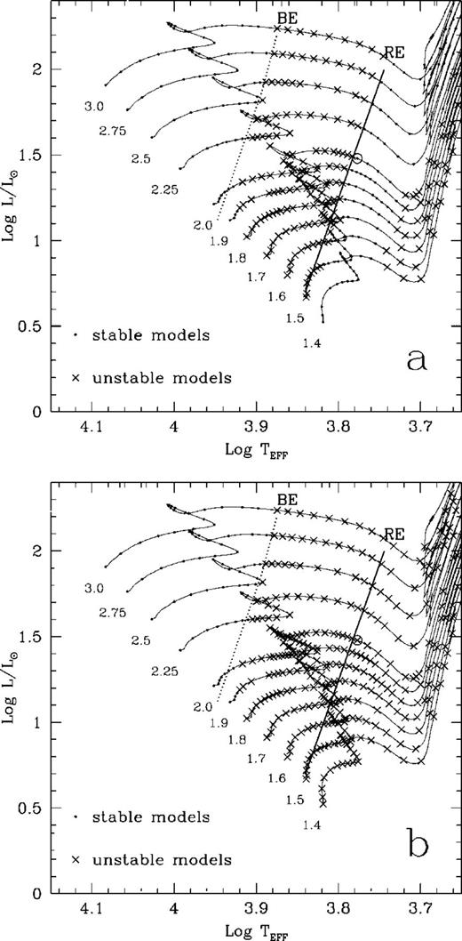
The location of the pulsationally unstable modes denoted by crosses (there is at least one unstable mode from the fundamental to eighth overtone) and the stable modes denoted by small dots in the HR diagram. In panel (a) the coupling between convection and oscillation is included; in panel (b) the coupling is ignored.
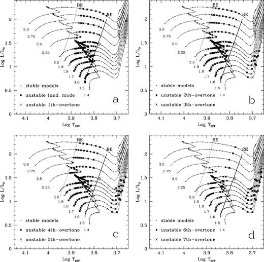
The distribution of the unstable modes in the HR diagram. (a) The pulsationally unstable fundamental (large solid dots) and the first overtone (crosses); (b) the second and third overtones (large solid dots and crosses, respectively); (c) the fourth and fifth overtones (large solid dots and crosses, respectively); (d) the sixth and seventh overtones (large solid dots and crosses, respectively). The small dots are pulsationally stable models.
Figs 2(a)–(d) display the locations of the unstable models from the fundamental mode to the seventh overtone on the HR diagram respectively. It is clear from Fig. 2 that our theoretical unstable strip reaches the bluest point for the third to the fifth overtone. Towards higher overtones, the unstable strips narrow very quickly. In Pamyatnykh's blue edge, the upper part is defined by the hottest unstable third and fourth overtone models (the same as ours), while the lower part is given by the unstable high order overtones (sixth and seventh modes). We have not yet clarified the cause of the difference between Pamyatnykh's results and ours. We think it may be because of the surface boundary conditions used in the calculations. For the fundamental and lower order overtones, the surface boundary conditions and the altitude located are not critical. In going towards higher-order overtones, the effects of the outer atmosphere on stellar oscillations grow quickly. For our case, the surface boundary condition is put at a very shallow optical depth  We have also computed the linear non-adiabatic oscillations with the same pulsational code, but the surface boundary was located at optical depths
  and 0.66 respectively. Unno's surface mechanical and thermal boundary conditions at infinite optical depth were used (Unno 1965). The result of
  is very close to that of
  However, the result of
  is markedly different from the formers. A careful inspection of figs 3 and 4 of Pamyatnykh's (2000) paper shows that the blue edge of the lower part of the instability domain seems to be so hot as to be incompatible with observations. It might be possible that the hot dwarfs near the ZAMS are pulsating at such small amplitudes that they cannot be detected by observations. It is still uncertain whether Pamyatnykh's blue edge or ours is correct. We have to wait for further observational evidence.
A rather interesting theoretical result was found from our calculation. As shown in Fig. 1a, the coolest stars in the red giant branch (RGB), far away from the δ Scuti instability strip, are pulsationally unstable. It is even clearer from Figs 2(a)–(d) that the fundamental and the first overtone of these red stars are pulsationally stable. However, the second- and high-order overtones are unstable. Blanco & Plaut (1965) had reported that the light variations are a common observational fact for red giants with spectral types later than M4. But the amplitudes are rather small (<0.5 mag) up to M7, from which they become larger for later types. Yao (1981, 1986, 1987) found some short-period low-amplitude variables in the RGB of globular clusters. Although it is still a problem and a dispute, we believe that the RGB stars are possibly pulsating at certain amplitudes. This is beyond the scope of the present work, and we will not go into details of this problem here.
4 The red edge of the δ Scuti instability strip
The blue edge of the δ Scuti instability strip has been studied heavily in literature, so we are not going to say more than is necessary. In this section we will concentrate on the red edge. It is certain that the existence of the red edge is caused by convection. It is impossible to interpret the red edge if the coupling between convection and oscillation is not considered. Fig. 1(b) displays the distribution of the unstable modes when the coupling between convection and oscillation is ignored (i.e. assuming that convection is constant during the process of pulsation). It can be seen from Fig. 1(b) that all the models on the right-hand side of the blue edge of the instability strip are pulsationally unstable, so no red edge can be given in this case.
For the hot stars close to the blue edge, the surface convective regions are not significant. Therefore convection does not seriously affect oscillation, and the excitation in that case is mainly caused by the κ mechanism. Moving to the middle of the instability strip, the zone of partial ionization of hydrogen becomes convective. Convection has important effects on the instability of the high-order overtones. The fundamental and low-order overtones are excited by the deeper second ionization of helium, therefore convection does not seriously affect these modes. For the low-temperature stars close to the red edge, however, even the second ionization helium zone becomes convective. Convection in these red stars takes over radiation and becomes the dominant mechanism controlling the pulsational instability.
The pulsational instability of cool stars with extended convective envelopes is controlled by convection through convective energy transfer (the thermodynamic coupling), and turbulent pressure and viscosity (the dynamic coupling). In a previous work (Paper III) we have explained in detail how these mechanisms affect the solar p-mode oscillations. The main conclusions can be summarized as follows:
- (i)
Turbulent viscosity is always a damping mechanism for oscillations, because it converts the orderly kinetic energy of pulsaton into chaotic kinetic energy of turbulence and eventually into thermal energy.
- (ii)
Turbulent pressure generally works as excitation, at least in the regions where the non-adiabatic effects are not serious. The reason is that the variations of turbulent pressure always lag slightly behind those of density during the process of stellar pulsations. On the P–V power diagram, it performs a clockwise Carnot cycle, i.e. the turbulent kinetic energy is converted into orderly pulsational kinetic energy.
- (iii)
The turbulent thermal convection (the thermodynamical coupling) is always a damping factor in the deep layers inside the convective zones. Generally speaking, when stars are in the contraction phase, the convective energy transfer intensifies, while in the expanding phase convective energy transfer weakens, and in the stellar interior the relative amplitude of convective flux
 where L is the total luminosity) grows outwards. The combination of these two effects makes the fluid elements lose their thermal energy through convective energy transfer in the contraction phase of relatively high temperatures and get thermal energy in the expanding phase of relatively low temperatures during the process of pulsation. This is something like a refrigeratory: losing energy at a higher temperature while gaining energy at a lower temperature. It performs a counterclockwise Carnot cycle on the P–V power diagram, and converts pulsational kinetic energy into thermal energy. Near the top of the convective zone, the relative amplitude of the convective flux
  and the convective energy flux Lrmc decrease towards surface of star. Therefore, the relative amplitude of the convective flux
  also decreases outwards. This enables fluid elements to get energy in the contraction phase of relatively high temperature and to lose thermal energy in the expanding phase of relatively low temperature during the process of pulsation. Therefore convective energy transfer (the thermodynamical coupling) is a pulsational excitation mechanism over there. An increase of the pressure component of work, Wp, towards the surface (in Figs 3a–d) results mainly from this excitation effect of thermodynamical coupling. A more detailed argument for the effect of thermodynamical coupling on the excitation and damping of stellar oscillations can be found in section 2.1 of Paper I and section 4 of Paper III.
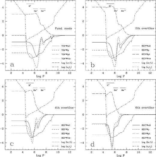
The variations of the total integrated work Wall (solid curve) and its gas pressure component Wp (dashed line), the turbulent pressure component Wpt (long dashed line) and the viscosity component Wvis with depth in log P. The normalized radiative flux  and ωrτc are also plotted and labelled, where ωr is the pulsational cyclic frequency, and τc is the local inertial time-scale for convection. The panels show (a) the fundamental mode; (b) the second overtone; (c) the fourth overtone; (d) the sixth overtone. The parameters of the stellar model are
 and
and  This model is just located outside the red edge of the instability strip. This model is labelled with circles in Figs 1 and 2.
The three basic arguments above hold for all stars with extended convective envelopes. The ultra-luminous stars that show extreme non-adiabatic properties are slightly complex. Due to such extreme non-adiabatic nature, the simple phase relations mentioned above are lost. The curves of Wp and Wpt will become complex as a result of the strong coupling between the gas pressure and turbulent pressure. For example, it happens in the long period variables discussed in Paper I. Nevertheless, the comments on the effects of the dynamical and thermodynamical couplings on the pulsational stability of stars mentioned above still hold, especially for such stars as the low-luminosity δ Scuti stars and RR Lyrae.
Figs 3(a)–(d) display the normalized integrated works of the fundamental, second, fourth and sixth overtones against depth, for a star just outside the instability strip (labelled by an open circle in Figs 1 and 2). In order to show all the effects caused by turbulent convection, not just the total integrated work,  but also the gas and radiative pressure
  component Wp, the turbulent pressure component Wpt and the viscosity component Wvis are given in Fig. 3. Also plotted in Fig. 3 is the variation of the normalized convective flux
  versus depth. In Figs 3(a)–(d), the three horizontal bars indicate the partial ionization region of hydrogen, and the first and second ionization regions of helium, respectively (the regions are bound by the ionization degree
The normalized integrated work is defined here by the increase rate of pulsational kinetic energy per period, divided by the total pulsational kinetic energy. The derivation is trivial and can be outlined as follows: multiplying the fluid dynamic equations by the conjugate component of velocity and the mass of the element, then integrating from the stellar centre (actually from the bottom of the static envelope model) to surface, we can get the integrated work Wall and its components, Wp, Wpt and Wvis. Their expressions are referred to in Paper III. According to the definition of the normalized integrated work, we can know that its value at the surface should be equal to the growth rate of pulsational amplitude  where ωi and ωr are respectively the imaginary and real parts of the complex frequency:
  is obtained from non-adiabatic pulsation. Our numerical results show that Wall matches η very well; the deviation is generally within 2 per cent and the maximum is 4 per cent. This makes us confident about our results.
By the definition of the integrated work, it is easy to understand that when the work curve grows outwards, the region is an excitation zone. Otherwise, it is a damping zone. Figs 3(a)–(d) have firmly verified the three arguments given at the beginning of this section. They can be strengthened and concluded as the follows:
- (i)
The turbulent viscosity is a real damping mechanism, which is more important for the high order overtones. This is due to the fact that the turbulent viscosity component of total work is proportional to the square of velocity gradient, i.e.
 For higher-order overtones, the relative amplitude of pulsation decreases even faster towards the stellar centre.
 - (ii)
Wpt normally grows outwards. This means that the turbulent pressure is indeed an excitation mechanism.
- (iii)
In the deep interior of convective zone the gas and radiative pressure component of the integrated work, Wp, generally decreases outwards. Therefore, this is a damping region. The pressure component, Wp, contains the contribution of both convective energy transfer (the thermodynamical coupling) and radiative energy transfer, and it is hard to separate them. In fact, in the convection zone the radiative flux Lr is far less than the convective flux Lc. Except the two gradient regions of radiative flux at the top and the bottom of the convective zone and the regions where the temperature derivative of opacity χT varies violently, the contribution of convective flux generally dominates. The Wp curve basically expresses the contribution of the thermodynamic coupling between convection and oscillation. We can note that two localized bumps on the Wp curve in Fig. 3(a), which corresponds to the contributions of the κ mechanism caused by the ion and helium absorption bumps.
Following Figs 3(a)–(d), we found that the excitation and damping regions of pulsation are shifting to outer layers as the pulsational mode increases from the fundamental to higher-order overtones. The bumps on the Wall and Wp curves also shift to a shallower depth, and they eventually disappear. This is caused by the faster decreases of the relative pulsational amplitudes inwards for the high-order overtones.
As shown by the above analysis, we can see that the thermodynamical coupling between convection and oscillation and the turbulent viscosity are the key factors for determination of the red edge of the δ Scuti instability strip.
5 Conclusions and discussions
Using a non-local time-dependent theory of convection (Xiong 1989; Xiong, Cheng & Deng 1997), we have computed the linear non-adiabatic oscillations for several types of pulsating stars. In the first work of this series, we calculated non-adiabatic oscillations for the luminous pulsating red variables. Normally, convection was thought of as a damping factor for stellar pulsations. Our results show that it cannot be treated as if it is lumped together. The turbulent viscosity is the only pure damping factor. Wvis is proportional to  where ω is the cyclic frequency of pulsation, τc is the inertial time scale of convective motion. In the convection zone of luminous giants and super-giants
  for the fundamental mode. Therefore turbulent viscosity has little damping effects for oscillations of the fundamental and first modes of these luminous red stars. While for dwarfs and less luminous giants,
  mostly in the domain of the convection zone. The turbulent viscosity becomes an important damping factor against pulsation. Generally speaking, turbulent pressure is an excitation mechanism for stellar pulsation. The effect of convective energy transfer (the thermodynamic coupling), however, is different in the different positions of the convection zone. It is damping in the deep interior, while excitation is on the top of the convective zones. Therefore, thermodynamic coupling is the main damping factor for oscillations of the fundamental and low-order modes of cool stars. However, it may become an excitation mechanism for high-order modes. The relative sizes of Wp, Wpt and Wvis vary with the mass, luminosity, effective temperature and pulsational mode of the star. Each component of integrated work may have different contribution to the pulsational stability, depending on these basic stellar parameters and pulsational mode. Such a complicated interaction between convection and oscillation provides a natural explanation for the existence of red edges of the δ Scuti instability strip (this work) and the RR Lyrae instability strip (Paper II). It also leads to an understanding of the mystery of the Mira instability domain outside the Cepheid instability strip (Paper I). Furthermore, the high-luminosity red variables are pulsating at the fundamental and low-order overtones, and all the high-order overtones of them are pulsationally stable. On the contrary, the intermediate- and low-luminosity red giants are stable in the fundamental and low-order modes, but they are pulsating at high
  modes (Paper II and this work). For the dwarf stars such as the Sun, the unstable modes are still higher overtone modes
  Starting from the same theory, we can interpret several typical types of pulsating variables. This is a direct proof that our convection theory is basically correct.
A quantitative comparison between the theoretical results and observations tells us that our results are the best for dwarf stars such as the Sun and δ Scuti stars (we should say that the regular coupling between convection and oscillation cannot completely explain the excitation of the solar p modes, as this is claimed in Paper III. Apart from the regular coupling between convection and oscillation, there must be some other excitation and damping mechanisms, and we think that the turbulent stochastic excitation is the best candidate). For RR Lyrae stars, a fairly good match between theoretical results and observations has been realized (Paper II), but our theoretical red edge is already redder than Sandage's observed one (Sandage 1990) by  For even more luminous red variables, we can merely point out that there exists a Mira instability domain. However, we cannot delimit its precise boundary on the HR diagram. By a careful insight of the difference between the structure of the convective regions of dwarf and giant stars, we found that the convective motion is subsonic for dwarfs, while it becomes strongly supersonic on the top of the convective region for giants and supergiants because of the very low efficiency of convective energy transfer, which makes the convection there strongly super-adiabatic. In the super-adiabatic region, although convection contributes little to energy transfer, the properties of such super-adiabatic convection are extremely important for the structure of the whole convective region. The size of the convective region is actually determined by the structure of the super-adiabatic region (Xiong & Cheng 1992). The existing theory of convection can only be applied to subsonic convection, and we have taken this as a basic assumption, i.e.
  and
and  (Xiong 1989; Xiong, Cheng & Deng 1997). The mixing length theory (MLT) is not a hydrodynamic theory, but a ‘ballistic’ theory. Actually, the assumption of subsonic convection is also implicated in the MLT. Sound speed is actually a critical point in hydrodynamics. The supersonic convection has completely different property from the subsonic convection. Therefore, applying a theory for subsonic convection directly to supersonic case without any modification will certainly cause errors. It is, we think, an evidence of supersonic convection that our theory gives good results for dwarf and sub-giant stars, and going to high luminosity, the theoretical results become worse. We feel a strong need to develop a theory of convection, which is applicable to both domains of subsonic and supersonic convection. Undoubtedly, it is an extremely difficult subject.
References
