


Abstract
For a perfectly calibrated forensic evaluation system, the likelihood ratio of the likelihood ratio is the likelihood ratio. Conversion of uncalibrated log-likelihood ratios (scores) to calibrated log-likelihood ratios is often performed using logistic regression. The results, however, may be far from perfectly calibrated. We propose and demonstrate a new calibration method, “bi-Gaussianized calibration,” that warps scores toward perfectly calibrated log-likelihood-ratio distributions. Using both synthetic and real data, we demonstrate that bi-Gaussianized calibration leads to better calibration than does logistic regression, that it is robust to score distributions that violate the assumption of two Gaussians with the same variance, and that it is competitive with logistic-regression calibration in terms of performance measured using log-likelihood-ratio cost (Cllr). We also demonstrate advantages of bi-Gaussianized calibration over calibration using pool-adjacent violators (PAV). Based on bi-Gaussianized calibration, we also propose a graphical representation that may help explain the meaning of likelihood ratios to triers of fact.
1. Introduction
A set of scales should be well calibrated, otherwise its readout will be misleading. If a set of scales is well calibrated, when an item is placed on the set of scales, the value of its readout will equal the mass of that item. Figure 1 shows, for a perfectly calibrated set of scales, the relationship between the mass placed on the set of scales and the readout of the set of scales—this is the identity function, we will also refer to it as the “perfect-calibration line.” The process of calibrating the set of scales involves adjusting its calibration settings so that its readouts over a range of masses are as close as possible to the identity function.
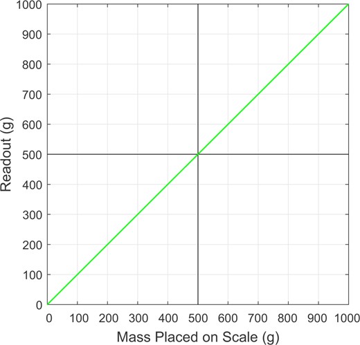
The relationship, for a perfectly calibrated set of scales, between the mass placed on a set of scales and the readout of the set of scales—this is the identity function/the perfect-calibration line.
The following is a perfectly calibrated system: a system for which the distribution of the natural logarithms of the likelihood ratios that it outputs in response to different-source input pairs and the distribution of the natural logarithms of the likelihood ratios that it outputs in response to same-source input pairs are both Gaussian and both have the same variance, and , and the means of the different-source and same-source distributions are and , respectively (Peterson et al. 1954: Sections 4.3 and 4.9; Birdsall 1973: Section 1.3; Good 1985: Section 6; van Leeuwen and Brümmer 2013; Morrison 2021).1
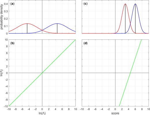
(a) Different-source and same-source Gaussian distributions with, , , . (b) Log-likelihood-ratio-to-log-likelihood-ratio mapping function corresponding to (a). (c) Different-source and same-source Gaussian distributions with, , , . (d) Score-to-log-likelihood-ratio mapping function corresponding to (c). Panels (a) and (b) represent a perfectly-calibrated system. Panel (b) shows the identity function.
The identity function can be obtained by applying the procedure described above to any perfectly calibrated bi-Gaussian system, irrespective of the value of . The panels in the left column of Fig. 3 show examples of different-source and same-source distributions of perfectly calibrated bi-Gaussian systems with different values of . All panels represent perfectly calibrated systems, but the performance of systems represented in lower panels is better than the performance of systems represented in higher panels—the overlap between the different-source distribution and the same-source distribution is less. From the top panel to the bottom panel, the corresponding log-likelihood-ratio cost () values are 0.85, 0.52, 0.24, and 0.09. The panels in the right column of Fig. 3 show the Tippett plots corresponding to the panels in the left column.2
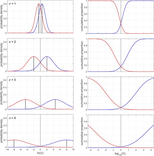
Left column: different-source and same-source distributions of perfectly calibrated bi-Gaussian systems with different values of . Right column: Tippett plots corresponding to the distributions in the left column. From the top to the bottom panel, the corresponding values are 0.85, 0.52, 0.24, and 0.09.
The mapping function in the example in Fig. 2d has slope and intercept . If this mapping function is applied to the distributions in Fig. 2c, the result is Fig. 2a. If the same procedure is then applied to the already-calibrated distributions in Fig. 2a, the mapping function in Fig. 2b has slope and intercept , that is, it is the identity function.
In the example above, the different-source score distribution and the same-source score distribution were both Gaussian and they had the same variance. In these circumstances, the calibration model can be based on an LDF as described in Equation (4). In practice, the assumption that the score distributions consist of two Gaussians with the same variance is often violated. Therefore, rather than using an LDF, the intercept and slope, and , are usually obtained using logistic regression (LogReg), which is more robust to violations of this assumption (Brümmer and du Preez 2006; González-Rodríguez et al. 2007; Morrison 2013; Morrison et al. 2020, 2023). Notice, however, that since the calibration function is still a linear mapping in the space, if the score distributions violate the assumption of two Gaussians with the same variance, then the “calibrated” distributions will not consist of two Gaussians with the same variance, and hence may be far from the same-source and different-source distributions of a perfectly calibrated bi-Gaussian system. The pool-adjacent violators (PAVs) algorithm (Ayer et al. 1955; Zadrozny and Elkan 2002; Brümmer and du Preez 2006), aka isotonic regression, has been used to provide a non-linear but monotonic mapping, but this non-parametric approach overfits on the training data and therefore does not generalize well to new data. Also, it does not extrapolate below the lowest same-source value and above the highest different-source value.4 Using kernel-density estimates (KDEs) of the same-source scores and of the different-source scores, dividing the former by the latter, and taking the logarithm results in a non-linear mapping, but one which is not monotonic. Conversion of uncalibrated likelihood ratios to calibrated likelihood ratios, and indeed calibration in general, should be monotonic.
This article proposes and demonstrates the use of a new calibration method, “bi-Gaussianized calibration,” that uses a non-linear monotonic function to map scores toward a perfectly calibrated bi-Gaussian system.
The remainder of this article is organized as follows:
Section 2 describes the bi-Gaussianized calibration method.
Section 3 demonstrates the application of the method on two sets of simulated data and on two sets of real data.
Section 4 explores the effect of sampling variability on the performance of the method.
Section 5 describes a graphical representation that may facilitate understanding by the trier of fact of likelihood-ratio values output by the method.
Section 6 provides a conclusion.
The data and Matlab® code used for this article are available from https://forensic-data-science.net/calibration-and-validation/#biGauss. This includes a function that implements bi-Gaussianized calibration and a function that draws the graphical representation described in Section 5. Python versions of the latter functions will also be made available.
2. Bi-Gaussianized calibration method
2.1 Variants
Below, we describe four variants of bi-Gaussianized calibration. Each variant uses a different method to calculate the for a target perfectly calibrated bi-Gaussian system. Three variants include an initial calibration step using LogReg, KDE, or PAV, then calculate the target based on , and the other variant calculates the target based on equal-error rate (which we will abbreviate as or EER depending on context). Scores are then mapped toward the of the perfectly calibrated bi-Gaussian system with the target .
In the remainder of this section:
We describe the steps required to implement each variant of the bi-Gaussianized-calibration method.
We derive, for a perfectly calibrated bi-Gaussian system, the relationship between and , and the relationship between and .
We compare the performance of the EER, LogReg, KDE, and PAV methods for determining the target .
We describe the algorithm for mapping from the cumulative score distribution to the cumulative distribution of the perfectly calibrated bi-Gaussian system with the target .
2.2 Steps for the -based variants
The -based variants of the bi-Gaussianized-calibration method consist of the following steps:
Calculate same-source scores and different-source scores (uncalibrated log-likelihood ratios) for a set of training data and a set of test data.
Calibrate the training-data output of Step 1 using one of the following methods: LogReg5; KDE6; PAV.7
Calculate for the output of Step 2.
Determine the of the perfectly calibrated system with the same as calculated at Step 3.
Ignoring the same-source and different-source labels, determine the mapping function from the empirical cumulative distribution of the training-data output of Step 1 to the cumulative distribution of the perfectly calibrated bi-Gaussian system (a two-Gaussian mixture) with the determined at Step 4.
Apply the mapping function determined at Step 5 to the test-data output of Step 1, and to the score calculated for the comparison of the actual questioned- and known-source items in the case.
2.3 Relationship between and
Although, in general, there is a many-to-one mapping in which different sets of same-source and different-source likelihood ratios can map to the same value, there is a one-to-one mapping between the of a perfectly calibrated system and the of that system. Step 4 requires that the latter mapping be known. Given , if one can determine , then one knows everything about the same-source and different-source distributions of that perfectly calibrated system.
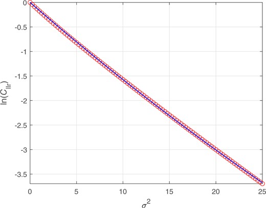
Circles: values given values. values were calculated using numerical integration applied to Equation (6). Curve: Fitted regression of on .
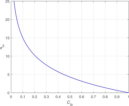
Relationship between and for a perfectly calibrated bi-Gaussian system.
This subsection has derived the relationship between and for a perfectly calibrated bi-Gaussian system. Instead of using , any other strictly proper scoring rule (SPSR) could be used. One would have to derive the relationship between that SPSR and for a perfectly calibrated bi-Gaussian system. We use , rather than any other SPSR, because it is commonly used in the forensic-science literature.
2.4 Steps for the -based variant
The -based variant of the bi-Gaussianized-calibration method consists of the steps listed below. Steps 1, 5, and 6 are identical to the -based variants, and Steps 3 and 4 are parallel. The -based variant has no parallel of the -based variants’ Step 2.
Calculate same-source scores and different-source scores (uncalibrated log-likelihood ratios) for a set of training data and a set of test data.
Skip.
Calculate the for the training-data output of Step 1.
Determine the of the perfectly-calibrated system with the same as calculated at Step 3.
Ignoring the same-source and different-source labels, determine the mapping function from the empirical cumulative distribution of the training-data output of Step 1 to the cumulative distribution of the perfectly calibrated bi-Gaussian system (a two-Gaussian mixture) with the determined at Step 4.
Apply the mapping function determined at Step 5 to the test-data output of Step 1, and to the score calculated for the comparison of the actual questioned- and known-source items in the case.
2.5 Relationship between and
is the value at which the false-alarm rate (FAR) and miss rate (MR) are equal. To calculate we used an algorithm that sorted the data from Step 1 irrespective of different-source or same-source label, calculated FAR and MR at each datapoint (FAR monotonically decreases and MR monotonically increases), found the first datapoint for which FAR was less than MR, then took the mean of FAR and MR at that datapoint or the mean of FAR and MR at the immediately preceding datapoint, whichever was lower.12 If FAR was zero, the mean was calculated using the MR obtained as described above and half the lowest non-zero FAR. If MR was zero, the mean was calculated using the FAR obtained as described above and half the lowest non-zero MR. If FAR was never less than MR, the mean was calculated using half the lowest non-zero FAR and half the lowest non-zero MR.
Although, in general, there is a many-to-one mapping in which different sets of same-source and different-source likelihood ratios can map to the same value, there is a one-to-one mapping between the of a perfectly calibrated system and the of that system. Step 4 requires that the latter mapping be known. Given , if one can determine , then one knows everything about the same-source and different-source distributions of that perfectly calibrated system.
Figure 6 shows the relationship between and for a perfectly calibrated system.
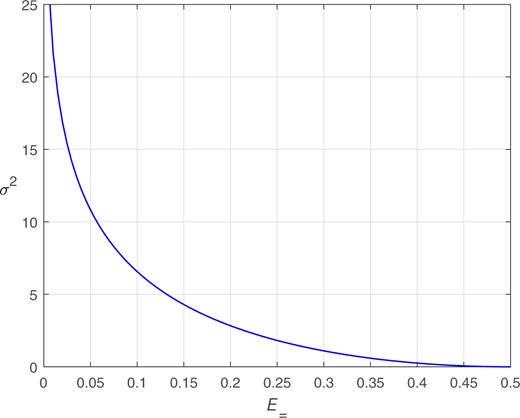
Relationship between and for a perfectly calibrated system.
2.6 Comparison of methods for determining the target value
In this subsection, we explore the performance of the alternative methods for determining the for the perfectly calibrated bi-Gaussian system toward which scores will be mapped (Steps 3 and 4 of the bi-Gaussianized-calibration method).
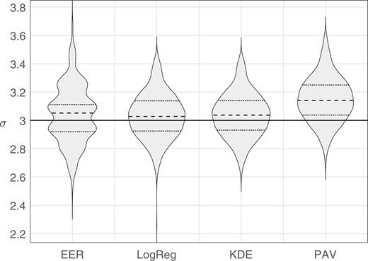
We generated synthetic data using Monte Carlo simulation. Sample sets consisting of 100 same-source scores and 4950 different-source scores were generated from perfectly calibrated bi-Gaussian systems with (the generating distributions are the same as those plotted in Fig. 3). For each value of , we generated 1,000 sample sets. For each sample set, we calculated the target value obtained from each method: EER, LogReg, KDE, and PAV. Violin plots of results are provided in Fig. 7 through Fig. 10, note that the scale of the y axis differs across figures. In each figure, the solid horizontal line indicates the “true” , that is, the parameter value used to generate the Monte Carlo samples. Table 1 gives the root-mean square (RMS) errors between the target value and the “true” value.
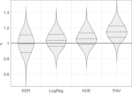
Violin plots of distributions of target values estimated by each method. The solid horizontal line indicates the parameter value used to generate the Monte Carlo samples, .
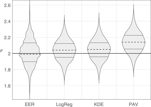
Violin plots of distributions of target values estimated by each method. The solid horizontal line indicates the parameter value used to generate the Monte Carlo samples, .
RMS errors of the target values obtained from each method relative to the “true” , the parameter value used to generate the Monte Carlo samples. For each “true” σ value, the RMS value for the best performing method is bolded.
| Methods | ||||
|---|---|---|---|---|
| “true” | EER | LogReg | KDE | PAV |
| 1 | 0.133 | 0.113 | 0.122 | 0.184 |
| 2 | 0.153 | 0.127 | 0.131 | 0.187 |
| 3 | 0.203 | 0.162 | 0.159 | 0.217 |
| 4 | 0.309 | 0.253 | 0.232 | 0.303 |
| Methods | ||||
|---|---|---|---|---|
| “true” | EER | LogReg | KDE | PAV |
| 1 | 0.133 | 0.113 | 0.122 | 0.184 |
| 2 | 0.153 | 0.127 | 0.131 | 0.187 |
| 3 | 0.203 | 0.162 | 0.159 | 0.217 |
| 4 | 0.309 | 0.253 | 0.232 | 0.303 |
The PAV method had a substantial bias toward larger target values than the “true” value. This is likely due to PAV overfitting the training data, resulting in smaller values and hence larger target values. Except for “true” , for which it had the second highest RMS error, the PAV method always had the highest RMS error. Because of the poor performance of PAV as a method for determining the target , in the remainder of the article, we do not make use of the PAV variant of the bi-Gaussianized-calibration method.
For the EER method, as the separation between the different-source distribution and the same-source distribution increases, sparsity of data in the overlapping tails of the distributions accounts for the multimodality in the distributions of target , that is, the multiple bulges see in the violin plots for the EER method for . Each bulge corresponds to a miss rate which, because there are only 100 same-source samples, is discretized into steps of 0.01, for example, for the EER method in Fig. 10, the highest bulge corresponds to a miss rate of 0.01, the middle (widest) bulge to a miss rate of 0.02, and the lowest bulge to a miss rate of 0.03, and in Fig. 9, the two widest bulges correspond to miss rates of 0.06 and 0.07. Except for “true” , for which it had the highest RMS error, the EER method always had the second highest RMS error.
Violin plots of distributions of target values estimated by each method. The solid horizontal line indicates the parameter value used to generate the Monte Carlo samples, .
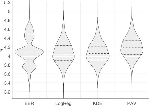
Violin plots of distributions of target values estimated by each method. The solid horizontal line indicates the parameter value used to generate the Monte Carlo samples, .
The RMS errors were consistently lowest for the LogReg and KDE methods. For “true” the LogReg method had the lowest RMS error, and for “true” the KDE method had the lowest RMS error. Both these methods had a slight bias toward larger target values than the “true” value (a somewhat greater bias for the KDE method when “true” ). This bias may be due to error in the procedure used to derive the to conversion function (Section 2.3), stochastic error, fitting error, or intrinsic underfitting due to an insufficiently complex regression equation.
Because the LogReg and KDE methods for determining the target result, on average, in target σ values that are closer to the “true” σ value than the EER and PAV methods, the LogReg and KDE variants of the bi-Gaussianized-calibration method appear to be more promising than the EER and PAV variants of the bi-Gaussianized-calibration method.
For the LogReg method when “true” , there was an outlier with a low value, which would result in a conservative calibration, that is, log-likelihood ratios closer to zero than for the “true” perfectly calibrate system. The KDE method does not exhibit an outlier, so this could be a reason to favor the KDE method over the LogReg method.
In order to have a “true” against which to compare target results, the Monte Carlo simulations used a different-source score distribution and a same-source score distribution which were Gaussian and had the same variance. In these simulations, the LogReg method’s assumption of linearity in the score (or ) domain was satisfied. When the different-source score distribution and the same-source score distribution are not Gaussian or do not have the same variance, and these assumptions are violated, it could be that the KDE variant of the bi-Gaussianized-calibration method will outperform the LogReg variant. Note that, although KDE as a calibration method would result in a non-linear mapping, when KDE is used to determine the target as part of the bi-Gaussianized-calibration method, the bi-Gaussianized-calibration method will result in a monotonic mapping.
2.7 Cumulative-distribution mapping
Step 5 of the bi-Gaussianized-calibration method requires determining the empirical cumulative distribution of the training scores output at Step 1. This is done giving equal weight to the set of different-source scores and the set of same-source scores (the number of different-source scores, , and the number of same-source scores, , usually differ). Each different-source score is given a weight of , and each same-source score is given a weight of . All the scores, , irrespective of their same-source or different-source labels, are sorted from smallest to largest, and the cumulative sums of the sorted scores’ weights are calculated. The resulting values of the cumulative sums of the weights monotonically increase from near 0 for the lowest-value score to near 1 for the highest-value score. In the denominators of the weights, the addition of 1 to and the addition of 1 to prevents the final cumulative-sum value from reaching 1. We define as the empirical-cumulative-distribution function. returns the value of the cumulative sum of the weights up to and including score value . If the score value, , is not exactly the same value as one of the training-score values, the value of is linearly interpolated using the closest training-score value below , the closest training-score value above , and their corresponding values. The method does not extrapolate beyond values encountered in the training data: If the value of is below the smallest score value in the training set or above the largest score value in the training set, the value returned by corresponds to, respectively, the value for the smallest score value in the training set or the value for the largest score value in the training set.
3. Demonstrations of the method
3.1 Introduction
We demonstrate application of the method using:
Synthetic score data for which the generating distributions are those of a perfectly-calibrated bi-Gaussian system (Section 3.2).
Synthetic score data for which the generating different-source distribution is Gaussian and the generating same-source distribution is skewed and has a smaller variance than the different-source distribution (Section 3.3).
Real score data from a forensic-voice-comparison system (Section 3.4). These data moderately deviate from the assumption of equal-variance Gaussians.
Real score data from a comparison of glass fragments (Section 3.5). These data exhibit extreme deviation from the assumption of equal-variance Gaussians.
For plots below of cumulative distributions, mapping functions, probability-density plots of values, and Tippett plots, we have always used the target obtained from the LogReg variant of bi-Gaussianized calibration. The target for the EER and KDE variants were always similar, so would have resulted in similar (often visually indistinguishable) plots.
3.2 Synthetic data: Equal-variance Gaussians
We generated synthetic data using Monte Carlo simulation. The generating different-source distribution was a Gaussian with parameters and , and the generating same-source distribution was a Gaussian with parameters and , that is, the perfectly calibrated bi-Gaussian system shown in Fig. 2a and in the third row of Fig. 3. We generated a training-data sample set consisting of 100 same-source scores and 4,950 different-source scores, and a separate test-data sample set of the same size.
In addition to applying bi-Gaussianized calibration (EER, LogReg, and KDE variants), we also applied LDF calibration using the Monte Carlo parameter values (which gives the “true” likelihood-ratio values), LogReg calibration, and PAV calibration.
The parameter value for was 3, and the target calculated for bi-Gaussianized calibration were 3.10, 2.96, and 2.95 for the EER, LogReg, and KDE variants, respectively. Figure 11 shows the empirical cumulative distribution for the score data, and the target cumulative distribution for a perfectly calibrated bi-Gaussian system with .
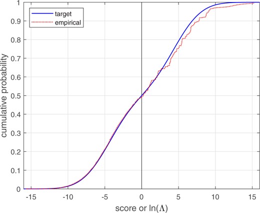
Empirical cumulative distribution of equal-variance Gaussian score data, and target cumulative distribution of a perfectly calibrated bi-Gaussian system with .
Figure 12 shows the “true” mapping function from scores to calibrated given the Monte Carlo population distributions. Since the Monte Carlo population distributions were a perfectly calibrated bi-Gaussian system, the “true” mapping function is the identity function. Figure 12 also shows the mapping functions from scores to calibrated for PAV, LogReg, and bi-Gaussianized calibration (with target ). LogReg calibration results in a linear mapping which is close to the perfect-calibration line. PAV calibration results in a stepped mapping function in which some steps are large and have relatively large deviations from the perfect-calibration line. Below the smallest same-source score and above the largest different-source score in the training data, the PAV mapping ceases to change, resulting in even larger deviations from the perfect-calibration line. In contrast to PAV calibration, bi-Gaussianized calibration results in a smoother mapping that generally stays closer to the perfect-calibration line, including below the smallest same-source score and above the largest different-source score in the training data.
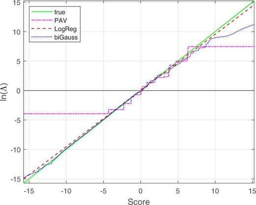
Mapping functions from scores to calibrated for the synthetic equal-variance Gaussian score data. The bi-Gaussianized-calibration mapping is for target .
Table 2 gives the values for LDF calibration using the Monte Carlo population distributions (“true” values), bi-Gaussianized calibration, LogReg calibration, and PAV calibration. All methods, other then PAV calibration, resulted in similar values (by design, the value for the LogReg variant of bi-Gaussianized calibration should be approximately the same as that for LogReg calibration). PAV calibration exhibited overfitting on the training data: it had the lowest value on the training data but the highest on the test data. Compared to PAV calibration, bi-Gaussianized calibration exhibited less overfitting.
values for different calibration methods applied to the synthetic equal-variance Gaussian data.
| Method | ||||||
|---|---|---|---|---|---|---|
| “true” | Bi-Gauss | LogReg | PAV | |||
| Data | EER | LogReg | KDE | |||
| train | 0.251 | 0.249 | 0.248 | 0.248 | 0.251 | 0.231 |
| test | 0.212 | 0.213 | 0.216 | 0.216 | 0.213 | 0.220 |
| Method | ||||||
|---|---|---|---|---|---|---|
| “true” | Bi-Gauss | LogReg | PAV | |||
| Data | EER | LogReg | KDE | |||
| train | 0.251 | 0.249 | 0.248 | 0.248 | 0.251 | 0.231 |
| test | 0.212 | 0.213 | 0.216 | 0.216 | 0.213 | 0.220 |
3.3 Synthetic data: Gaussian distribution and skewed distribution with smaller variance
We generated synthetic data using Monte Carlo simulation. The generating different-source distribution was a Gaussian with parameters and , and the generating same-source distribution was a Gumbel distribution with parameters and that was mirrored about 0, see Fig. 13. These are similar to distributions sometimes observed for real score data. We generated a training-data sample consisting of 100 same-source scores and 4,950 different-source scores, and a separate test-data sample of the same size.

Distributions used for Monte Carlo simulation: Gaussian distribution and skewed distribution with smaller variance.
In addition to applying bi-Gaussianized calibration (EER, LogReg, and KDE variants), we also used the Monte Carlo generating distributions to calculate “true” likelihood-ratio values, and applied LogReg calibration, and PAV calibration.
The calculated target for bi-Gaussianized calibration were 3.65, 3.65, and 3.72 for the EER, LogReg, and KDE variants, respectively. Figure 14 shows the empirical cumulative distribution for the score data, and the target cumulative distribution for a perfectly calibrated bi-Gaussian system with .
Empirical cumulative distribution of Gaussian and skewed-distribution score data, and target cumulative distribution of a perfectly calibrated bi-Gaussian system with .
Figure 15 shows the “true” mapping function from scores to calibrated given the Monte Carlo population distributions. Figure 15 also shows the mapping functions from scores to calibrated for PAV, LogReg, and bi-Gaussianized calibration (with target ). For low and high score values, the “true” mapping is non monotonic. This is an artifact of the population distributions chosen. Score to calibrated mappings for real data should be monotonic. References to “true” mapping in the remainder of this paragraph are with respect to its central monotonically increasing range (between score values of about –8 and +9). LogReg calibration results in a linear mapping which is close to the “true” mapping. PAV calibration results in a stepped mapping function in which the larger steps have relatively large deviations from the “true” mapping. In contrast to PAV calibration, bi-Gaussianized calibration results in a smoother mapping that generally stays closer to the “true” mapping. At low score values, the bi-Gaussianized calibration pulls the values closer to 0 than does logistic regression, and at high score values, the bi-Gaussianized calibration pushes the values further from 0 than does logistic regression.
Mapping functions from scores to calibrated for the synthetic Gaussian and skewed-distribution score data. The bi-Gaussianized-calibration mapping is for target . The scale and range of the x-axis on this plot is the same as for the plot of the different-source and same-source distributions in Fig. 13.
Figures 16 and 17 show the different-source and same-source distributions for the training data and the test data, respectively. The solid lines show the target distributions, the distributions for a perfectly calibrated bi-Gaussian system with . Kernel-density plots are used to draw the LogReg and bi-Gaussianized calibration distributions. LogReg calibration only involves shifting and scaling in the space, and the resulting distributions are shifted and scaled versions of the distributions of samples taken from the population distributions shown in Fig. 13. These LogReg calibrated distributions are relatively far from those of the perfectly calibrated bi-Gaussian target distributions. In contrast, bi-Gaussianized calibration involves non-linear (but still monotonic) warping, resulting in distributions that are much closer to those of the perfectly calibrated bi-Gaussian target distributions. Although the bi-Gaussianized calibrated distributions for the training data (Fig. 16) are due to training and testing on the same data, they are not perfect matches for the target distributions. This is because the bi-Gaussianized calibration mapping function is trained without the use of same-source and different-source labels. The bi-Gaussianized calibrated distributions for the test data (Fig. 17) are further from those of the perfectly calibrated bi-Gaussian target than are those for the training data (Fig. 16), but they are still much closer to the perfectly calibrated bi-Gaussian target distributions that are the LogReg calibrated distributions.
Different-source and same-source distributions of calibrated for the synthetic Gaussian and skewed-distribution score data. The target and bi-Gaussianized distributions are for target . Training data.
Different-source and same-source distributions of calibrated for the synthetic Gaussian and skewed-distribution score data. The target and bi-Gaussianized distributions are for target . Test data.
Table 3 gives the “true” values calculated using the Monte Carlo population distributions, and values for bi-Gaussianized calibration, LogReg calibration, and PAV calibration. All methods resulted in similar values, except for PAV calibration, which, due to overfitting, had a lower on the training data.
values for different calibration methods applied to the Gaussian and skewed-distribution data.
| Method | ||||||
|---|---|---|---|---|---|---|
| “true” | Bi-Gauss | LogReg | PAV | |||
| Data | EER | LogReg | KDE | |||
| train | 0.127 | 0.129 | 0.129 | 0.129 | 0.126 | 0.113 |
| test | 0.138 | 0.140 | 0.140 | 0.140 | 0.134 | 0.137 |
| Method | ||||||
|---|---|---|---|---|---|---|
| “true” | Bi-Gauss | LogReg | PAV | |||
| Data | EER | LogReg | KDE | |||
| train | 0.127 | 0.129 | 0.129 | 0.129 | 0.126 | 0.113 |
| test | 0.138 | 0.140 | 0.140 | 0.140 | 0.134 | 0.137 |
Figure 18 shows the Tippett plots for the target perfectly calibrated system, and for the logistic-regression and bi-Gaussianized calibrated likelihood-ratio values for the test data.14 The bi-Gaussianized calibrated results are closer to the target perfectly calibrated bi-Gaussian system than are the logistic-regression calibrated results. This is because, as mentioned above in relation to Fig. 15, at low score values, the bi-Gaussianized calibration pulls the values closer to 0 than does logistic regression, and at high score values, the bi-Gaussianized calibration pushes the values further from 0 than does logistic regression.
Tippett plots for the target perfectly calibrated system with , and for the LogReg calibrated and bi-Gaussianized calibrated likelihood-ratio values. Synthetic Gaussian and skewed-distribution score data. Test data.
One should note that the curves representing the perfectly calibrated bi-Gaussian system in Figs 16–18 (and parallel figures in subsections below) do not represent the distributions of “true” likelihood ratios, which (except in the context of Monte Carlo simulation) are unknown and unknowable. All three systems represented in these figures (LogReg, bi-Gaussianized, and perfect calibration) have, by design, (approximately) the same for the training data. The comparisons between the different systems that these figures allow are comparisons of how well calibrated the likelihood-ratio outputs of different systems with (approximately) the same are. It is not a comparison of the likelihood-ratio outputs of different systems with “true” likelihood ratios. Given two different systems with (approximately) the same , and so equally good performance on this metric, we argue that the better of the two systems is the system which is closer to a perfectly calibrated system with that .15 If one accepts this argument, then Figs 16–18 (and parallel figures in subsections below) show that bi-Gaussianized calibration is better than LogReg calibration.
3.4 Real data: Forensic voice comparison
Real score data were taken from the E3 Forensic Speech Science System (E3FS3) and applied to the benchmark forensic-eval_01 data, see Weber et al. (2022).16 There were 111 same-source scores and 9719 different-source scores originating from a total of 223 recordings of 61 speakers. Kernel-density plots of the different-source and same-source score distributions are shown in Fig. 19. These data clearly deviate from the assumption of equal-variance Gaussians (although one may consider this a moderate deviation).
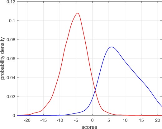
Kernel-density plots of the different-source and same-source score distributions from comparison of voice recordings.
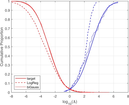
We applied bi-Gaussianized calibration (EER, LogReg, and KDE variants), LogReg calibration, and PAV calibration using leave-one-out/leave-two-out cross-validation.17 Over cross-validation loops, the mean target for bi-Gaussianized calibration was 3.75, 3.44, and 3.45 for the EER, LogReg, and KDE variants respectively. Figure 20 shows the empirical cumulative distribution for the score data, and the target cumulative distribution for a perfectly calibrated bi-Gaussian system with . The mapping functions are shown in Fig. 21. Relative to the logistic-regression mapping, the bi-Gaussianized calibration mapping pulls both large negative scores and moderate-to-large positive scores closer to .
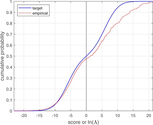
Empirical cumulative distribution of voice-comparison score data, and target cumulative distribution of a perfectly calibrated bi-Gaussian system with . The scale and range of the x-axis on this plot is the same as for the plot of the different-source and same-source distributions in Fig. 19.
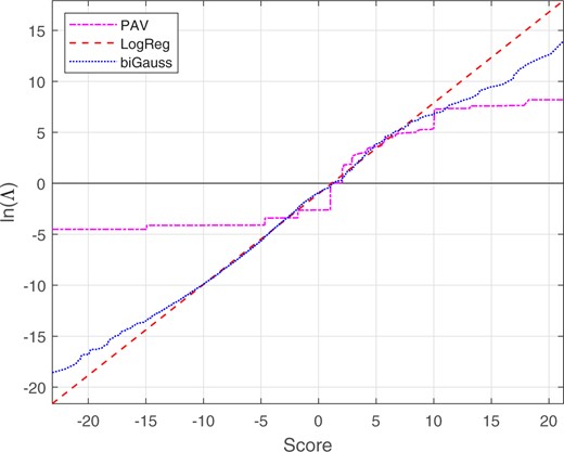
Mapping functions from scores to calibrated for the voice-comparison score data. The bi-Gaussianized-calibration mapping is for target . The scale and range of the x-axis on this plot is the same as for the plot of the different-source and same-source distributions in Fig. 19.
Figure 22 shows the different-source and same-source distributions. The solid lines show the target distributions, the distributions for a perfectly calibrated bi-Gaussian system with . Kernel-density plots are used to draw the logistic-regression and bi-Gaussianized calibration distributions. Figure 23 shows the corresponding Tippett plots. In both the probability-density plots and the Tippett plots, it can be seen that the bi-Gaussianized calibration results are closer to the perfectly calibrated bi-Gaussian system than are the logistic-regression calibration results. The logistic-regression calibration results deviate particularly for moderate-to-large log-likelihood-ratio values, these log-likelihood-ratio values are higher than for the perfectly calibrated bi-Gaussian system.
Different-source and same-source distributions of calibrated for the voice-comparison score data. The target and bi-Gaussianized distributions are for target .
Tippett plots for the target perfectly calibrated system with , and for the LogReg and bi-Gaussianized calibrated likelihood-ratio values. Voice-comparison score data.
Table 4 gives the values resulting from the application of bi-Gaussianized calibration (EER, LogReg, and KDE variants), LogReg calibration, and PAV calibration. All the values were approximately the same.
values for different calibration methods applied to the speaker data.
| Method | ||||
|---|---|---|---|---|
| Bi-Gauss | LogReg | PAV | ||
| EER | LogReg | KDE | ||
| 0.171 | 0.172 | 0.171 | 0.172 | 0.168 |
| Method | ||||
|---|---|---|---|---|
| Bi-Gauss | LogReg | PAV | ||
| EER | LogReg | KDE | ||
| 0.171 | 0.172 | 0.171 | 0.172 | 0.168 |
3.5 Real data: Glass fragments
Real score data were taken from comparison of glass fragments by Vergeer et al. (2016) and van Es et al. (2017).18 The glass-fragment data consisted of multiple fragments from each of 320 sources, resulting in 320 same-source scores and 51,040 different-source scores. Due to numerical limitations in the software that calculated the scores, 41,108 (∼80%) of the different-source scores had a value of –∞. We converted the value of these scores to the lowest finite score value that already existed in the dataset, thus producing a probability mass at that value. Kernel-density plots of the different-source and same-source score distributions are shown in Fig. 24.19 The different-source distribution has a point mass at approximately –300, and probability density spread between –300 and 6.5. Apart from a few outliers, the same-source density is concentrated in a relatively narrow range of low positive values, with the mode at 9.0. The different-source and same-source scores overlap in the range –1.7 to 6.5. These distributions exhibit extreme deviation from the assumption of equal-variance Gaussians.
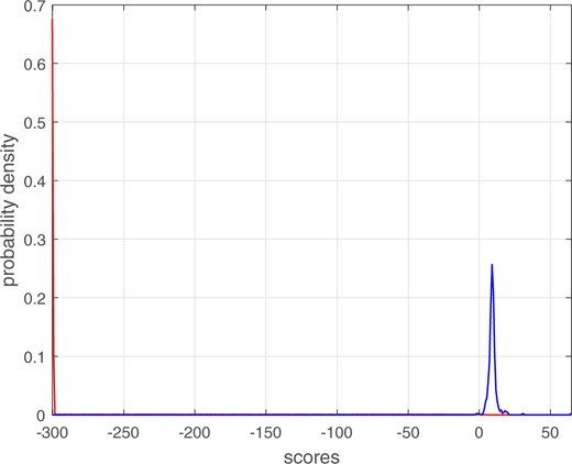
Kernel-density plots of the different-source and same-source score distributions from comparison of glass fragments.
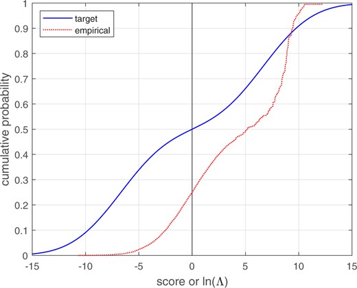
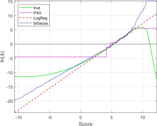
We applied bi-Gaussianized, LogReg, and PAV calibration using leave-one-out/leave-two-out cross-validation.20 Averaged over cross-validation loops, the target for bi-Gaussianized calibration were 5.65, 6.02, and 6.01 for the EER, LogReg, and KDE variants respectively. Figure 25 shows the empirical cumulative distribution for the score data, and the target cumulative distribution for a perfectly calibrated bi-Gaussian system with . The probability mass accounting for ∼80% of the different-source-scores results in the empirical distribution beginning at ∼0.4. The mapping functions are shown in Figs 26 and 27 (Fig. 27 shows details of Fig. 26 around the range of values in which the different-source and same-source scores overlap). Whereas the LogReg mapping is linear and maps to a broad range of values, the bi-Gaussianized calibration mapping is sigmoidal and maps to a much narrower range of values. Whereas, outside the range of values in which the different-source and same-source scores overlap (–1.7 to 6.5), the PAV mapping is flat, the bi-Gaussianized calibration mapping has monotonically increasing slopes which reach below and above the minimum and maximum PAV-mapped values. Far from the overlap range, those slopes are shallow. In the range of values in which the different-source and same-source scores overlap (–1.7 to 6.5), the bi-Gaussianized calibration mapping and the PAV mapping are close to each other, but the bi-Gaussianized calibration mapping is smoother.21
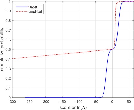
Empirical cumulative distribution of glass-fragment score data, and target cumulative distribution of a perfectly calibrated bi-Gaussian system with . The scale and range of the x-axis on this plot is the same as for the plot of the different-source and same-source distributions in Fig. 24.
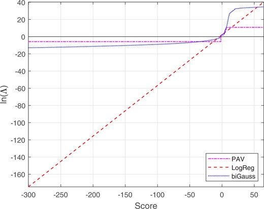
Mapping functions from scores to calibrated for the glass-fragment score data. The bi-Gaussianized-calibration mapping is for target . The scale and range of the x-axis on this plot is the same as for the plot of the different-source and same-source distributions in Fig. 24.
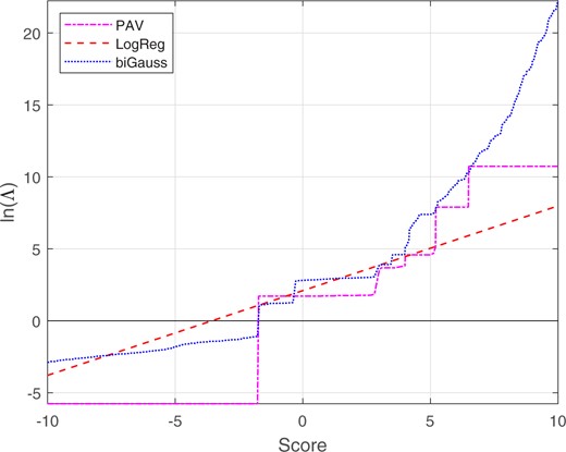
Part of the mapping functions from scores to calibrated for the glass-fragment score data (part of Fig. 26), showing details around the range of values in which the different-source and same-source scores overlap (–1.7 to 6.5).
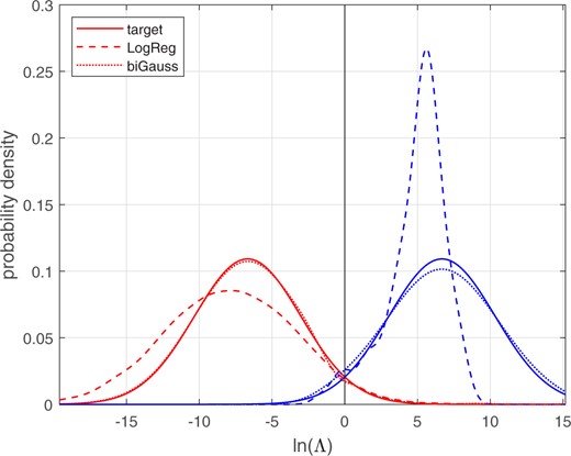
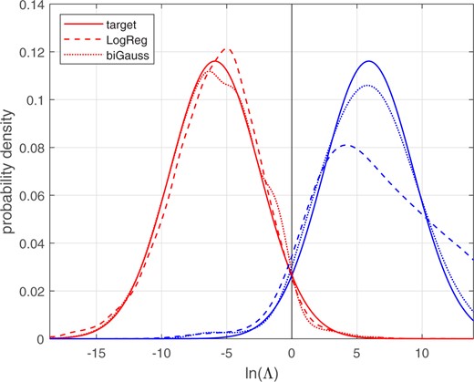
Figure 28 shows the different-source and same-source distributions. The solid lines show the target distributions, the distributions for a perfectly calibrated bi-Gaussian system with . Kernel-density plots were used to draw the LogReg and bi-Gaussianized calibrated distributions. For the different-source bi-Gaussianized calibration distribution, the probability mass, which is at , is represented as a spike (the probability-density axis is truncated at 0.5, the spike reaches much higher).22 The remainder of the different-source bi-Gaussianized distribution is represented as a curve to the right of the spike, which is mostly obscured by the different-source curve of the target bi-Gaussian distribution. The different-source LogReg calibrated distribution rises very slowly, and eventually has a probability mass at (outside the range of plotted values). Other than at their probability mass, the bi-Gaussianized calibration results are much closer to perfectly calibrated bi-Gaussian target distributions than are the LogReg calibration results.
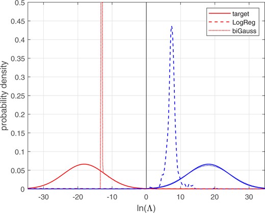
Different-source and same-source distributions of calibrated for the glass-fragment score data.
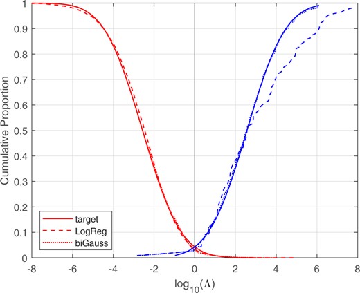
Figure 29 shows the Tippett plots. The vertical part of the different-source curve for the bi-Gaussianized calibration (at ) is due to the probability mass, otherwise, the bi-Gaussianized calibration curves lie almost directly on top of the perfectly calibrated bi-Gaussian target curves (and are mostly obscured by the latter). In contrast, the LogReg calibration curves are generally far from the perfectly calibrated bi-Gaussian target curves.
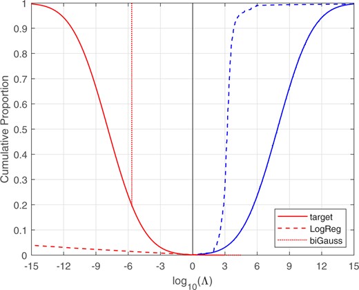
Tippett plots for the target perfectly calibrated system with , and for the LogReg and bi-Gaussianized calibrated likelihood-ratio values. Glass-fragment score data.
For the bi-Gaussianized calibration, the probability mass occurs at , which is a likelihood ratio of approximately 468,000 in favor of the different-source hypothesis. One could report that the likelihood ratio is at least 468,000 in favor of the different-source hypothesis.
Table 5 gives the values resulting from the application of bi-Gaussianized calibration (EER, LogReg, and KDE variants), LogReg calibration, and PAV calibration. All the values were approximately the same.
values for different calibration methods applied to the glass data.
| Method | ||||
|---|---|---|---|---|
| Bi-Gauss | LogReg | PAV | ||
| EER | LogReg | KDE | ||
| 0.006 | 0.005 | 0.005 | 0.006 | 0.006 |
| Method | ||||
|---|---|---|---|---|
| Bi-Gauss | LogReg | PAV | ||
| EER | LogReg | KDE | ||
| 0.006 | 0.005 | 0.005 | 0.006 | 0.006 |
The maximum likelihood-ratio value generated by bi-Gaussianized calibration was very large, 1.05 × 10¹⁵. Concerns over whether such large likelihood-ratio values are justified given relatively limited amounts of training data have led to proposals that the reported values of likelihood ratios be limited in size or that they be shrunk toward the neutral value of 1. Vergeer et al. (2016) proposed a method to limit likelihood-ratio values, Empirical Lower and Upper Bounds (ELUB), which when applied to the same glass data as in the article limited to the range −2.50 to 4.53.23 Smaller calculated values would be replaced by , and larger calculated values would be replaced by . Morrison and Poh (2018) proposed a method to shrink log-likelihood-ratio values toward 0 by using a large regularization weight for regularized-logistic-regression calibration. The latter method could be applied in the LogReg variant of bi-Gaussianized calibration and would result in a smaller target value than if no regularization were applied or if a small regularization weight were used (this article used a small regularization weight). Bi-Gaussianized calibration potentially offers another method for inducing shrinkage: The magnitude of the target value could be reduced from its calculated value, for example, it could be reduced to 90% of the value calculated using Equation (8) or Equation (10). This would result in the bi-Gaussianized calibrated log-likelihood ratios being closer to 0 than would otherwise be the case. As with other methods for inducing shrinkage, one would have to make a choice as to how much shrinkage to induce (a choice which should make reference to the amount of training data used). Note also, that inducing substantial shrinkage leads to larger . We do not explore this shrinkage method in the present paper.
4. Effect of sampling variability
In Section 3, the bi-Gaussianized calibration method was demonstrated using four different data sets (two simulated and two real). Each dataset was treated as a sample from a relevant population. Different samples from the same population would be expected to produce different results. In the present section, we explore the effect of sampling variability on the output of bi-Gaussianized, LogReg, and PAV calibration. Smaller samples would be expected to result in greater sampling variability, and the size of case-relevant samples that can practically be obtained in the context of forensic cases is often small. In addition to testing samples of 100 sources (as for the Monte Carlo simulations in Sections 3.2 and 3.3), we also test samples of 50 sources.
As in Section 3.2, we generated synthetic data using Monte Carlo simulation. The generating different-source distribution was a Gaussian with parameters and , and the generating same-source distribution was a Gaussian with parameters and , that is, the perfectly calibrated bi-Gaussian system shown in Fig. 2a and in the third row of Fig. 3. We generated a single test-data sample set consisting of 10,000 same-source scores and 10,000 different-source scores. By using a single large balanced test set, we can attribute any bias and variability in the results to bias in the calibration methods and sampling variability in the training sets. We generated 1,000 training-data sample sets, each consisting of 100 same-source scores and 4,950 different-source scores (the 100 source datasets), and another 1,000 training-data sample sets, each consisting of 50 same-source scores and 1,225 different-source scores (the 50 source datasets). For each training-data sample set, we calibrated the test-data sample set using bi-Gaussianized calibration (EER, LogReg, and KDE variants), LogReg calibration, and PAV calibration, and calculated the for the resulting sets of .
Figures 30 and 31 show violin plots of the distributions of values for the 100 source datasets, and Figs 32 and 33 show violin plots of the distributions of values for the 50 source datasets. The first figure in each pair uses a range of 0 to 1, giving an impression of the distributions of values relative to the possible range of for well-calibrated systems. The second figure in each pair zooms in to show the shapes of the distributions—note that the range of values on the y axis of Fig. 33 is twice that of Fig. 31. In each figure, the solid horizontal line represents the “true” value, 0.241, which corresponds to a perfectly calibrated bi-Gaussian system with .24
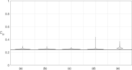
Violin plots of distributions of target values resulting from the application of different calibration methods using 1,000 training-data sample sets (100 source datasets). (a) Bi-Gaussianized calibration EER variant. (b) Bi-Gaussianized calibration LogReg variant. (c) Bi-Gaussianized calibration KDE variant. (d) LogReg calibration. (d) PAV calibration. The solid horizontal line represents the “true” .
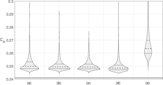
Violin plots of distributions of target values resulting from the application of different calibration methods using 1,000 training-data sample sets (100 source datasets). (a) Bi-Gaussianized calibration EER variant. (b) Bi-Gaussianized calibration LogReg variant. (c) Bi-Gaussianized calibration KDE variant. (d) LogReg calibration. (e) PAV calibration. The solid horizontal line represents the “true” .
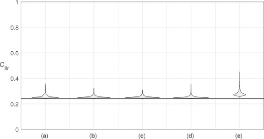
Violin plots of distributions of target values resulting from the application of different calibration methods using 1,000 training-data sample sets (50 source datasets). (a) Bi-Gaussianized calibration EER variant. (b) Bi-Gaussianized calibration LogReg variant. (c) Bi-Gaussianized calibration KDE variant. (d) LogReg calibration. (e) PAV calibration. The solid horizontal line represents the “true” .
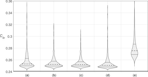
Violin plots of distributions of target values resulting from the application of different calibration methods using 1,000 training-data sample sets (50 source datasets). (a) Bi-Gaussianized calibration EER variant. (b) Bi-Gaussianized calibration LogReg variant. (c) Bi-Gaussianized calibration KDE variant. (d) LogReg calibration. (e) PAV calibration. The solid horizontal line represents the “true” .
For all calibration methods and all training-data samples, calculated was greater than the “true” , that is, no sample-based method outperformed a calculation based on the population’s parameter values. With the exception of PAV calibration and of a few outliers, however, all calculated were only a little higher than the “true” . As would be expected, calculated values tended to be higher for the 50 source datasets than for the 100 source datasets.
The highest values (the worst performance) occurred for PAV calibration—PAV overfits the training data. For bi-Gaussianized calibration, the median and quartile values were similar across variants, but were slightly higher for the EER variant, than for the LogReg variant, and slightly higher for the LogReg variant than for the KDE variant. Also, outliers were most extreme for the EER variant, less extreme for the LogReg variant, and least extreme for the KDE variant. For LogReg calibration, the median and quartile were slightly lower than for the KDE variant of bi-Gaussianized calibration, but it produced much more extreme outliers. Even though, by design, on the training data, the LogReg variant of bi-Gaussianized calibration should have (approximately) the same as LogReg calibration, on the test data, outliers for the LogReg variant of bi-Gaussianized calibration were not as extreme as for LogReg calibration.
Based on these results, the KDE variant appears to be the best-performing variant of bi-Gaussianized calibration. Taking into account the outliers in these results, the KDE variant of bi-Gaussianized calibration also appears to be a better choice than LogReg calibration.
We separately ran the 1,000 training datasets (100 source versions) for each variant of bi-Gaussianized calibration, and for LogReg calibration, and timed how long each took (including the time to generate the training data). On the particular machine we used (using three parallel workers), the EER variant took 5.8 s, the LogReg variant took 7.8 s, the KDE variant took 131 s, and LogReg calibration took 3.3 s. A disadvantage of the KDE variant of bi-Gaussianized calibration, therefore, is that it takes much longer than the other variants of bi-Gaussianized calibration and much longer than LogReg calibration. If time were an issue, the LogReg variant of bi-Gaussianized calibration might be a better choice than the KDE variant.
5. Graphical representation of likelihood-ratio output
A biproduct of bi-Gaussianized calibration is that it provides a way of graphically representing results which may aid in explaining them to triers of fact or to other interested parties. Since logistic regression is a discriminative method, rather than a generative method, it does not actually calculate the ratio of two likelihoods, thus the output of LogReg calibration cannot be directly graphically represented as the relative heights of two probability-density curves. If one has used bi-Gaussianized calibration, however, one can plot the same-source target probability-density function and the different-source target probability-density function, and graphically show the relative height of the two curves at a value of interest.
Figure 34 provides an example using a perfectly calibrated system with . One can explain that the better the performance of the system under the conditions of the case,25 the further apart the different-source and the same-source curves will be, that is, the less overlap there will be between the two curves. The x-axis is labeled “likelihood ratio.” This axis has a logarithmic scale, but the values along the axis are written in linear form. Imagine that the likelihood-ratio value calculated for the comparison of the questioned- and known-source items was 10. We find the corresponding location on the x-axis, and draw a vertical line that intersects the same-source probability-density curve and the different-source probability-density curve. We highlight the intersect points and draw horizontal lines from the intersect points to the y-axis. The y-axis is labeled “relative likelihood,” and is scaled so that the relative likelihood of the lowest of the two aforementioned intersects has a value of 1.26 In this example, the y-axis is scaled so that the intersect with the different-source curve has a relative-likelihood value of 1. In this example, given this scaling, the intersect with the same-source curve has a relative-likelihood value of 10. It is then easy to explain that, for the reported likelihood-ratio value for the comparison of the questioned- and known-source items, the relative likelihood for obtaining that value if the same-source hypothesis were true is times greater than the relative likelihood for obtaining that value if the different-source hypothesis were true, which is what the reported likelihood-ratio value on the x axis means. This will work for any likelihood-ratio value selected on the x-axis. We leave it as a task for future research to assess whether graphics of this form will actually be helpful for explaining the meaning of likelihood ratios to triers of fact.
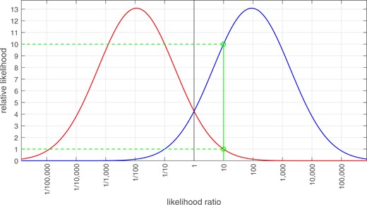
Example graphic designed for communicating the meaning of a likelihood-ratio value.
6. Conclusion
For the output of a perfectly calibrated forensic evaluation system, the likelihood ratio of the likelihood ratio is the likelihood ratio. If the distributions of the different-source and same-source natural-log-likelihood ratios, , output by the system are both Gaussian and they have the same variance, , and the different-source and same-source means are and , then the output of the system is perfectly calibrated—this is a perfectly calibrated bi-Gaussian system.
Uncalibrated log-likelihood ratios (scores) are often calibrated using logistic regression (LogReg), but, unless the score distributions consist of two Gaussians with equal variance, the resulting “calibrated” can be far from perfectly calibrated. We proposed a new calibration method, “bi-Gaussianized calibration,” that maps scores toward perfectly calibrated bi-Gaussian distributions. The particular perfectly calibrated bi-Gaussian system that the scores are mapped toward, is the perfectly calibrated bi-Gaussian system with either the same equal-error rate (, EER) as the training data, or the same as the training data after they are calibrated using either LogReg, KDE, or PAVs. The method requires calculating the value for the perfectly calibrated bi-Gaussian system that corresponds to the or calculated for the training data. We found that the PAV method resulted in biased target values. The EER, LogReg, and KDE methods exhibited less bias and all resulted in similar target values.
We demonstrated the application of bi-Gaussianized calibration using two sets of simulated data and two sets of real data, including real data with extreme deviation from the assumption that same-source scores and different-source scores are distributed as two Gaussians with the same variance. The demonstrations showed that:
Bi-Gaussianized calibration is robust to deviation from the assumption that the scores are distributed as two Gaussians with the same variance.
Bi-Gaussianized calibration results in smoother score to mapping functions than PAV calibration, and, for simulated data, bi-Gaussianized calibration results in mapping functions that are closer to “true” mapping functions than does PAV calibration.
Bi-Gaussianized calibration results in values that are closer to a perfectly calibrated bi-Gaussian system than is the case for values output by LogReg calibration.
We introduced an innovation in drawing Tippett plots in which, in addition to the empirical results, we included the cumulative-density functions for the target perfectly calibrated bi-Gaussian system. This allows for comparison of the empirical results (e.g., bi-Gaussianized calibration results or LogReg calibration results) with the perfectly calibrated bi-Gaussian system with (approximately) the same .
We argued that if two calibration methods result in (approximately) the same value when applied to the same data (as is the case for bi-Gaussianized calibration and LogReg calibration), the better system is the one whose outputs are closer to the perfectly calibrated system with that value, that is, in our results, in terms of degree of calibration, bi-Gaussianized calibration was better than LogReg calibration.
Using simulated data to explore the effect of sampling variability on the performance of calibration methods, we found that:
PAV calibration tended to result in higher values (worse performance) than other calibration methods.
The EER, LogReg, and KDE variants of bi-Gaussianized calibration, and LogReg calibration, all resulted in similar median and quartile values.
The KDE variant of bi-Gaussianized calibration had less extreme outlier values than the other variants of bi-Gaussianized calibration and than LogReg calibration.
In terms of performance as measured by and in terms of degree of calibration, the KDE variant of bi-Gaussianized calibration therefore appears to be the best of the variants and methods tested. It does, however, take many times longer to run than other variants of bi-Gaussianized calibration and than LogReg calibration. If time were an issue, the LogReg variant of bi-Gaussianized calibration might be a better choice.
As with all calibration methods, it is important to use training data for bi-Gaussianized calibration that are representative of the relevant population and reflective of the conditions for the case. This includes having sufficiently large training sets; otherwise, there is a danger of overfitting the training data and not generalizing well to validation data or to the actual questioned- and known-source items from the case. Depending on one’s tolerance for such overfitting, the results of exploring the effect of sampling variability suggested that training data from 50 to 100 items may be acceptable.
We mentioned that, if one were concerned about calculating very large magnitude log-likelihood ratios on the basis of a limited amount of training data, in bi-Gaussianized calibration, one could induce shrinkage of log-likelihood ratios toward the neutral value of 0 by using a smaller for the target perfectly calibrated bi-Gaussian system than the calculated target value.
Finally, we proposed a graphical representation which may help in explaining the meaning of likelihood ratios to triers of fact. This displays the value of the likelihood ratio of interest on the probability-density plots of the target perfectly calibrated bi-Gaussian system. Whether this actually does assist with explaining the meaning of likelihood ratios is a question for future research.
Disclaimer
All opinions expressed in this article are those of the author, and, unless explicitly stated otherwise, should not be construed as representing the policies or positions of any organizations with which the author is associated.
Declaration of competing interest
The author declares that they have no known competing financial interests or personal relationships that could have appeared to influence the work reported in this article.
Footnotes
Good (1985) p. 257 attributes the discovery of this relationship to Turing.
For explanations of and of Tippett plots, see Morrison et al. (2021) Appendix C.
Morrison & Enzinger (2018), Neumann & Ausdemore (2020), and Neumann et al. (2020) have argued that calculating likelihood ratios based on scores that only take account of similarity does not result in meaningful likelihood-ratio values because they do not take account of typicality with respect to the relevant population for the case. Vergeer (2023), however, argues that use of similarity-score-based systems to calculate likelihood ratios is acceptable if system performance is better than using prior odds.
Laplace’s rule of succession can be used to prevent the values outside this range from being reported as –∞ and +∞, see Brümmer & du Preez (2006) §13.2.1.1.
We use a regularized version of logistic regression with a regularization weight of relative to the number of sources, see Morrison & Poh (2018) for details. This amount of regularization resolves potential numerical problems, but does not induce substantial shrinkage.
We used Gaussian kernels with the bandwidth determined using the Gaussian-approximation method, aka Silverman’s rule of thumb (Silverman, 1986, p. 45).
For PAV, we used Laplace’s rule of succession so that score values below the smallest same-source score and score values above the largest different-source score result in finite values (see note 4 above).
The form of Equation (5) is that given in González-Rodríguez et al. (2007) and thereafter widely repeated in the literature. It can be derived from Brümmer & du Preez (2006) Equation 43.
In general, a sum converts to an integral , in which is the probability density function for , and is the function of for which one wishes to integrate out .
We used the “integral” function in Matlab®.
The general form of the equation would be , but at , , therefore .
If FAR became less than MR because of a step up in MR, FAR had the same value at that datapoint and at the immediately preceding datapoint. If FAR became less than MR because of a step down in FAR, MR had the same value at that datapoint and at the immediately preceding datapoint.
is defined differently in Equation (11) than in Equation (10).
For the calculation of the cumulative proportions for Tippett plots, we used denominators of and rather than and . This prevents the maximum cumulative proportion from reaching 1, which is appropriate for plotting the cumulative-density functions and for the distributions of the perfectly calibrated system. and would only occur when and , respectively. The x axes of Tippett plots are scaled in base-ten logarithms rather then natural logarithms, but this is simply a difference in scaling.
The family of perfectly calibrated systems of distributions that we have chosen to use is bi-Gaussian systems. If we had chosen some other family of perfectly calibrated systems, our method would have mapped the test data toward the distributions of the member of that family with the corresponding to that of the training data after the initial calibration step.
The version of E3FS3 used was a later version than that used in Weber et al. (2022) and had slightly better performance. For display purposes, we rescaled the score values to 2.5% of their raw values. This linear rescaling has no impact on the results of subsequent application of calibration methods.
For a same-source comparison, all scores from comparisons that involved the source contributing to the score being calibrated were excluded from training. For a different-source comparison, all scores from comparisons that involved either or both of the sources contributing to the score being calibrated were excluded from training.
The glass score data were kindly provided by Peter Vergeer of the Netherlands Forensic Institute. The scores had been calculated using the multivariate-kernel-density method of Aitken & Lucy (2004). The raw data (as opposed to the scores) are available from: https://github.com/NetherlandsForensicInstitute/elemental_composition_glass
To plot the KDEs in Figure 24, the Gaussian-approximation method was used to determine the bandwidth to use for the same-source scores, then that same bandwidth was used for the different-source scores.
Because otherwise the cross-validation would have taken an extremely long time, we excluded test scores that had been –∞. Scores that had been –∞ (and had been converted to the lowest finite score value in the dataset) were, however, still included in training. We then assigned the lowest value calculated for a finite test scores as the value corresponding to all the test scores that had been –∞. Had we included the test scores that had been –∞ in the cross-validation, because of differences in training data from loop to loop, each would have resulted in a slightly different value. On the particular machine, we used (using 19 parallel workers), it took 11 hours to run the cross-validation.
The larger steps in the bi-Gaussianized calibration’s mapping function are due to sparce same-source scores. The first three same-source scores occur at −1.7, −0.3, and 3.0, which correspond to the end of the rise of the first large step up, the second large step up, and the step up following the second large stepup.
To represent the probability mass as a spike, the bandwidth of the kernel for the different-source distribution was manually set to 0.1.
The bounds are calculated after a calibration model has been applied, so their values will depend on the particular calibration model used. These particular values were the result of calibration that fitted a KDE to the different-source scores and a double-exponential model to the same-source scores.
The value was calculated using Equation (7).
The system should have been calibrated and validated using data that are representative of the relevant population for the case and reflective of the conditions of the case (Morrison et al., 2021).
If the intersect were very low, we might scale the y axis so that the intersect value is 1, but draw tick marks on the y axis at 10, 20, 30, etc. or at 100, 200, 300, etc. If both intersects were low, we might add a zoomed-in view.
Funding
This work was supported by Research England’s Expanding Excellence in England Fund as part of funding for the Aston Institute for Forensic Linguistics 2019–2024.
