


Abstract
Aquatic macroinvertebrates (AM) have a special ecological niche in the functionality of urban wetland communities. This class of animals also play a crucial role in urban environmental and water quality assessments through bio-indication and bio-monitoring. However, the continued loss and isolation of palustrine wetlands, driven by urbanization and other anthropogenic processes, result in reduced biodiversity of macroinvertebrate communities. This study sought to determine how palustrine wetland configuration affect biodiversity structure of AM in Nairobi. Wetland configuration attributes of area, perimeter, shape, and edge were examined. For wetland biodiversity, family richness and Shannon index of diversity were assessed. It was hypothesized that wetland configuration affects the biodiversity of AM. From a population of 303 wetlands, this study used heterogeneous sampling to identify and investigate 31 palustrine wetlands spread across the city of Nairobi. Data were collected using observation checklists and archival review. Correlations and multiple regression analysis were performed in IBM SPSS Statistics 21. It was found that wetland configuration significantly affected the biodiversity of AM at R2 = 0.587, F (6, 23) = 5.447, P < 0.001. The study highlights the need to identify the optimum wetland configuration pattern for the biotic enhancement and conservation of AM in palustrine wetland habitats in urban landscapes. Consequently, the ecological stability of urban wetland communities, their accessibility, as well as the innate affection by urban residents, become a desired conservation goal in urban planning and design.
Introduction
Wetlands are biodiversity hotspots that provide habitats to a myriad of aquatic animals and plants. Whereas palustrine wetlands provide habitat for freshwater–dependent biodiversity, human activities are a threat to their existence leading to decline and loss. With inexorable urbanization, the loss and degradation of wetlands and their biodiversity will worsen (Hettiarachchi, Morrison, and McAlpine 2015; Ramsar Secretariat 2020). Although the more inconspicuous AM are an indispensable component of urban wetland biodiversity and ecosystem stability, they get less attention in the conventional urban planning and design considerations.
Landscape configuration is known to affect species richness and abundance of plants and animals (Pellissier et al. 2012; Redon et al. 2014; With 2019; Sonko et al. 2021). With many and competing spatial interests in urban areas, there is even greater effect and risk of depletion of biological resources. This is equally true for wetland biodiversity, with the consequences of diminished access to ecosystem services provided by wetlands (Xu et al. 2020; Toroitich, Njuguna, and Karanja 2022). Whereas biodiversity is the foundational basis for the existence of ecosystems and their services to humanity (MEA 2005; Brondizio et al. 2019), biodiversity conservation remains a major challenge, especially because of urban growth and landscape densification in the Anthropocene. Human influence on the occurrence or development of urban wetlands leads to the creation of wetlands of various sizes, shapes and edges. Landscape metrics provides the tools and measurement techniques for patch-mosaic landscape configurations (McGarigal, Cushman, and Ene 2012). These techniques can also be applied in the examination of wetland patch configuration.
Wetland configuration is an important characteristic in the performance of wetland functions. For example, Paulo et al. (2009) found that wetland design and configuration criteria affect the efficiency of treatment of greywater. Roberts et al. (2023) found that climate change and land use, coupled with wetland configuration, predict sex ratios of freshwater species. The response of water birds to wetland habitat configuration vary with different species (Sica et al. 2020). However, these studies were based on large wetlands in rural landscape settings. There are hardly any studies of effects of configurations of smaller urban wetland systems, and in particular, their effects on AM.
Aquatic macroinvertebrates have for a long time been used to monitor wetland water quality (Firehock and West 1995; Barbour et al. 1998; Rafia and Ashok 2024; Abong’o et al. 2015; Tampo et al. 2021). As part of bio-indication processes, the use of wetland biota to assess the health of wetland ecosystems remains a superior and sustainable method (Zeybek et al. 2014; Dallas 2021). However, while previous studies focused on biomonitoring and bio-indication capabilities of macroinvertebrates (for example, Cairns and Pratt 1993; Dallas 2021; Tampo et al. 2021), other important wetland attributes such as spatial structure are seldom considered. The extent to which variability of wetland configuration affect macroinvertebrates inhabiting lentic systems, and especially urban palustrine wetlands, is less known. Lentic systems are ubiquitously distributed in the urban landscape for functions such as stormwater management, sewage treatment, recreation, landscape and crop irrigation, and nature conservation. Other wetlands are ephemeral or accidental, appearing and disappearing on man-made or natural depressions, following wet and dry weather patterns (Palta, Grimm, and Groffman 2017). It is therefore important that in the process of urban planning, the character and spatial forms of these unique landscape elements are well-thought-out. More so, for the purposes of biodiversity conservation.
This study sought to: (a) examine the sizes, shapes, and edges characteristics of various palustrine wetland ecosystems in Nairobi; (b) to assess the biodiversity of aquatic macroinvertebrates inhabiting these ecosystems; and (c) to determine the relationship between wetland configuration and the biodiversity structure of macroinvertebrates in the wetlands-family richness, abundance, rarity, conservation status, and pollution tolerance levels.
Materials and methods
Study area
Nairobi is the capital city of Kenya and located near the central part of the country. The city’s population is ∼4.4 Million at 6,200 people/km2 (KNBS 2019). The palustrine wetlands studied were located within three main watersheds of Mbagathi River, Nairobi River, and Kamiti River; within the Nairobi City County (Fig. 1). A sample of 31 wetlands were studied, majority located west of the city centre which is land at a high elevation, 1620 m above sea level, and with steeper slopes. It is an area with less population density, with middle to upper class residential estates; with bigger forest patches and dense vegetation and upland stream tributaries. It has red soils which are more suitable for agriculture. These factors combine to create a landscape with more wetlands for agricultural, recreational, nature conservation and stormwater management. On the contrary, the eastern side of the city is at a lower elevation, below 1600 m and with gentler slopes. It is more densely populated with middle to lower class residential estates, and with remnants of savannah grassland system. The soils are clayey and less suitable for agriculture. The eastern side therefore, contained less wetlands, majority created from abandoned building stone quarries. The three main watersheds, in which the wetlands are located, were further scaled down to 12 sub-watersheds (Supplementary Fig. S1). Three of the wetlands, although located within the sub-watersheds, were outside the administrative boundaries of Nairobi City County.
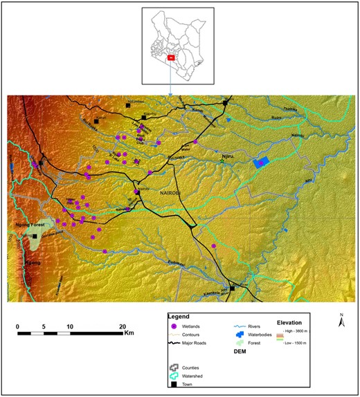
Location of Nairobi City County in the Kenyan context and a digital elevation model (DEM) map of the study area showing the location of the 31 wetlands.
Wetland sampling
Observing from Landsat satellite imagery of 2020, at an eye altitude of 400 m, there are ∼303 palustrine wetlands in Nairobi. The specification of the eye altitude was important as a key determinant of sample frame. This is because a lower or higher altitude would have led to identification of more or less wetlands respectively. This method of identification is unique because it allowed the inclusion of wetlands that Geographical Information Systems (GIS) processes would not reveal. Whereas GIS would only identify surfaces with water reflectivity, some of the palustrine wetlands are marshy, fully covered by hydrophytes, without water surfaces to reflect. Nevertheless, GIS analysis corroborated the presence of larger wetlands with open water, with blue colour assigned to water bodies.
Across the Nairobi city landscape, wetlands are found in natural depressions or are constructions. They may be marshy or boggy; with open water surface or completely covered by hydrophytes; or created for a variety of uses including recreational water features, agricultural dams, or sewage treatment plants. The wetlands may also be incidental, such as those created from abandoned quarries, or constructed such as those used for sewage treatment, and on private or public land.
A sample of 31 wetlands was drawn using the maximum variation sampling method. This involved delineating the city into blocks or districts (Lynch 1960; Jacobs 1961). This was to ensure that all areas of the city were represented. Secondly, from each city block, typical case sampling was used to select wetlands from each of the following categories: (a) the city blocks as bounded by major urban activity corridors e.g. Waiyaki Way and Thika Road main routes in Nairobi, (b) wetland origin e.g. whether constructed as a dam or are naturally occurring, (c) predominant land use context of wetland e.g. in an agricultural or residential area, and (d) predominant use of the wetland e.g. for sewage treatment or recreation. The proportions of the various categories are as shown on the pie charts in Supplementary Fig. S2.
Wetland configuration metrics
Wetland characteristics were observed using satellite images for the year 2020 and ground truthing conducted in the months of August and September 2020. Aspects of patch pattern such as area, perimeter, and edges were measured using Google Earth ProTM version 7.1 which has a positional accuracy of ≤ 1.8 m (Potere, 2008; Mohammed, Ghazi, and Mustafa 2013). This approach was found more reliable in accuracy for the identification of landscape elements surrounding the wetlands in greater detail. Additionally, it allowed for differentiation, identification, and estimation of proportions of the area of open water versus the area of hydrophytes. The wetland altitude was measured in the field using Garmin eTrex 10, 2.2 WAAS-enabled GPS hand held receiver.
The wetland configurational properties were categorized using landscape metrics classification techniques (McGarigal et al. 2012; With 2019). These techniques allow for the description of patterns at the patch, class or landscape scales. At the class level, wetlands were categorized into types differentiated by use of wetland, land-use context, and how the wetland was created. Table 1 shows the patch scale metrics used to measure wetland configurations in Nairobi.
Wetland patch-scale metrics.
| Metric | Code | Unit |
|---|---|---|
| Altitude/elevation | E | m |
| Area | A | ha |
| Perimeter | P | km |
| Core area | CA | ha |
| Perimeter of core area | PCA | km |
| Core area index | CAI | % |
| Perimeter/area ratio | P/A | – |
| Shape index | SI | – |
| Perimeter of wetland including 6 m edge | P6E | km |
| Area of wetland including 6 m edge | A6E | ha |
| Area of hydrophytes | AH | ha |
| Area of open water | AOW | ha |
| The perimeter of open water | POW | km |
| Area of open water index | IOW | – |
Figure 2 shows one of the wetlands sampled. It illustrates variability of wetlands in terms of shape, perimeter, and proportions of open water properties versus area covered by hydrophytes. More of these images are shown in Supplementary Fig. S3. A wetland core area excludes the outer edge, where in this study, the edge width was a buffer of 6 m. 6 m is the minimum width of a riparian buffer zone as per the Environmental Management and Coordination (Water Quality) Regulations 2006 (Government of Kenya 2006). Figure 3 illustrates measurements of wetland patch metrics using the ruler, polygon and buffering functions of Google earth ProTM. More of these images are shown in Supplementary Fig. S4.
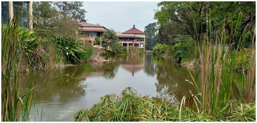
A storm water management pond at the Hub Shopping Mall, Karen which is ∼70% open water and 30% covered with hydrophytes.
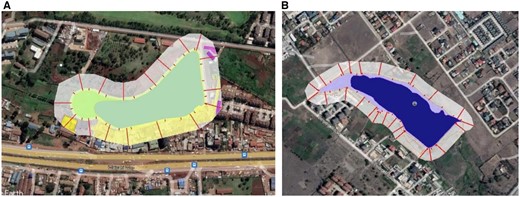
Google earth images showing the measurement of configurational properties of the wetlands: (A) Kangemi farm irrigation dam, and (B) Syokimau farm irrigation dam.
Aquatic macroinvertebrates metrics
Macroinvertebrates are exothermic animals without a backbone that are large enough to be seen with the naked eye. Some are terrestrial, while others are aquatic. Only aquatic macroinvertebrates were sampled including crayfish, leeches, odonates (including dragonflies), stoneflies, and beetles. Samples were collected from distinct wetland microhabitats, such as in pools, in macrophyte patches, under boulders, and in ground substrates. These samples were combined to form a composite sample per wetland. Some of the samples and collection processes are shown in Supplementary Fig. S5.
An area equivalent to 1 m2 was sampled for 15 min as per protocols suggested by Barbour et al. (1998). Sampling was done using 0.3 m width, 0.4 m length, and 0.3 m vertical height cuboid-shaped dip net of mesh size 0.5 µm. This was used as a kick net or for dipping, jabbing, and sweeping where appropriate.
Collected samples were preserved in 70% ethanol and taken to the laboratory for taxonomic identification. Laboratory identification was done using binocular microscope at Jomo Kenyatta University of Agriculture and Technology (JKUAT) Zoology Wet Laboratories. All specimens were identified morphologically to family level using available keys; thereafter marked and stored in the Zoology laboratory collections. Family taxon for macroinvertebrates is the basic unit used in water quality assessments (e.g. Gerber and Gabriel 2002; Tampo et al. 2021).
Shannon index is an important measure because it reveals two critical aspects of biodiversity structure. One is equitability in the biotic community in terms of the proportion of each family in the community. Secondly, it measures abundance—the number of individuals per family.
Statistical analysis
The data were analyzed using descriptive, correlational and inferential statistics. The mean, median, and mode, and measures of spread for the configurational metrics were calculated. Pearson Correlations (PCs) for predictive and response variables were evaluated to detect patterns of associations at the specific time of collection of samples from the given wetland cases. Multiple regression analysis was also done to test the hypothesis that wetland configuration significantly affects the biodiversity of AM of freshwater palustrine wetlands.
Before parametric analyses were done, the data were tested for normality. The Shapiro-Wilk test, read together with normal Q-Q plot, indicated that the number of macroinvertebrate families per wetland were normally distributed at W (31) = 0.94, P = 0.099. Data were analyzed using IBM Statistical Packages for the Social Sciences (SPSS) version 21. Pie charts, scatterplots, and box plots were used to present the data.
Results
Wetland patch scale configuration
Wetland patch characteristics varied significantly as per the descriptive statistics of configuration attributes (Table 2). There were wetlands with outlier values, mainly of the upper limit. For example, the Nairobi Sewage and Treatment Plant covers an area of 390.5 ha against an average of 3.0 ha. All outlier values were winzorised to within the fifth and 95th percentile to create more robust statistics for analysis (Sullivan, Warkentin, and Wallace 2021). The wetlands are distributed topographically within elevations (E) of 1494 m to 2000 m above sea level.
Descriptive statistics for wetland patch attributes.
| E (m) | P (km) | CA (ha) | A (ha) | P/A | SI | CAI (%) | P6M (km) | A6M (ha) | POW (km) | AOW (ha) | AHP (ha) | OWI | |
|---|---|---|---|---|---|---|---|---|---|---|---|---|---|
| Mean | 1770.4 | 0.958 | 2.92 | 3.53 | 3.74 | 1.30 | 79 | 1.00 | 0.660 | 0.780 | 1.45 | 1.77 | 0.627 |
| Median | 1803.0 | 0.780 | 1.88 | 2.49 | 3.31 | 1.25 | 80 | 0.760 | 0.500 | 0.610 | 0.605 | 1.41 | 0.656 |
| SD* | 112.3 | 0.588 | 2.38 | 2.74 | 1.93 | .245 | .121 | 0.648 | 0.419 | 0.630 | 1.65 | 1.44 | 0.498 |
| Range | 506.0 | 2.03 | 7.33 | 8.72 | 8.66 | .93 | 48 | 2.30 | 1.39 | 1.99 | 5.00 | 4.39 | 2.36 |
| Minimum | 1494.0 | 0.17 | 0.17 | 0.28 | 1.21 | 1.00 | 52 | 0.20 | 0.11 | 0.01 | 0.01 | 0.11 | 0.00 |
| Maximum | 2000.0 | 2.20 | 7.50 | 9.00 | 9.87 | 1.93 | 100 | 2.50 | 1.50 | 2.00 | 5.00 | 4.50 | 2.36 |
Patch shape complexity is measured by perimeter-to-area ratio (P/A) and patch shape index (SI) (With 2019). The wetlands exhibited varying shape complexity with P/A ranging from 1.21 and 9.87, and SI ranging from 1.00 and 1.93. The perimeter and area of the 6 m edge varied not only because of the size of the wetland but also because of the presence of islands and convolutions or straightness of the edges.
The minimum perimeter of open water (POW) was 0.01 km and a maximum of 14.96 km, while the area of open water (AOW) ranged from 0.01 ha to 362.01 ha. The area grown with hydrophytes ranged from 0.11 ha to 34 ha. Area of open water index was also calculated and it ranged from 0.00 to 2.36. Table 3 below shows all the values for wetland configuration attributes.
List of 31 wetlands, their use, and wetland configuration attribute values.
| Wetland | Wetland Use | E | P (km) | CA (ha) | P6e (km) | A (ha) | S/A | SI | CAI (%) | A6M (ha) | POW (km) | AOW (ha) | OWI | AH P | |
|---|---|---|---|---|---|---|---|---|---|---|---|---|---|---|---|
| 1 | Karura forest lily pond | Nature Conservation | 1685 | 0.6 | 1.2 | 0.6 | 1.9 | 3.3 | 1.1 | 0.6 | 0.7 | 0.4 | 0.5 | 0.4 | 1.4 |
| 2 | Karura forest butterfly marsh | Nature Conservation | 1715 | 0.7 | 2.7 | 0.7 | 3.0 | 2.4 | 1.1 | 0.9 | 0.3 | 0.0 | 0.0 | 0.0 | 3.0 |
| 3 | UON Kabete campus marsh | Agricultural Irrigation | 1832 | 0.6 | 1.7 | 0.6 | 2.5 | 2.6 | 1.0 | 0.7 | 0.8 | 0.2 | 0.1 | 0.1 | 2.4 |
| 4 | Kangemi dam | Domestic use | 1852 | 1.0 | 3.9 | 1.1 | 4.5 | 2.4 | 1.3 | 0.9 | 0.6 | 0.9 | 3.3 | 0.9 | 1.2 |
| 5 | Lakeview residential dam | Recreation | 1755 | 0.6 | 0.9 | 0.6 | 1.2 | 4.4 | 1.2 | 0.7 | 0.3 | 0.8 | 1.1 | 1.2 | 0.1 |
| 6 | Rosslyn Red Hill roadside marsh | Agricultural Irrigation | 1723 | 0.7 | 2.9 | 0.7 | 3.3 | 2.2 | 1.0 | 0.9 | 0.4 | 0.0 | 0.0 | 0.0 | 3.3 |
| 7 | Nyari residential estate dam | Recreation | 1718 | 1.2 | 4.1 | 1.2 | 4.7 | 2.5 | 1.4 | 0.9 | 0.7 | 1.2 | 4.1 | 1.0 | 0.7 |
| 8 | Evergreen Park dam | Recreation | 1700 | 0.7 | 1.6 | 0.7 | 2.0 | 3.5 | 1.2 | 0.8 | 0.4 | 0.7 | 1.6 | 1.0 | 0.4 |
| 9 | Paradise lost dam | Recreation | 1676 | 2.2 | 7.0 | 2.2 | 8.4 | 2.7 | 1.9 | 0.8 | 1.3 | 1.9 | 6.3 | 0.9 | 2.1 |
| 10 | Paradise gardens farm pond | Agricultural Irrigation | 1712 | 0.8 | 3.4 | 0.9 | 3.9 | 2.2 | 1.1 | 0.9 | 0.5 | 0.4 | 0.5 | 0.1 | 3.4 |
| 11 | Githurai quary pond | Abandoned Quarry | 1539 | 1.4 | 6.9 | 1.4 | 7.8 | 1.8 | 1.3 | 0.9 | 0.9 | 1.8 | 3.6 | 0.5 | 4.3 |
| 12 | Nairobi water sewage treatment plant, Ruai | Sewage Treatment | 1494 | 9.6 | 384.2 | 9.6 | 390.5 | 2.5 | 1.2 | 1.0 | 6.3 | 15.0 | 362.0 | 0.9 | 28.4 |
| 13 | Syokimau dam | Domestic use | 1607 | 1.4 | 5.8 | 1.4 | 6.7 | 2.1 | 1.3 | 0.9 | 0.9 | 1.1 | 4.6 | 0.8 | 2.1 |
| 14 | Nairobi dam, Kibera | Domestic use | 1688 | 4.1 | 31.3 | 4.2 | 34.0 | 1.2 | 1.8 | 0.9 | 2.7 | 0.3 | 0.2 | 0.0 | 33.8 |
| 15 | Ngong race course dam | Recreation | 1809 | 1.3 | 4.7 | 1.3 | 5.5 | 2.4 | 1.4 | 0.9 | 0.8 | 1.3 | 3.9 | 0.8 | 1.6 |
| 16 | Ngong road forest quarry pond | Abandoned Quarry | 1831 | 1.1 | 2.6 | 1.1 | 2.6 | 4.3 | 1.7 | 1.0 | 3.2 | 4.7 | 0.1 | 0.0 | 2.5 |
| 17 | Southern bypass roadside dam | Nature Conservation | 1844 | 0.6 | 0.8 | 0.7 | 1.2 | 5.6 | 1.5 | 0.7 | 0.4 | 0.4 | 0.5 | 0.7 | 0.6 |
| 18 | Southern bypass-Karen interchange dam | Nature Conservation | 1835 | 1.1 | 2.5 | 1.2 | 3.2 | 3.7 | 1.6 | 0.8 | 0.7 | 1.4 | 0.6 | 0.2 | 2.6 |
| 19 | Samburu Karen C, Hillcrest dam | Recreation | 1826 | 1.0 | 1.9 | 0.8 | 2.3 | 3.3 | 1.2 | 0.8 | 0.5 | 1.0 | 1.8 | 0.9 | 0.6 |
| 20 | Mamba Village dam | Recreation | 1806 | 0.8 | 1.5 | 0.8 | 2.0 | 3.9 | 1.4 | 0.8 | 0.5 | 0.8 | 1.5 | 1.0 | 0.5 |
| 21 | CUEA quary pond | Abandoned Quarry | 1798 | 0.2 | 0.2 | 0.3 | 0.4 | 7.0 | 1.1 | 0.6 | 0.2 | 0.2 | 0.2 | 0.7 | 0.2 |
| 22 | Karen country club sewage treatment plant | Sewage Treatment | 1856 | 0.7 | 1.9 | 0.8 | 2.3 | 3.3 | 1.3 | 0.8 | 0.5 | 0.0 | 0.0 | 0.0 | 2.3 |
| 23 | Langata botanical gardens pond | Recreation | 1803 | 0.2 | 0.2 | 0.2 | 0.3 | 7.1 | 1.0 | 0.6 | 0.1 | 0.3 | 0.2 | 2.4 | 0.1 |
| 24 | Karen roses greenhouses pond | Agricultural Irrigation | 1873 | 0.4 | 0.6 | 0.5 | 1.2 | 3.9 | 1.1 | 0.5 | 0.6 | 0.3 | 0.4 | 0.7 | 0.8 |
| 25 | Multimedia university sewage plant | Sewage Treatment | 1718 | 0.4 | 0.8 | 0.4 | 1.0 | 4.1 | 1.0 | 0.8 | 0.2 | 0.6 | 0.4 | 0.5 | 0.6 |
| 26 | The Hub Karen pond | Recreation | 1871 | 0.3 | 0.2 | 0.3 | 0.4 | 7.7 | 1.3 | 0.6 | 0.2 | 0.3 | 0.2 | 0.7 | 0.3 |
| 27 | Ondiri swamp, Maguga | Agricultural Irrigation | 1998 | 3.4 | 32.3 | 3.4 | 34.4 | 9.9 | 1.4 | 0.9 | 2.0 | 0.1 | 0.0 | 0.0 | 34.3 |
| 28 | Ondiri swamp, Gedion dam | Agricultural Irrigation | 2000 | 0.7 | 1.0 | 0.7 | 1.4 | 5.1 | 1.5 | 0.7 | 0.4 | 0.6 | 0.6 | 0.6 | 0.8 |
| 29 | Lenana high school dam | Agricultural Irrigation | 1821 | 1.4 | 4.4 | 1.4 | 5.3 | 2.7 | 1.5 | 0.8 | 0.8 | 1.8 | 2.5 | 0.6 | 2.8 |
| 30 | Mountain view estate marsh | Domestic Use | 1829 | 0.5 | 1.3 | 0.5 | 1.6 | 3.2 | 1.0 | 0.8 | 0.3 | 0.5 | 1.3 | 1.0 | 0.3 |
| 31 | Uhuru Park recreational pond | Recreation | 1671 | 0.8 | 1.7 | 0.7 | 2.2 | 3.3 | 1.2 | 0.8 | 0.5 | 1.1 | 1.4 | 0.8 | 0.8 |
Biodiversity of aquatic macroinvertebrates
Table 4 is a list of AM families per wetland, the family tolerance values, alpha and Shannon diversity. It also shows the total number of individuals per family and per wetland.
List of aquatic macroinvertebrate taxonomic order, families, common name, environmental sensitivity, alpha and Shannon diversity per wetland.
| No. | Class/Order | Family | Common name | Sensitivitya | Wetlands (31 No.) | TPFb | ||||||||||||||||||||||||||||||
|---|---|---|---|---|---|---|---|---|---|---|---|---|---|---|---|---|---|---|---|---|---|---|---|---|---|---|---|---|---|---|---|---|---|---|---|---|
| 1 | 2 | 3 | 4 | 5 | 6 | 7 | 8 | 9 | 10 | 11 | 12 | 13 | 14 | 15 | 16 | 17 | 18 | 19 | 20 | 21 | 22 | 23 | 24 | 25 | 26 | 27 | 28 | 29 | 30 | 31 | ||||||
| 1 | Coleoptera | Gyrinidae | Whirligig beetle | 4 | 14 | 0 | 4 | 23 | 0 | 6 | 0 | 0 | 8 | 0 | 0 | 48 | 0 | 16 | 0 | 3 | 2 | 11 | 0 | 18 | 0 | 0 | 0 | 0 | 7 | 14 | 8 | 0 | 0 | 0 | 1 | 183 |
| 2 | Coleoptera | Hydrophilidae | Hydrophilid beetle | 5 | 0 | 4 | 0 | 0 | 3 | 0 | 2 | 4 | 0 | 0 | 0 | 21 | 7 | 2 | 6 | 0 | 0 | 0 | 12 | 0 | 10 | 38 | 0 | 21 | 5 | 0 | 6 | 13 | 12 | 1 | 0 | 167 |
| 3 | Coleoptera | Hydrophilidae | Water scavenger beetle | 5 | 0 | 0 | 0 | 8 | 0 | 5 | 0 | 0 | 0 | 7 | 0 | 0 | 0 | 1 | 0 | 0 | 2 | 3 | 0 | 0 | 0 | 0 | 6 | 0 | 0 | 0 | 0 | 0 | 0 | 0 | 0 | 32 |
| 4 | Diptera | Chironomidae | Biting midge | 6 | 0 | 0 | 5 | 0 | 0 | 0 | 0 | 0 | 0 | 0 | 0 | 14 | 0 | 0 | 0 | 12 | 7 | 0 | 0 | 0 | 0 | 1 | 0 | 0 | 32 | 4 | 0 | 1 | 0 | 0 | 3 | 79 |
| 5 | Diptera | Chironomidae | Non-biting midge | 6 | 0 | 0 | 0 | 0 | 0 | 0 | 0 | 0 | 0 | 0 | 0 | 0 | 0 | 0 | 0 | 0 | 0 | 0 | 0 | 0 | 0 | 5 | 0 | 0 | 0 | 0 | 0 | 0 | 0 | 0 | 2 | 7 |
| 6 | Diptera | Simulidae | Blackfly | 7 | 0 | 0 | 0 | 0 | 0 | 0 | 0 | 0 | 0 | 0 | 0 | 0 | 0 | 0 | 0 | 0 | 0 | 2 | 7 | 0 | 0 | 0 | 0 | 0 | 0 | 0 | 0 | 0 | 0 | 0 | 0 | 9 |
| 7 | Diptera | Culicidae | Mosquito | 8 | 0 | 0 | 0 | 24 | 0 | 4 | 0 | 0 | 0 | 0 | 0 | 5 | 3 | 39 | 0 | 0 | 3 | 18 | 12 | 0 | 0 | 0 | 7 | 0 | 13 | 0 | 3 | 0 | 0 | 1 | 0 | 132 |
| 8 | Diptera | Tipulidae | Crane fly | 3 | 0 | 0 | 2 | 0 | 0 | 0 | 0 | 0 | 0 | 3 | 0 | 0 | 0 | 0 | 0 | 0 | 0 | 0 | 0 | 0 | 0 | 1 | 0 | 0 | 0 | 0 | 0 | 0 | 0 | 0 | 0 | 6 |
| 9 | Hemiptera | Geriidae | Pond water skater/strider | 6 | 0 | 0 | 0 | 13 | 0 | 0 | 0 | 0 | 0 | 32 | 0 | 0 | 5 | 0 | 0 | 9 | 2 | 5 | 0 | 2 | 0 | 1 | 0 | 0 | 0 | 10 | 6 | 0 | 0 | 0 | 0 | 85 |
| 10 | Hemiptera | Corixidae | Water boatman | 5 | 0 | 11 | 0 | 0 | 0 | 0 | 0 | 0 | 0 | 0 | 0 | 0 | 2 | 0 | 0 | 14 | 7 | 0 | 0 | 1 | 0 | 0 | 17 | 0 | 0 | 0 | 18 | 31 | 0 | 0 | 0 | 101 |
| 11 | Hemiptera | Mesoveliidae | Bugs (Aquatic) | 0 | 0 | 0 | 0 | 0 | 0 | 0 | 0 | 0 | 2 | 1 | 0 | 5 | 0 | 0 | 4 | 3 | 3 | 1 | 0 | 2 | 0 | 0 | 0 | 4 | 0 | 2 | 4 | 8 | 5 | 0 | 0 | 44 |
| 12 | Hymenoptera | Formicidae | Ant | 0 | 0 | 0 | 0 | 0 | 0 | 0 | 0 | 0 | 0 | 0 | 0 | 0 | 0 | 0 | 0 | 0 | 0 | 0 | 0 | 0 | 0 | 0 | 0 | 0 | 0 | 0 | 8 | 0 | 0 | 0 | 0 | 8 |
| 13 | Odonata | Chlorolestidae | Damselfly | 6 | 14 | 1 | 17 | 6 | 8 | 0 | 7 | 10 | 8 | 0 | 22 | 6 | 12 | 31 | 2 | 6 | 5 | 0 | 4 | 16 | 1 | 14 | 0 | 11 | 5 | 35 | 11 | 19 | 2 | 5 | 0 | 278 |
| 14 | Odonata | Aeshnidae | Dragonfly | 3 | 13 | 0 | 7 | 0 | 2 | 11 | 7 | 21 | 6 | 0 | 2 | 10 | 2 | 14 | 1 | 5 | 9 | 3 | 0 | 4 | 1 | 1 | 4 | 10 | 2 | 13 | 9 | 22 | 3 | 14 | 9 | 205 |
| 15 | Plecoptera | Perlidae | Stonefly | 1 | 0 | 0 | 0 | 0 | 0 | 0 | 0 | 0 | 0 | 0 | 0 | 0 | 0 | 0 | 0 | 1 | 0 | 0 | 0 | 1 | 0 | 0 | 0 | 0 | 0 | 0 | 0 | 0 | 0 | 0 | 0 | 2 |
| 16 | Trichoptera | Hydropsychidae | Caseless Caddisfly | 2 | 0 | 0 | 0 | 0 | 0 | 0 | 0 | 0 | 0 | 4 | 0 | 0 | 0 | 0 | 0 | 3 | 1 | 0 | 0 | 0 | 0 | 0 | 0 | 0 | 0 | 1 | 0 | 1 | 0 | 0 | 0 | 10 |
| 17 | Araneae | unidentified | Spider | 0 | 0 | 0 | 1 | 1 | 0 | 0 | 0 | 1 | 0 | 0 | 1 | 7 | 0 | 5 | 0 | 1 | 4 | 0 | 3 | 1 | 0 | 0 | 0 | 1 | 1 | 2 | 3 | 0 | 2 | 0 | 0 | 34 |
| 18 | Gastropoda | Planorbidae | Planorbid snail | 6 | 0 | 0 | 0 | 2 | 1 | 12 | 0 | 11 | 0 | 9 | 6 | 0 | 1 | 7 | 0 | 7 | 2 | 0 | 0 | 0 | 0 | 0 | 0 | 18 | 2 | 0 | 6 | 1 | 0 | 2 | 4 | 91 |
| 19 | Oligochaeta | Naididae | Sludge worm | 7 | 0 | 0 | 0 | 0 | 0 | 0 | 0 | 0 | 0 | 0 | 0 | 8 | 0 | 0 | 0 | 0 | 0 | 0 | 0 | 0 | 0 | 0 | 0 | 0 | 4 | 0 | 0 | 0 | 0 | 0 | 0 | 12 |
| 20 | Clitellata | Hirudinidae | Leech | 7 | 0 | 0 | 0 | 9 | 0 | 0 | 0 | 0 | 0 | 0 | 0 | 3 | 0 | 9 | 1 | 0 | 0 | 0 | 0 | 0 | 0 | 4 | 0 | 0 | 0 | 0 | 0 | 0 | 2 | 0 | 0 | 28 |
| 21 | Oligochaetae | Lumbricidae | Earthworm | 10 | 0 | 0 | 0 | 4 | 0 | 2 | 0 | 0 | 0 | 13 | 0 | 9 | 4 | 0 | 0 | 0 | 3 | 6 | 0 | 0 | 0 | 0 | 0 | 0 | 0 | 0 | 2 | 6 | 0 | 1 | 0 | 50 |
| 22 | Tricladida | Planariidae | Flatworm | 4 | 0 | 0 | 0 | 0 | 0 | 0 | 0 | 0 | 0 | 0 | 0 | 0 | 0 | 0 | 0 | 0 | 5 | 0 | 0 | 0 | 0 | 0 | 0 | 0 | 0 | 2 | 2 | 0 | 0 | 0 | 0 | 9 |
| 23 | Malacostraca | Decapoda | Cray Fish | 6 | 0 | 11 | 6 | 14 | 4 | 0 | 3 | 3 | 0 | 0 | 1 | 0 | 2 | 0 | 9 | 14 | 24 | 17 | 0 | 8 | 10 | 1 | 0 | 10 | 0 | 0 | 47 | 11 | 4 | 2 | 0 | 201 |
| 24 | Insecta | Megaloptera | 4 | 0 | 0 | 0 | 0 | 0 | 0 | 0 | 0 | 0 | 0 | 0 | 0 | 0 | 0 | 0 | 0 | 0 | 0 | 0 | 0 | 0 | 0 | 0 | 1 | 0 | 0 | 0 | 0 | 0 | 0 | 0 | 1 | |
| 25 | Diptera | Dixidae | Trueflies (dixed midge) | 1 | 0 | 0 | 0 | 0 | 0 | 0 | 0 | 0 | 0 | 5 | 0 | 0 | 0 | 0 | 0 | 0 | 0 | 0 | 0 | 0 | 0 | 1 | 1 | 0 | 0 | 0 | 0 | 0 | 0 | 0 | 0 | 7 |
| 26 | Hemiptera | Coreidae | 0 | 0 | 0 | 0 | 0 | 0 | 0 | 0 | 0 | 0 | 0 | 0 | 0 | 0 | 0 | 0 | 0 | 0 | 0 | 0 | 0 | 0 | 2 | 0 | 0 | 0 | 0 | 0 | 0 | 0 | 0 | 0 | 2 | |
| 27 | Ephemeroptera | unidentified | May fly | 1 | 0 | 0 | 0 | 0 | 0 | 0 | 0 | 0 | 0 | 0 | 0 | 0 | 0 | 0 | 0 | 11 | 4 | 0 | 0 | 0 | 0 | 1 | 0 | 0 | 0 | 1 | 6 | 1 | 0 | 0 | 0 | 24 |
| 28 | Hemiptera | Belastomatidae | Giant water bug | 0 | 0 | 0 | 0 | 4 | 0 | 0 | 0 | 0 | 5 | 0 | 0 | 0 | 0 | 8 | 0 | 1 | 0 | 0 | 0 | 0 | 0 | 0 | 1 | 0 | 0 | 8 | 10 | 14 | 0 | 0 | 0 | 51 |
| 29 | Insecta | Blattidae | Cockroach | 9 | 0 | 0 | 0 | 0 | 0 | 2 | 0 | 0 | 0 | 0 | 0 | 0 | 0 | 0 | 0 | 0 | 0 | 0 | 0 | 0 | 0 | 0 | 0 | 0 | 0 | 0 | 0 | 0 | 0 | 7 | 0 | 9 |
| TOTAL POPULATION | 41 | 27 | 42 | 108 | 18 | 42 | 19 | 50 | 29 | 74 | 32 | 136 | 38 | 132 | 23 | 90 | 83 | 66 | 38 | 53 | 22 | 70 | 36 | 76 | 71 | 92 | 149 | 128 | 30 | 33 | 19 | 1867 | ||||
| ALPHA DIVERSITY | 3 | 4 | 7 | 11 | 5 | 7 | 4 | 6 | 5 | 8 | 5 | 11 | 9 | 10 | 6 | 14 | 16 | 9 | 5 | 9 | 4 | 12 | 6 | 8 | 9 | 11 | 16 | 12 | 8 | 8 | 5 | |||||
| H’c |
| 1.14 | 1.67 |
|
| 1.75 | 1.26 | 1.47 | 1.99 | 1.68 | 0.96 |
| 1.94 |
| 1.51 | 2.37 | 2.42 | 1.87 | 1.48 | 1.68 | 0.99 | 1.53 | 1.41 | 1.78 |
| 1.87 |
|
| 1.71 | 1.64 | 1.37 | |||||
Sensitivity is the family tolerance value.
TPF is the Total Population per Family.
H’ is the Shannon Index of Biodiversity.
The total population count of the AM sampled was 1872 grouped in 29 families (Table 5). Two wetlands had the highest AM family richness of 16. One was the Ondiri swamp, H′ = 2.36. This swamp was the second largest wetland studied. The other was the Southern Bypass roadside dam, H′ = 2.42. The wetland with the second highest family richness of 14 was also located inside the Ngong Road Forest, H′ = 2.37, formerly a quarry for extracting murram, a gravelly lateritic material used for road surfacing in tropical Africa. This trend indicates that macroinvertebrates inhabit the less disturbed wetlands in natural areas such as forests and swamps.
Summary of aquatic macroinvertebrates biodiversity structure in the 31 wetlands.
| Population counts | Family richness | Abundant (population number) | Rare (population number) | Endangered | |
|---|---|---|---|---|---|
| Macro-invertebrates | 1872 | 29 | Chlorolestidae (Damsefly) (275) | Megaloptera (1) | Crayfish |
| Aeshnidae (Dragonfly) (205) | Coreidae (1) | ||||
| Decapoda (Crayfish) (201) | Perlidae (stonefly) (2) | ||||
| Gyrinidae (Whirligig beetle) (183) | Tipulidae (cranefly) (6) |
Two wetlands had only four families of AM, the lowest family richness (FR). One was the Nyari residential estate dam in a low-density residential area, H′ = 1.26. The other is the Catholic University of East Africa (CUEA) pond that was originally a stone quarry, H′ = 0.99. This wetland is located within an institutional context. It therefore means that where there are human settlements, the FR is relatively low.
In terms of abundance and rarity, it was found that the Chlorolestidae (Damselflies) with a population of 278, was the most abundant family, averagely distributed among the wetlands. The second and third most abundant family was the Aeshnidae (Dragonfly) and Decapoda (Crayfish) with a population of 205 and 201, respectively. The rarest families with a population of one or two were Megaloptera, Coreidae, and Perlidae (Stonefly). For bio-indication purposes, AM are classified in terms of their sensitivity to environmental pollution in a range of one to 10 (Hilsenhoff, 1988). A tolerance value of one represents the most sensitive aquatic macroinvertebrate family (AMF) to environmental pollution, and can only thrive in high quality water. The stonefly, mayfly, and the trueflies (dixed midges) are the most sensitive at tolerance value of one (Barbour et al. 1998; Ridl et al. 2018; Costa, Ferreira, and Pellegrini 2021). The tolerance value of 10 represent the most tolerant AMF that can live in highly polluted water such as those in Lumbricidae family–the earthworms. These results, therefore, indicate that most of the wetlands in Nairobi do not host a majority of the environmentally sensitive AM families because of high levels of water pollution.
The International Union for Conservation of Nature (IUCN, 2021) reports that 25% of freshwater grayfish species group are either critically endangered, endangered or vulnerable; while data is deficient for 21% of them. With a tolerance level of six, the crayfish family can thrive in relatively poor water quality environments. Although this family are the third most abundant in the Nairobi wetlands, this should not be construed as a sign of sustainability.
Table 6 shows the descriptive statistics of the alpha and Shannon index of diversity for the AM families. With a range of 13 AM families, there was high variation in habitability of the wetlands. This is because of the high variability in the wetland use, location and wetland configuration attributes including elevation and area. With a mean value of 1.685 for Shannon index of diversity H’, the Nairobi wetlands have a relatively high AMF biodiversity since the maximum H’ attainable in any habitat is up to 3.5 (Sweetlove 2011; Ortiz-Burgos 2016).
Descriptive statistics for alpha and Shannon index diversity of aquatic macroinvertebrates per wetland.
| Range | Minimum | Maximum | Mean | Std. Deviation | |
|---|---|---|---|---|---|
| Alpha diversity | 13.0 | 3.0 | 16.0 | 8.161 | 3.4746 |
| Shannon Index of diversity H’ | 1.46 | 0.96 | 2.42 | 1.685 | 0.38581 |
| Range | Minimum | Maximum | Mean | Std. Deviation | |
|---|---|---|---|---|---|
| Alpha diversity | 13.0 | 3.0 | 16.0 | 8.161 | 3.4746 |
| Shannon Index of diversity H’ | 1.46 | 0.96 | 2.42 | 1.685 | 0.38581 |
Correlations between wetland configuration and aquatic macroinvertebrates
Aquatic macroinvertebrates significantly and positively correlated with the wetlands shape index. This indicates that the more complex a wetland's shape, the higher the number of micro-habitats for macroinvertebrates to thrive. Likewise, the positive correlation between family richness and the perimeters P (km), PCA (km), together with area A6E (ha) further reinforces the observation that micro-habitats at the edges of wetlands are critical for this class of animals to persist in the city. Indeed, the edge effects created by the complexity of wetland shape and the long lengths of the wetlands are crucial planning and design considerations. On the contrary, attributes relating to the area of the wetland showed no significant association with the biodiversity of the macroinvertebrates. Table 7 shows the r values for these correlations.
Values of Pearson correlations (PC) r for wetland configuration variables and aquatic macroinvertebrates at the patch scale.
| Wetland Configuration | H' | E (m) | A (ha) | P (km) | CA (ha) | PCA (km) | CAI (%) | P/A | SI | A6E (ha) | P6E (km) | AH (ha) | AOW (ha) | POW (km) | IOW |
|---|---|---|---|---|---|---|---|---|---|---|---|---|---|---|---|
| Macroinvertebrates | 0.899** | 0.360* | – | 0.366* | – | 0.333* | – | 0.367* | 0.493** | 0.331* | – | – | – | – | – |
Correlation is significant at the 0.05 level (1-tailed).
Correlation is significant at the 0.01 level (1-tailed).
Regression analysis of wetland configuration and biodiversity of macroinvertebrates
The hypothesis that wetland configuration affects the biodiversity of macroinvertebrates in palustrine wetlands was tested using the F-test in multiple regression analysis of variance (ANOVA). To model the relationship between family richness and patch level wetland configuration, metrics of the core area index (CAI), shape index (SI), perimeter of wetland including 6 m wide edge (P6E), area of 6 m wide edge (A6E), open water area index (IOW), and elevation (E) were used.
Scatter plots were produced to visualize the relationships between FR and wetland patch configuration variables. Significantly, there is a strong positive relationship between FR and the complexity of the wetlands as measured by the shape index (Fig. 4). The relationship becomes even stronger when the wetlands are of smaller size of core area CA ≤ 2 ha.
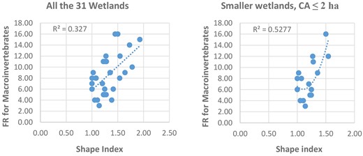
Scatter plots showing relationship between wetland shape index and macroinvertebrates family richness (FR).
Table 8 summarizes the multiple regression results. The regression model with all six predictors produced the model R2 = 0.587, F (6, 23) = 5.447, P < 0.001.
Summary of multiple regression results for macroinvertebrates at the patch scale.
| Model summary | |||||||||
|---|---|---|---|---|---|---|---|---|---|
| Model | R | R square | Adjusted R square | Std. error of the estimate | Change statistics | ||||
| R square change | F change | df1 | df2 | Sig. F change | |||||
| 1 | 0.766a | 0.587 | 0.479 | 2.60364 | 0.587 | 5.447 | 6 | 23 | 0.001 |
| ANOVAa—Macroinvertebrates | ||||||
|---|---|---|---|---|---|---|
| Model | Sum of Squares | df | Mean Square | F | Sig. | |
| 1 | Regression | 221.551 | 6 | 36.925 | 5.447 | .001b |
| Residual | 155.916 | 23 | 6.779 | |||
| Total | 377.467 | 29 | ||||
| ANOVAa—Macroinvertebrates | ||||||
|---|---|---|---|---|---|---|
| Model | Sum of Squares | df | Mean Square | F | Sig. | |
| 1 | Regression | 221.551 | 6 | 36.925 | 5.447 | .001b |
| Residual | 155.916 | 23 | 6.779 | |||
| Total | 377.467 | 29 | ||||
| Coefficientsa—Macroinvertebrates | ||||||
|---|---|---|---|---|---|---|
| Model | Unstandardized Coefficients | Standardized Coefficients | t | Sig. | ||
| B | Std. Error | Beta | ||||
| 1 | (Constant) | −28.811 | 15.375 | −1.874 | 0.074 | |
| Elevation in m | 0.020 | 0.006 | 0.562 | 3.582 | 0.002 | |
| Perimeter in m | 0.004 | 0.004 | 0.837 | 0.907 | 0.374 | |
| Shape Index | 2.320 | 3.112 | 0.160 | 0.745 | 0.464 | |
| Core Area Index | −2.452 | 8.571 | −0.080 | −0.286 | 0.777 | |
| Open water area index | −1.393 | 1.112 | −0.194 | −1.252 | 0.223 | |
Dependent variable: number of families of macroinvertebrates per wetland.
In the regression analysis, wetland altitude (E) was found to be of much significance in determining the distribution of macroinvertebrates P = 0.002. When simple regression analyses were performed separately between FR and SI, P6E, and P/A, they showed significant relationships at P = 0.005, P = 0.043, and P = 0.042 respectively.
Therefore, the explanation model for wetland configuration attributes was:
Aquatic Macroinvertebrates Y = -28.811 + (0.020 x Elevation) + (0.004 x Perimeter of wetland) + (2.320 x Shape Index)—(2.452 x Core Area Index)—(1.393x Open Water Index).
Further, the wetlands were grouped according to the criteria used during sampling. Analyses were carried out to assess patterns of association between AM families and the use of wetlands, the land use context. Box plots were used to represent the relationships between the AM and these classes of wetlands. Figure 5A indicate that there is a higher variety of up to 16 AM families that inhabit wetlands in forest land use contexts compared to 11 AM families that inhabit wetlands in commercial land use contexts. Figure 5B shows a corroboration of this finding where more AM families inhabit wetlands used for nature conservation, e.g. in forests. Wetlands used for sewage treatment understandably contained a lower variety of AM families.
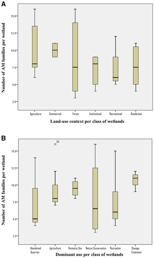
Box plots showing the relationship between aquatic macroinvertebrates and (A) the land-use context of wetlands, and (B) the dominant use of wetland.
Discussion
With growing urbanization, the loss of natural systems and their biodiversity, exacerbates already dire socio-economic situation for most urban residents, especially in the global south (Davoren & Shackleton 2021). Wetlands embedded in cities, together with urban forests, constitute the urban blue-green space systems that provide essential ecosystem services. The concepts, laws, methods, and principles of the emerging theory of urban ecology have been proposed to help mitigate on negative effects of urbanization on these systems (Pickett & Cadenasso 2017; Flies, Lim, and Douglas 2022). Successful mainstreaming of these systems in city planning will therefore be a robust way of building blue-green structural elements for improved human well-being in cities.
Characteristic of any water body, palustrine wetlands provide exclusive ecosystem services essentially because of the water-dependent biota in these systems. Wetland ecosystem services are important for the city socio-ecological sustenance (Ramsar Secretariat 2020; Xu et al. 2020), and especially for the urban poor (Palta, Grimm, and Groffman 2017). These services, whose foundational underpinning is biodiversity (MEA 2005; Hassall and Anderson 2015), include source of food and water, flood control; recreation; and aesthetics. The Nairobi landscape contains considerable amounts of natural and constructed wetlands. In addition, Nairobi is a city of many river systems (Supplementary Fig. S6) and its low-lying areas have historically been marshy savannah grasslands. Indeed the native Maasai community initially named Nairobi the place of cool waters (Akallah and Hård 2020). This study serves to highlight the importance of preservation of water in city planning and in the design of water infrastructure toward Nairobi wetland ecosystem restoration. This, correspondingly, is one of the goals of the United Nations (UN) declaration of the years 2021–2030 as the decade for ecosystem restoration (UN 2019; Dudley et al. 2020; Fischer et al. 2021; Jepson 2022; Nsikani et al. 2023).
Wetland configuration
This study adopted a fine-scale measurement of heterogeneity in form of wetland configuration. It was found that the wetlands are characterized by a variety of configurational attributes of area, perimeter and edge. The study sought to understand the relationship between wetland core area, area of open water, wetland perimeter, and the width of wetland edge on one hand; and the biodiversity structure of AM on the other. The area and perimeter of open water areas was particularly new and important way to understand wetland configuration, accounting for islands and hydrophytes. In Nairobi, wetland configuration is a function of wetland use and the process of creation of the wetland. For example, a wetland intended for sewage treatment would generally be regular in shape and with straight edges, resulting in a low shape index. Abandoned quarries that filled up with water, creating a wetland, were found to be highly irregular in shape, with convoluted edges, resulting in a higher shape index. Nairobi city has a high diversity of palustrine wetlands that are relatively distributed in the landscape. This diversity begets higher heterogeneity levels that beget higher biodiversity (Calcagno et al. 2017).
At the core of urban ecology is the integration of social and ecological systems so that human activities, as expressed in land uses, evolve together with variety of urban plants and animals (McDonnell and Niemelä 2011; Pickett et al. 2016). Urban wetland configuration, is therefore, one of the outcomes of human activities towards some urban function. The attributes of area, shape and edge were found to be critical determinants of heterogeneity, and consequently, the diversity of AM micro-habitats. Cortes et al. (2011) found that patch size and shape metrics of land uses affected benthic macroinvertebrate biodiversity in rivers. In urban rivers, landscape configuration at fine spatial resolution, explains more than 70% of the variability of instream macroinvertebrates (Huang and Gergel 2023). Although these studies were carried out in lotic systems, their findings are similar with those of this study.
In contrast with the generally accepted hypothesis that larger habitat patches have a higher level of biodiversity (Mittelbach and McGill 2019; Szangolies, Rohwäder, and Jeltsch 2022), this study found that there is no significant correlation between the distribution of AM with larger wetland area. The use of wetland played a more crucial role than wetland area. For example, the Nairobi water and sewage treatment plant was disproportionately larger than other wetlands but contained less diversity of macroinvertebrates. This may be attributed to the low quality of sewage water that affect biotic tolerance levels. It was also found that family richness of AM is positively associated with longer wetland perimeter and larger area of wetland edge. This is logical given the fact that a longer perimeter means more chances of AM microhabitats. These findings agree with the well-established generalization that there is positive correlation between complexity in perimeter and edge characteristics and species richness in patch habitats (Helzer and Jelinski 1999; McGarigal, Cushman, and Ene 2012; Xu et al. 2019).
For long, wetland conservation efforts have underscored on the creation of buffer zones with permanent vegetation (Graziano, Deguire, and Surasinghe 2022). In Kenya, up to 50 m wide buffer zone has been legislated as the distance required to protect a water body from irrigation activities (Government of Kenya 2006). However, a focus on buffer zone only is limiting, as compared to addressing conservation from landscape context perspective, and the development of scientific criteria for optimal buffer widths for wetland protection (Ma, 2016; Sawatzky and Fahrig 2019). This protection should be built on evaluation of catchment land use cover types and water quality analysis in multi time-space scale (Zhang, Liu, and Zhou 2018). In line with these efforts toward wetland conservation, this study presents new empirical knowledge of how wetland configuration affects the biodiversity of aquatic macroinvertebrates in urban wetlands. Therefore, there is need to rethink the criteria for conservation for existing and proposed wetlands.
Aquatic macroinvertebrates
Aquatic macroinvertebrates showed significant response to wetland configuration predictors. The variability of macroinvertebrate families could be explained up to 59% by wetland elevation, perimeter of wetland, shape index, core area index, and open water index at P = 0.001 significance level. These are important ecological statistics that city planning guidelines, processes and policy frameworks should consider so that these water-dependent biotic communities may be conserved.
Shape index was one of the most significant wetland attributes that explained the presence of AM in all the 31 wetlands at R2 = 33%. The coefficient of determination increases to R2 = 53% when the wetlands are smaller in area. This corroborates the findings that small patches are indeed vital for biodiversity conservation (Wintle et al. 2019). With a r = 0.493 for shape index, at a significance level of 0.001, this study provides evidence of how wetland shape complexity is a critical factor in the design optimization of urban wetlands towards increased wetland biodiversity.
Higher elevation within the watershed showed positive correlation with macroinvertebrate richness. This corresponds with the findings of Ao et al. (2022) who found that more species of macroinvertebrates inhabit high elevations of high mountain streams because of their functional traits e.g. swimming abilities. It therefore means that topographical elevation should be a factor to consider in planning so as to moderate on expectations of macroinvertebrate presence or absence.
Key drivers of declines in biodiversity of freshwater macroinvertebrates in tropical regions include water pollution, overexploitation, urbanization, habitat degradation and loss, hydrological alteration, climate change, population increase and invasive species (Rodríguez et al. 2012; Sundar et al. 2020). While this information is useful towards conservation efforts, this study has added to the conversation the need to consider wetland configuration as an important factor to manipulate in design for increased conservation. Despite 40% of world’s species inhabiting wetlands, these critical ecosystems are disappearing three times faster than forests (Convention on Wetlands 2021). AM are therefore a threatened class of animals specifically because of their complete dependence on wetland habitats for their feeding and breeding. This is particularly true for macroinvertebrate communities inhabiting urban wetlands in developing countries in Latin America, Africa, and Asia where the Convention on Wetlands (2018) report a decline in water quality since the 1990s.
With IUCN (2021) reporting declines on freshwater crayfish species, the statistics presented herein serve to highlight the crisis of biodiversity loss of AM. This is especially worse in urban areas or in landscapes with high human disturbance. Huang and Gergel (2023) observed that AM diversity decreases with increased level of urbanization. Human disturbance in watersheds impacts greatly on the composition and functional diversity of AM (Ao, et al. 2022). Regardless of the levels of urbanization, AM that are tolerant to pollution may dominate urban landscapes (Mackintosh, Davis, and Thompson 2015). However, there is great risk of the problem of increased cosmopolitan species, at the expense of native or endemic species, which effectively reduces and limits biodiversity. With menacing urbanization, it therefore demands of urban planning and design managers to institute processes that would guarantee conservation of macroinvertebrates, including the less tolerant groups in order to increase the species pool.
Out of the 29 AM families in Nairobi, 25% belong to the moderate to poor water quality tolerance ratings (Hilsenhoff 1987). It is only in two wetlands that the stonefly with a tolerance value of one was found. That is at the Mamba village, and the quarry wetland in Ngong Road Forest. These wetlands, which are located in the Karen area of Nairobi, indicate that the water quality in this neighbourhood is better than in other areas. This becomes the starting point for any AM conservation planning interventions to ensure that wetlands in the city are restored or protected from further pollution.
The desire to increase biodiversity in urban areas is well recognized (Parnell et al. 2013; Beatley 2016; Hill et al. 2017). Since AM play a crucial role in completing food chains and for ecosystem health, they therefore, become a key species group towards overall biodiversity conservation. Human well-being is the ultimate goal for increasing wetland biodiversity, and their indispensable ecosystem services (Xu et al. 2020). However, wetlands and their biodiversity are a common goods that suffer the tragedy of the commons (Hardin 1968). Whether in public or private land (Dyson et al. 2019), these common goods should be conserved because of their unique characteristics as urban patchy elements, ubiquitous distribution, and as biodiversity hotspots. Such conservation would result in a water-biodiversity city layer that would in turn entrench the love for wetland biota. Progressively, this idea would develop as a key concept in the planning and design of urban landscapes.
Conclusion
Although new urban wetlands are created, and existing ones are modified, the design concepts and processes applied hardly consider the need to increase diversity of aquatic macroinvertebrates. To increase and conserve aquatic macroinvertebrates in urban palustrine wetlands, area, perimeter, shape, and edge characteristics, as attributes of wetland configuration, should be planned and designed for. For example, the shape of the wetland should be convoluted to create more complex shapes with higher number of micro-habitats for macroinvertebrates. Wetland planning and design frameworks should be developed so that these ecological objectives are achieved without compromising on the function of the urban wetland. The frameworks should provide development control measures for the creation of new wetlands, and identification of existing and critical wetlands to be retrofitted, to foster wetland biological conservation and ecological stability.
Being the first research on wetlands at the city-wide scale, this study can provide baseline information for future monitoring and evaluation of wetland biodiversity trends in Nairobi and beyond. An analysis of trends of abundance or rarity of species and families of macroinvertebrates is one step towards their conservation efforts. Clarity of their geographical distribution, based on use of wetlands, the process of creation, and habitat preference would strengthen the mitigation of decline and loss of urban palustrine wetlands and their biodiversity.
Acknowledgements
We thank research assistants affiliated to the National Museums of Kenya (NMK) and the East Africa Nature Society (Nature Kenya). We thank David Ouma, Thomas Odeyo, Purity Njambi, Justus Ochong, Howard Atubwa, Mwadime Nyange and Peter Mureithi for assistance in field work data sampling, collection and processing. We also acknowledge the property owners in which the 31 wetlands are located, who granted access to the wetlands for this study.
Author contributions
Caleb Kiptum Toroitich(Conceptualization-Equal, Data curation-Equal, Formal analysis-Equal, Funding acquisition-Equal, Investigation-Equal, Methodology-Equal, Project administration-Equal, Resources-Equal, Software-Equal, Supervision-Supporting, Validation-Equal, Visualization-Equal, Writing—original draft-Lead, Writing—review & editing-Equal), Bernard Njuguna Mugwima(Conceptualization-Equal, Data curation-Equal, Formal analysis-Equal, Funding acquisition-Lead, Investigation-Equal, Methodology-Equal, Project administration-Equal, Resources-Equal, Software-Lead, Supervision-Lead, Validation-Lead, Visualization-Equal, Writing—original draft-Supporting, Writing—review & editing-Equal), and Dennis Kinyanjui Karanja(Conceptualization-Equal, Data curation-Equal, Formal analysis-Supporting, Funding acquisition-Supporting, Investigation-Equal, Methodology-Equal, Project administration-Equal, Resources-Equal, Software-Equal, Supervision-Equal, Validation-Equal, Visualization-Lead, Writing—original draft-Equal, Writing—review & editing-Lead)
Supplementary data
Supplementary data will be available at JUECOL online.
Funding
Funding was partially provided by the Jomo Kenyatta University of Agriculture and Technology (JKUAT). The field work was funded by the Africa-ai-Japan Project (JICA) based at JKUAT.
Conflict of interest statement
None declared.
Data availability
Data on wetland configuration are publicly available on Google Earth Pro. More data underlying this article are available in the article and in its online supplementary material.
