


Abstract
Asking people about their occupation is common practice in surveys and censuses around the world. The answers are typically recorded in textual form and subsequently assigned (coded) to categories, which have been defined in official occupational classifications. While this coding step is often done manually, substituting it with more automated workflows has been a longstanding goal, promising reduced data-processing costs and accelerated publication of key statistics. Although numerous researchers have developed different algorithms for automated occupation coding, the algorithms have rarely been compared with each other or tested on different data sets. We fill this gap by comparing some of the most promising algorithms found in the literature and testing them on five data sets from Germany. The first two algorithms we test exemplify a common practice in which answers are coded automatically according to a predefined list of job titles. Statistical learning algorithms—that is, regularized multinomial regression, tree boosting, or algorithms developed specifically for occupation coding (algorithms three to six)—can improve upon algorithms one and two, but only if a sufficient number of training observations from previous surveys is available. The best results are obtained by merging the list of job titles with coded answers from previous surveys before using this combined training data for statistical learning (algorithm 7). However, the differences between the algorithms are often small compared to the large variation found across different data sets, which we ascribe to systematic differences in the way the data were coded in the first place. Such differences complicate the application of statistical learning, which risks perpetuating questionable coding decisions from the training data to the future.
1. INTRODUCTION
Occupation coding—assigning verbal responses to an official occupational classification—has many faces. For example, people make implicit use of occupational coding algorithms when comparing their income online to that of other people in similar jobs (Tijdens, Zijl, Hughie-Williams, Kaveren, and Steinmetz 2010). In job recruitment, it is far easier to match job seekers with vacant positions if both are coded to the same occupational group (Bekkerman and Gavish 2011; Javed, Luo, McNair, Jacob, Zhao, et al. 2015). Prices for car insurance can differ depending on a customer’s occupational group (Scism 2016). Countless scientific studies, mainly in the fields of sociology, economics and epidemiology, include occupation in their statistical analyses. As the examples show, capturing individuals’ occupations is relevant in many fields.
The various applications are connected by a data collection process in which individuals are asked to describe their occupation, often using their own words, which are entered in a text field. For digital processing and analysis, it is then essential to categorize (code) the responses into systematic units; in this paper, the systematic units are the categories of the 2010 German Classification of Occupations (GCO) (Federal Employment Agency 2011). If thousands or even millions of answers have to be coded, the costs involved in employing human coders are substantial.
To save costs, high efficiency is essential. Since O’Reagon (1972) proposed an early algorithm for automated coding by computers, a substantial amount of research has been directed toward this goal (e.g., Klingemann and Schönbach 1984; Riviere 1997; Speizer and Buckley 1998). Yet, computers have rarely succeeded in replacing human coders completely and instead are often used to aid the coding process. One approach is to search for a given verbal answer in a coding index (the coding index used in this paper contains more than 50,000 job titles with their associated codes, e.g., “Mediadesigner → 23224”) and, upon finding a match, the algorithm selects the associated five-digit code, possibly to be double-checked by a human coder. This general approach—characterized by its reliance on a coding index—is in our experience often used in practice, though the specific implementations differ widely (e.g., Hartmann, Tschersich, and Schütz 2012; Elias, Birch, and Ellison 2014; Munz, Wenzig, and Bela 2016). By contrast, most recent research builds on ideas from statistical learning to predict the codes of new, incoming answers based on how similar answers were coded in the past. Many algorithms for occupation coding have been suggested in this diverse and disconnected literature (e.g., Creecy, Masand, Smith, and Waltz 1992; Measure 2014; Takahashi, Taki, Tanabe, and Li 2014; Russ, Ho, Colt, Armenti, Baris, et al. 2016; Gweon, Schonlau, Kaczmirek, Blohm, and Steiner 2017; Ikudo, Lane, Staudt, and Weinberg 2018) and a comparison of the different developments is urgently needed. We expect statistical learning algorithms to make occupation coding more efficient because they leverage previously collected training data from real studies and can perpetuate patterns found there, which is barely possible with expert-designed coding indexes.
Occupation coding can be viewed as a problem of automatic text classification (e.g., Sebastiani 2002; Grimmer and Stewart 2013; Gentzkow, Kelly, and Taddy 2019), but it entails some extra challenges. To begin with, the verbal answers about a person’s occupation are often short and can include misspellings. In addition, the classification problem is high-dimensional, with several hundreds of outcome categories and tens of thousands of distinct words uttered by respondents. On the one hand, this raises issues regarding the speed and efficiency of computation. On the other hand, the ideal training data would need to contain every possible input text more than once, requiring millions of observations, a number rarely collected in typical surveys. To alleviate this concern we pool data from multiple surveys. Moreover, manual occupation coding is not particularly standardized and coders frequently disagree about the correct category when coding identical answers (Elias 1997; Bound, Brown, and Mathiowetz 2001; Kim, Kim, and Ban 2019; Massing, Wasmer, Wolf, and Zuell 2019). No algorithm can code answers with high accuracy if humans do not agree about what is correct. We thus cannot expect to code every single answer automatically and without human control. However, we still see a possibility to partly overcome these challenges and achieve a larger degree of automation by employing better algorithms.
This article reviews and compares various algorithms for occupation coding, focusing on statistical learning algorithms. The algorithms under comparison have been carefully selected and several less-promising ones have been discarded. For the evaluation we adopt an applied perspective, asking how many answers could be coded automatically and how often the assigned categories would be identical with manual coding. Using the five data sets we have at our disposal, we showcase how much the results depend on the respective choice of training and test data. This allows us to identify the most competitive algorithms.
This research is part of our broader research agenda, which focuses on computer-assisted coding at the time of a survey interview (Schierholz, Gensicke, Tschersich, and Kreuter 2018). The idea is to present possible job categories directly to respondents, who can then choose the most appropriate occupation, thereby increasing data quality and reducing the workload for coders. Our research design and our analysis are influenced by this application. Other researchers may have their own application in mind or wish to replicate our analysis using their own data. For such purposes we provide a software package written in R (R Core Team 2018) at https://github.com/malsch/occupationCoding (last accessed July 30, 2020), which implements the various algorithms used in our research.
Section 2 reviews the major approaches that have been used to automate occupation coding and describes the rationale behind our selection of algorithms. Section 3 motivates the need to evaluate the performance in relative and absolute terms. Additional questions concern the use of multiple data sets. Section 4 provides key information about the data sets originating from six German surveys, their differences, and explains how we harmonized them. Section 5 describes the basic preprocessing steps required to make use of textual data, the mapping between research questions and data sets, and our approach to model tuning. Section 6 answers the research questions posed in Section 3. Section 7 concludes. Extensive Supplementary Material provides further details for each section and is available online.
2. ALGORITHMS
This article compares seven algorithms. They are selected either because they are frequently used in practice or because our literature review suggests they are most promising.
Coding index (exact matching) is our first algorithm. Many occupational classifications come with a coding index containing thousands of job titles and their associated codes (e.g., “Mediadesigner” → 23224), and their usage is straightforward. If the respondent mentions a job title that is included in the coding index, the corresponding code is assigned automatically. The coding index we use here is taken from the 2010 GCO (Federal Employment Agency 2011), which, after a few minor processing steps to aid matching, contains >25,000 male job titles (Mediadesigner) and another 25,000 female job titles (Mediadesignerin).
Despite this size, not every possible input text can be included in the coding index and exact matching will often fail. Respondents’ textual input and entries from the coding index may still be similar enough to be considered a match. This brings us to the second algorithm tested here, named coding index (similarity matching). This general approach—using a coding index and calculating similarities—is widely used and any comparison study would be incomplete without it. However, similarity calculations can differ in an infinite number of ways and best practices do not exist. One prominent computer program based on this approach is the “computer-assisted structural coding tool” (CASCOT) (Elias et al. 2014), which we use in the subsequent comparison. We load the same coding index as before into the program. To obtain better results, the developers recommend fine-tuning CASCOT by hand, essentially optimizing the way that similarities are calculated. We did not follow this advice but deliberately keep it simple to see how out-of-the-box solutions perform.
The algorithms described above were designed to utilize coding indexes, imitating their usage by professional coders. As an alternative, we next look at algorithms that were designed to learn prediction rules directly from previously coded answers, avoiding the need to construct a coding index by hand.
A shift toward statistical machine learning for occupation coding occurred when Creecy et al. (1992) published their algorithm, called memory-based reasoning. This algorithm contrasts with previous research conducted at the US Census Bureau, which was based on coding indices and similarity matching. Creecy et al. (1992) argued that their new algorithm outperformed the previous system by wide margins. Moreover, they developed the new system in just “four person-months while the [previous] expert system required 192 person-months.” The basic ingredient is a k-nearest neighbor algorithm based on two newly developed metrics, measuring the similarity between uncoded answers and previously coded ones.
In a similar vein, Gweon et al. (2017) proposed an adapted nearest neighbor algorithm for occupation coding. To classify a new response, the algorithm searches the training data for all responses that have the greatest cosine similarity (in a vector representation) and predicts the majority code among the training cases found (known as the 1-nearest neighbor algorithm). In addition to the predicted code, the adapted nearest neighbor algorithm outputs a confidence score, describing the likelihood of the predicted code being correct. The confidence score diminishes if the most similar responses were coded into several categories, if there are only a few most similar responses, or if the similarity of the most similar response is low. The authors compare their algorithm with linear kernel support vector machines, among others. The adapted nearest neighbor algorithm performed better than any competing algorithm.
The fifth algorithm in our comparison is multinomial logistic regression with elastic net penalization as implemented in the R-package glmnet (Friedman, Hastie, and Tibshirani 2010; Hastie, Tibshirani, and Wainwright 2015). The parameter matrix contains several million parameters in our application since both K, the number of distinct categories, and p, the number of unique words in the training data, are large. To deal with the high dimensionality, we employ elastic net regularization and shrink all parameters toward zero.
Linearity is a rather restrictive assumption of regression, as possible interactions between any two words are not taken into account. By contrast, tree-based methods can discover interactions automatically, promising better performance. The sixth algorithm, tree boosting (XGBoost), builds on the R-package XGBoost, which implements Friedman’s (2001) gradient boosting algorithm efficiently and has an impressive track-record in winning machine learning competitions (Chen and Guestrin 2016). The algorithm trains a sequence of decision trees iteratively, with each iteration focusing on training cases that the previous ones got wrong. The greater flexibility comes at a cost, however. There are a dozen tuning parameters in XGBoost, some of them relating to the overall gradient boosting algorithm, others relating to the algorithm that grows the individual trees, requiring a careful and time-consuming tuning step.
The seventh algorithm, tree boosting (XGBoost\w coding index) is almost the same as the sixth, the difference being that >50,000 job titles from the coding index (used with algorithms 1 and 2) are appended to the training data taken from surveys (used with algorithms 3–6). This makes it necessary to choose different tuning parameters as compared with the sixth algorithm.
Table 1 summarizes the key features of each algorithm. The Supplementary Material reviews related literature and describes the different algorithms in more detail.
Overview of Algorithms
| Algorithm | Reference data | Inferential technique | Outputa | |
|---|---|---|---|---|
| 1. | Coding index (exact) | Coding index | String identity | Code(s) (zero or more) |
| 2. | Coding index (\w similars) (CASCOT) | Coding index | String similarity | Code(s) (zero or more) \w confidence scores |
| 3. | Memory-based reasoning Creecy et al. (1992) | Previously coded | Bag-of-words and Vector similarity | Code (zero or one) \w confidence score |
| 4. | Adapted nearest neighbor Gweon et al. (2017) | Previously coded | Bag-of-words and Vector similarity | Code(s) (zero or more) \w confidence scores |
| 5. | Multinomial regression (glmnet) | Previously coded | Bag-of-words and Loss minimization | Codes (as in training data) \w predicted probabilities |
| 6. | Tree boosting (XGBoost) | Previously coded | Bag-of-words and Loss minimization | All codes from classification \w predicted probabilities |
| 7. | Tree boosting (XGBoost \w coding index) | Coding index and Previously coded | Bag-of-words and Loss minimization | All codes from classification \w predicted probabilities |
Probabilities have values between 0 and 1; in addition, the sum across all categories equals 1. This ensures that probabilities are comparable across different test cases, which is not the case for confidence scores.
3. RESEARCH QUESTIONS
Each algorithm has its own procedure to predict occupational categories for future data. To estimate the expected performance of each procedure, the predictions are compared with coded occupations from various test data sets.
We anticipate that some individuals will provide verbal answers that are difficult to code, for example, unforeseen new jobs and spellings, and any automatic procedure is almost certain to miscode them. If high data quality is desired, a human expert will need to code the most difficult cases, that is, those that the computer is likely to get wrong.
To acknowledge this, we look at two key metrics that are easy for practitioners to interpret. The production rate is the proportion of responses for which the automatic prediction procedure will be used. Since more automation reduces the amount of work for human coders, higher production rates can save coding costs. The agreement rate is the proportion of answers in which the top-ranked category from the algorithm and the “true” category from the evaluation data set are identical. Since “truth” is difficult to establish in occupation coding, a term like “accuracy” would be a misnomer. Instead, our term highlights whether automatic procedures are in agreement with current coding procedures. Ideally, we would like an agreement rate of 100 percent, implying that the automated coding procedure will always output the same categories as determined previously. However, the low rates of agreement between human coders raise doubt about whether human coding decisions are deterministic, a prerequisite for achieving perfect rates of agreement.
There is an inherent trade-off between the production rate and the agreement rate. If high production rates are desired, a larger number of hard-to-code answers need to be coded automatically, which are more likely to disagree. We expect decreasing agreement rates with increasing production rates.
Our first two research questions concern the performance of automated coding procedures in absolute and relative terms.
Question 1: For each algorithm, what is the trade-off between the agreement rate and the production rate?
Question 2: Which algorithm performs best?
Most of the algorithms described above need training data. Yet, creating training data requires expensive manual coding, which we wish to avoid. Instead, we use coded data from previous studies. A standard assumption in supervised learning is that training data and the future data to be predicted are drawn from the same distribution, resulting in identical patterns in both data sets. Since this assumption is probably not perfectly met when reusing data from previous studies, it is useful to know how robust the proposed algorithms are when using different training data. We compare the predictions based on different training data sets using the same test data set.
Question 3: How much does the agreement rate deteriorate if the training data and the test data have been created in different ways?
It is well recognized that supervised learning usually improves as the number of training observations increases. Especially for high-dimensional and local prediction problems, like occupation coding, we expect large gains because the ideal training data should contain several codings for every possible input text. Yet, few studies have coded more than 50,000 occupations in Germany. It is possible to increase the size of the training data if we pool data from various studies. This leads once again to concerns that studies may differ, contradicting the assumption that all observations are drawn from the same distribution. If the additional training observations are systematically different from those in the test data, the changed patterns in the training data would lead supervised learning astray and its agreement rate could deteriorate. The extent to which the performance can improve with more training observations is thus an empirical question.
Question 4: Can we improve predictions by pooling different data sets to increase the number of training observations?
The coding index used by algorithms 1 and 2 may be viewed as another source of training data besides survey data. Enriching the data from surveys with job titles obtained from a coding index may prove helpful, especially because a comprehensive coding index should contain codes for job titles that are uncommon in the general population and not necessarily available in the survey data.
Question 5: Can we improve predictions by enriching the training data with job titles from a coding index?
4. DATA
Our data stem from six different surveys. After pooling the data from two highly similar health-related studies, we have five data sets at our disposal. Specifically, our data are from the survey “Working and learning in a changing world” (data set A) (Antoni, Drasch, Kleinert, Matthes, Ruland, et al. 2010), the “BIBB/BAuA Employment Survey 2012” (data set B) (Rohrbach-Schmidt and Hall 2013), the “German Health Update 2014/2015” (Lange, Finger, Allen, Born, Hoebel, et al. 2017), the second wave of the “German Health Interview and Examination Survey for Children and Adolescents” (Hoffmann, Lange, Butschalowsky, Houben, Schmich, et al. 2018) (both pooled in data set C), the tenth wave of the panel study “Labour Market and Social Security” (data set D) (Trappmann, Beste, Bethmann, and Müller 2013), and the survey “Selectivity effects in address handling” (data set E) (Schierholz et al. 2018). Due to privacy concerns, verbal answers are generally not published along with these data sets. We describe all the data sets and their respective coding procedures in more detail in the online Supplementary Material.
The surveys differ to a considerable degree, and we highlight three such differences that might be most relevant with respect to our application. First, respondents were asked about different types of jobs, that is, about current jobs, past jobs, their parents’ jobs, and so on. Second, the question wording and its presentation in each study are often similar to one another, but not identical. Finally, the verbal answers in each study were coded by different coding agencies and, following Massing et al. (2019), we expect each agency to have their own coding conventions, implying that coding decisions will systematically differ if the same answers are coded by different agencies.
Table 2 provides a descriptive summary of the five data sets. The number of observations in each data set is calculated after excluding some verbal answers that we do not use in our analysis. The first reason for exclusion is if a verbal answer was coded into some category for “not employed.” This mostly happens if filters in the questionnaire were not used as intended and respondents answered occupational questions, although they should not have done so. These respondents did not report an occupation but something else (unemployed, retired, student, housewife, do not know, etc.). The second reason for exclusion is if answers are less than two characters long after the removal of punctuation marks and empty spaces and are therefore uncodable.
Data Summary
| (A) | (B) | (C) | (D) | (E) | |
|---|---|---|---|---|---|
| Mode | CATI | CATI | Paper and Web | CATI and CAPI | CATI |
| Coding agency | IAB | Kantar | RKI | infas | Kantar |
| First answer | |||||
| Number of job descriptions | 32,931 | 55,944 | 48,994 | 7,639 | 1,064 |
| Number of words | |||||
| Median | 1 | 1 | 1 | 2 | 1 |
| Mean | 1.6 | 1.6 | 1.8 | 2.9 | 2.1 |
| Maximum | 9 | 34 | 26 | 31 | 13 |
| Second answer (if informative) | |||||
| Number of job descriptions | 19,330 | – | 39,389 | – | 1,013 |
| Number of words | |||||
| Median | 2 | – | 5 | – | 5 |
| Mean | 2.7 | – | 5.5 | – | 6.7 |
| Maximum | 10 | – | 45 | – | 33 |
| Job codes | |||||
| Number of GCO codes useda | 853 | 1,057 | 1,106 | 685 | 351 |
| Frequency of special codes | |||||
| Student assistant | 308 | 60 | 124 | – | – |
| Volunteer/social service | – | 15 | 9 | – | – |
| Multiple jobs | 41 | – | – | – | – |
| Blue-collar worker | 50 | 797 | – | – | 1 |
| Not precise enough/uncodable | 152 | 1,805 | 311 | 186 | – |
The 2010 GCO consists of 1,286 five-digit job categories.
The amount of information available from each respondent, measured as the average number of words in each description, differs substantially between data sets. We believe that there are three main reasons for this: first, the questionnaire design differs in terms of positioning and the technical implementation of occupational questions; second, the interviewers may have different instructions concerning the level of detail needed; and third, the respondents may lack the motivation and ability to precisely describe a specific occupation they or their parents had a long time ago. All the respondents in data sets A, C, and E were asked a follow-up question to collect further details about their occupations. In contrast, the vast majority of respondents in data sets B and D were not asked a follow-up question.
Verbal answers in all data sets were coded according to the 2010 GCO (Federal Employment Agency 2011). Some occupations are very uncommon, so none of the studies used the complete range of 1,286 five-digit categories from the classification. Moreover, it is impossible to find one single appropriate category in the 2010 GCO for every verbal answer. To solve this problem, all the coding agencies introduced some additional, special codes that are not part of the official classification. Since we want to have codes that are comparable across data sets, we recode and harmonize the special codes. We retain only two extra categories for “Student assistant” and “Federal volunteer service/Voluntary social service/Civil service,” both arguably very job-like but not included in the 2010 GCO, and three broader, poorly defined categories “Multiple jobs,” “Job description not precise enough/Uncodable,” and “Blue-collar worker” for hard-to-code answers. Table 2 provides frequencies of the special codes in our data sets after harmonization.
5. ANALYTICAL STRATEGY
We would like to know how well each algorithm predicts categories from data set E and similar future data sets (questions 1 + 2). These test data were chosen because they represent our population of interest (adults were asked about their own occupation) and because more information than usual about each person’s job was available to coders, which we take as a sign of high data quality. Schierholz et al. (2018) analyzed the data quality in this data set. For these reasons, we have highest confidence in our evaluations when data set E is used. Results obtained from other data sets are a by-product of our analysis. They provide a robustness check and allow us to analyze whether particularities of the test data matter (question 3).
Making predictions is straightforward when the coding index is used (exact matching and CASCOT). In contrast, the choice of the training data matters for all other algorithms. To demonstrate this, we use data sets A, B, C, and D as training data and run separate analyses. In addition, we pool the four data sets to create a fifth data set, called (A, B, C, D). This last training data set allows us to analyze whether predictions improve when more training data from various studies are available (question 4).
The question as to whether the results improve when training data are enriched with job titles from a coding index (question 5) is investigated using algorithm 7 only. This algorithm is the same as algorithm 6, except that job titles from the coding index are added to the training data and the tuning parameters are adjusted.
To make verbal answers suitable for analysis, they are first standardized in a basic manner. Letters are lowercased and punctuation marks removed. Within most algorithms, we also replace special characters (e.g., “Ä” → “AE,” “€” → “EURO”) and trim space characters at the start and end of each string. We also considered stemming and removing stop words, but because we do not want to lose relevant information during data preparation, we regard these options as tuning parameters, to be tested in the model-tuning phase. After standardization, a document-term matrix (one row per answer, one column per word) is created from the answers, counting word frequencies for each answer. An additional column counting the total number of words in an answer can be appended to this matrix (tested with algorithms 5–7).
For all the algorithms that use training data, tuning parameters have to be selected that optimize the performance of the algorithms. Algorithms 3–5 have one or two method-specific tuning parameters each and a few additional parameters that control the transformation of text into a document-term matrix (see details in the Supplementary Material). Our general strategy here is to run a grid search over all reasonable parameter values, ignoring the less-promising ones, and to select the parameter configuration that performs best. Tree boosting (algorithms 6 and 7), however, has ten method-specific parameters that we wish to vary, implying that a full grid search over, say, 510 configurations (with five values per parameter) would take too long (20 minutes for a single run was not unusual). The final parameter configuration for tree boosting is therefore determined by means of analytic reasoning and empirical testing.
All data sets except E are split at random, resulting in 1,064 test observations for each (selected to be identical in size to data set E), and all the remaining observations are used as training observations. Since data set D is the smallest and the algorithms run fastest here, this data set is used to test and select possible tuning parameters. The same procedure (random splitting and grid search) is also tested on data set C to examine whether identical tuning parameters are still reasonable with this larger data set. The Supplementary Material contains complete results from the tuning process in both data sets and proves that a different choice of tuning parameters should not lead to substantial improvements.
As explained above, all the tuning parameters were selected using data sets D and C only, apart from two exceptions. The penalty parameter λ needed for logistic regression is dependent on the respective data set. Likewise, the number of iterations for boosting (and in algorithm 7 also γ) is dependent on the respective data set. As a result, evaluations using test data from data sets A, B, C, D and (A, B, C, D) need to be interpreted with caution since we glanced at these data sets to make the predictions. Nonetheless, we do not believe that this affects the results substantially—and data set E remained completely untouched.
.
Mathematical definitions of all the metrics used for evaluation are available in the Supplementary Material.
6. RESULTS
6.1 Preliminary Results
The simplest algorithm for automated coding is exact matching with a coding index (algorithm 1). Its results are shown in Table 3. The production rates vary between 28.7 and 48.8 percent. The production rate in data set D is low because many verbal answers are more than one word long—longer than usual job titles in the German language—making exact matching with job titles from the coding index all but impossible.
Production Rates and Agreement Rates from Coding with the Alphabetical Dictionary (Algorithm 1) for Each Data Set
| (A) | (B) | (C) | (D) | (E) | |
|---|---|---|---|---|---|
| Production rate (%) | 45.96 | 48.78 | 41.82 | 28.67 | 42.01 |
| Agreement rate (%) | 77.91 | 89.21 | 75.73 | 93.11 | 72.71 |
| (A) | (B) | (C) | (D) | (E) | |
|---|---|---|---|---|---|
| Production rate (%) | 45.96 | 48.78 | 41.82 | 28.67 | 42.01 |
| Agreement rate (%) | 77.91 | 89.21 | 75.73 | 93.11 | 72.71 |
Looking at the subset of answers that have matching entries in the coding index, the agreement rates between codes from the coding index and those from manual codings range between 72.7 and 93.1 percent. For comparison, Westermark, Franzen, and Kraft (2015) reported an ideal 100 percent agreement rate in a Swedish survey and Takahashi, Takamura, and Okumura (2005) were dissatisfied with agreement rates around 80 percent in Japanese surveys. Since our coding index can be understood as an “official” mapping of job titles into categories, implying that agreement rates should be 100 percent, the low agreement rates we find here may come as a surprise. However, coders may have reason to deviate from the coding index because if the first verbal answer is ambiguous, they may rely on other survey variables, for example, industry, supervisory status, occupational status, or the education usually required for a job. In addition, respondents were asked to describe their jobs in detail. Since the questionnaires and their implementation in the interviewing software differed, a second text field containing responses from all respondents is available only in data sets A, C, and E. If available, coders take this second text field into account when making their decisions, but the exact matching algorithm does not use this information. This second text field provides a plausible explanation for the lower agreement rates in data sets A, C, and E.
Exact matching with a coding index yields unsatisfactory results but provides a baseline for more advanced algorithms.
All the other algorithms are more flexible than exact matching as they output a confidence score (or a predicted probability) associated with the predicted category. We sort different verbal answers by this score. If the score is above a user-defined threshold, the textual input is coded automatically. This allows users to select their preferred production rate and its corresponding agreement rate.
Diagrams like the one in Figure 1 show the trade-off between production rates and agreement rates. They can also be used to compare the agreement rates of different algorithms at any fixed production rate. Although this type of visualization is our favorite way to compare the various algorithms, the space in this article is limited, forcing us to provide the complete set of diagrams only in the online Supplementary Material (Figures A2–A6). Some key results and important patterns from all the diagrams can also be seen in Table 4, which contains agreement rates when the production rates are fixed at 100 percent. However, this table neglects a key issue: if an algorithm does not achieve a 100 percent production rate, it will misclassify all remaining answers, resulting in a poor agreement rate at a 100 percent production rate even if the same algorithm excelled at lower production rates.
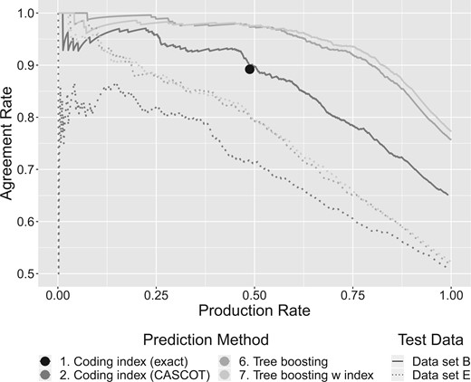
Agreement Rates of the Most Probable Category at Various Production Rates. Example: 48.8 percent (production rate) of the responses in test data set B have an exact match with the coding index (algorithm 1). Within this subset, 89.2 percent (agreement rate) of the assigned categories agree with evaluation data. The production rates and their respective agreement rates of any other algorithm are controlled by the user choosing a threshold.
Agreement Rate (%) at 100 Percent Production Rate ± Standard Errors
| Training data | |||||
|---|---|---|---|---|---|
| (A) | (B) | (C) | (D) | (A, B, C, D) | |
| Test data are from the same data set as the training data | |||||
| 1. Coding index (exact) | 35.81 ± 1.47 | 43.52 ± 1.52 | 31.67 ± 1.43 | 26.69 ± 1.36 | 35.06 ± 1.46 |
| 2. Coding index (CASCOT) | 56.58 ± 1.52 | 64.57 ± 1.47 | 52.82 ± 1.53 | 55.64 ± 1.52 | 57.05 ± 1.52 |
| 3. Memory-based reasoning | 67.95 ± 1.43 | 73.50 ± 1.35 | 58.18 ± 1.51 | 57.61 ± 1.51 | 64.47 ± 1.47 |
| 4. Adapted nearest neighbor | 65.60 ± 1.46 | 74.15 ± 1.34 | 57.05 ± 1.52 | 57.52 ± 1.52 | 63.82 ± 1.47 |
| 5. Multinomial regression | 68.14 ± 1.43 | 76.41 ± 1.30 | 59.02 ± 1.51 | 60.34 ± 1.50 | 58.93 ± 1.51a |
| 6. Tree boosting (XGBoost) | 66.92 ± 1.44 | 75.66 ± 1.32 | 59.68 ± 1.50 | 59.12 ± 1.51 | 63.82 ± 1.47 |
| 7. Tree boosting (\w cod index) | 68.14 ± 1.43 | 77.26 ± 1.29 | 61.18 ± 1.49 | 63.35 ± 1.48 | 69.08 ± 1.42 |
| Test data are from data set E | |||||
| 1. Coding index (exact) | 30.55 ± 1.41 | 30.55 ± 1.41 | 30.55 ± 1.41 | 30.55 ± 1.41 | 30.55 ± 1.41 |
| 2. Coding index (CASCOT) | 50.66 ± 1.53 | 50.66 ± 1.53 | 50.66 ± 1.53 | 50.66 ± 1.53 | 50.66 ± 1.53 |
| 3. Memory-based reasoning | 43.52 ± 1.52 | 49.62 ± 1.53 | 47.84 ± 1.53 | 39.10 ± 1.50 | 53.95 ± 1.53 |
| 4. Adapted nearest neighbor | 42.86 ± 1.52 | 49.34 ± 1.53 | 45.77 ± 1.53 | 38.16 ± 1.49 | 53.29 ± 1.53 |
| 5. Multinomial regression | 45.02 ± 1.53 | 51.50 ± 1.53 | 49.72 ± 1.53 | 40.23 ± 1.50 | 49.25 ± 1.53a |
| 6. Tree boosting (XGBoost) | 44.17 ± 1.52 | 51.69 ± 1.53 | 49.15 ± 1.53 | 39.85 ± 1.50 | 54.70 ± 1.53 |
| 7. Tree boosting (\w cod index) | 47.56 ± 1.53 | 52.26 ± 1.53 | 50.56 ± 1.53 | 49.06 ± 1.53 | 56.20 ± 1.52 |
Regularized multinomial regression does not converge in data sets (A, B, C, D), leading to poor performance.The best-performing algorithms are highlighted (bold) for each data set.
6.2 Question 1: For Each Algorithm, What Is the Trade-Off between the Agreement Rate and the Production Rate?
We first look at the results obtained when the training data are from data set A, B, C or D, and the test data are from the same data set (upper left in Table 4). Since the table is limited to agreement rates at a 100 percent production rate, we consult diagrams from the Supplementary Material for complementary results at lower production rates.
The performance of the algorithms varies widely between different data sets. For example, at a 100 percent production rate tree boosting (algorithm 6) achieves a 59.1 percent agreement rate in data set D and 75.7 percent in data set B. At a 50 percent production rate, it achieves an 88.9 percent agreement rate in data set D and 97.4 percent in data set B. The absolute performance thus depends on the specific data set in use. Generalizations for new data sets are hard to obtain.
6.3 Question 2: Which Algorithm Performs Best?
Looking at the production rates achieved by the exact matching algorithm, Figures A2–A5 in the Supplementary Material show that in each data set exact matching (algorithm 1) and CASCOT (algorithm 2) exhibit similar agreement rates if the production rates are fixed by algorithm 1. Yet, as a major improvement, the CASCOT algorithm provides greater flexibility, allowing users to choose any production rate they like. If a 100 percent production rate is desired, the differences between the two algorithms are more pronounced (see Table 4), reflecting that this metric, the agreement rate at a 100 percent production rate, is ill-suited to describe the performance of the exact matching algorithm.
Table 4 and Figures A2–A5 in the Supplementary Material show that all the other algorithms outperform the CASCOT algorithm, sometimes by wide margins of more than ten percentage points. Only memory-based reasoning (algorithm 3) is usually worse at low production rates.
Comparing the four algorithms that rely on training data only (algorithms 3–6) with each other, the agreement rates at a 100 percent production rate are quite similar within each data set (see Table 4). The differences between the worst-performing and the best-performing algorithm are usually small, never exceeding three percentage points. These small differences may well be irrelevant to a practitioner. If we still wish to rank the different algorithms by their relative performance in each data set, penalized multinomial regression is often best. XGBoost is a close competitor on all data sets. Memory-based reasoning and the adapted nearest neighbor algorithm oftencome in third and fourth places.
This changes if we examine agreement rates at low and medium production rates (see Figures A2–A5 in the Supplementary Material). All the algorithms outperform memory-based reasoning by wide margins. Similarly, but only at very low production rates, the agreement rates from penalized multinomial regression are poor. Memory-based reasoning and penalized multinomial regression are overconfident and output scores that are too high for answers that are in fact difficult to code. Only XGBoost and the adapted nearest neighbor algorithm achieve agreement rates that are close to optimal at low and medium production rates.
Tree boosting (with coding index, algorithm 7) tends to perform better than all the other algorithms discussed so far (see question 5 below).
6.4 Question 3: How Much Does the Agreement Rate Deteriorate If the Training Data and the Test Data Have Been Created in Different Ways?
The data set that best represents our future application is data set E. Respondents in this data set were asked several questions about their own job to facilitate high-quality manual coding. The results obtained from this data set are therefore of particular interest.
If data set E is used for evaluation and not data from the same data set that was used for training (see lower panel of Table 4), the agreement rates drop dramatically, in some cases by >25 percentage points. It appears that the automatic coding of data set E is particularly hard: the exact matching algorithm and the CASCOT algorithm (algorithms 1 and 2) perform least well on data set E (see Figures A2–A5 in the Supplementary Material), even though neither of the algorithms relies on training data. A possible explanation is that we used only the first verbal answer for automatic coding, whereas human coders had access to additional information.
The relative performance of the algorithms in data set E is very similar to the results described above. In particular, at a 100 percent production rate, multinomial regression and XGBoost (algorithms 5 and 6) are better than both the memory-based reasoning and the adapted nearest neighbor algorithms (algorithms 3 and 4). In contrast to what was reported previously, the CASCOT algorithm (algorithm 2) becomes a competitive algorithm if tested on data set E. Its agreement rate at a 100 percent production rate is higher than those from any other algorithm trained on one of the data sets A, C or D.
6.5 Question 4: Can We Improve Predictions by Pooling Different Data Sets to Increase the Number of Training Observations?
Data sets A, B, C, and D are pooled to form a combined data set (A, B, C, D), which is then split at random to obtain 144,444 training observations and 1,064 test observations. We also note that the size of the training data sets differs. Data set D is the smallest, with 6,575 training observations; data set A has 31,867 training observations; data set C contains 47,930 training observations; and data set B has 54,880 training observations.
The last column of Table 4 shows the agreement rates for the pooled data set and Figure A6 in the Supplementary Material shows results at lower production rates. All the algorithms using training data (algorithms 3–7) perform better in data set E as the number of training observations increases [D < A < C < B < (A, B, C, D)]. An exception is multinomial regression, which did not converge.
However, the improvements are not as large as expected. Even though our largest data set (A, B, C, D) is more than three times larger than data set C, the agreement rate at a 100 percent production rate in test data E improves by just a few percentage points and remains below 57 percent. Other strategies would be needed for more substantial improvements.
6.6 Question 5: Can We Improve Predictions by Enriching the Training Data with Job Titles from a Coding Index?
In algorithm 7, job titles from a coding index were added to the training data and the tree boosting algorithm was retrained. The additional information from the coding index improves the predictions as can be seen by comparing algorithms 6 and 7. This effect is most pronounced with training data set D, probably because relatively few patterns are encoded within this small data set, allowing the algorithm to find the largest number of additional patterns in the coding index.
The highest agreement rates for data set E are achieved after pooling all the available training data and adding information from the coding index. This highlights the usefulness of having a large training data set for automated occupation coding.
7. DISCUSSION
Manual occupation coding is time-consuming, and its automation has been a longstanding goal. We compare different algorithms for this purpose and find that the common practice of using algorithms that rely on job titles from a coding index (algorithms 1 and 2) can be improved by using statistical learning algorithms (algorithms 3–7) that rely on training data from previous surveys. The more training observations are available, the better the results, although we had hoped for more substantial improvements. The performance of the algorithms can be improved further if training data from surveys are enriched with job titles from a coding index (algorithm 7). Multinomial regression with elastic net penalization and tree boosting (algorithms 5 and 6) tend to outperform techniques that were designed specifically for occupation coding (algorithms 3 and 4) at a 100 percent production rate, although the differences are small and may not matter in practice. Since training the adapted nearest neighbor algorithm (algorithm 4) is faster, this algorithm might still be preferred to find out quickly which performance is achievable.
The performance of any algorithm strongly depends on the data set used. For example, half of the answers from test data set B could be coded completely automatically with near perfect agreement. By contrast, in data sets C and E, the agreement rate (at a 50 percent production rate) is rarely above 80 percent. We put these differences down to the different ways that the data sets were created. High agreement rates are found in data sets A and B, which made extensive use of an exact matching algorithm for its creation, enforcing a high degree of standardization (= two identical verbal answers found in the coding index are given identical codes). In data sets C, D, and E, for which we find lower agreement rates, coders presumably based their decisions on additional information provided by respondents (not used by our algorithms), leading to less standardization (two identical verbal answers might be assigned to different categories due to the additional information). These (and possibly other) data-related factors explain much of the variation between our performance measures, more than the choice of algorithm.
Agreement rates around 80 percent may not suffice for high-quality coding. How can machine learning still be leveraged if no algorithm performs well enough for fully automated coding? One option is computer-assisted coding (Campanelli, Thomson, Moon, and Staples 1997; Bushnell 1998; Speizer and Buckley 1998). In this setting an algorithm suggests a short list of possible categories, assisting human coders with their decisions. Existing software tools for computer-assisted coding are typically based on a coding index and similarity matching (e.g., algorithm 2). Our results indicate, however, that algorithms based on statistical learning can generate better category suggestions and could be used instead, but only if sufficient training data are available.
A limitation in this study is that we use verbal answers from a first open-ended question only. Other information, which is often used for manual coding (e.g., texts from a second open-ended question, occupational status, industry), was not used in this paper. Clearly, the algorithms should improve if they were to use the same information that professional coders have used for their decisions. We did not consider any additional information because such information will not be available for the application we have in mind. The idea is to suggest possible categories to the respondents at the time of the interview and to let them choose the most appropriate job category themselves (Tijdens 2015; Schierholz et al. 2018). This should happen without asking other coding-related questions, which would prolong the interview.
This article tests seven algorithms for occupation coding and compares their performance. We show that certain statistical learning algorithms can achieve superior performance and may be worth implementing in practice. The specifics will always depend on the planned application (fully automated coding, computer-assisted coding or interview coding) and on the available training data. Data scientists may wish to explore the possibilities open to them with their own data. To facilitate this, we make our code available in an R-package, downloadable at https://github.com/malsch/occupationCoding (last accessed: 07/30/2020).
Supplementary Materials
Supplementary materials are available online at academic.oup.com/jssam.
Malte Schierholz prepared this paper as part of his PhD thesis.
This work was supported by the German Institute for Employment Research; the Mannheim Centre for European Social Research; and the German Research Foundation (KR 2211/3-1). Matthias Schonlau’s research was supported by the Social Sciences and Humanities Research Council of Canada (SSHRC # 435-2013-0128). We are grateful for the support provided by the Federal Institute for Vocational Education and Training (BIBB) and the Robert Koch Institute (RKI), who made available two of the five data sets used in this study. We sincerely thank our colleagues at the German Institute for Employment Research and the University of Mannheim for their valuable comments.
References
Federal Employment Agency (
R Core Team (
