


Abstract
Weather-related risk makes the insurance industry inevitably concerned with climate and climate change. Buildings hit by pluvial flooding is a key manifestation of this risk, giving rise to compensations for the induced physical damages and business interruptions. In this work, we establish a nationwide, building-specific risk score for water damage associated with pluvial flooding in Norway. We fit a generalised additive model that relates the number of water damages to a wide range of explanatory variables that can be categorised into building attributes, climatological variables, and topographical characteristics. The model assigns a risk score to every location in Norway, based on local topography and climate, which is not only useful for insurance companies but also for city planning. Combining our model with an ensemble of climate projections allows us to project the (spatially varying) impacts of climate change on the risk of pluvial flooding towards the middle and end of the 21st century.
1 Introduction
A recent report by the World Meteorological Organization found that floods were the most common of weather-, climate-, and water-related disaster types recorded in the period 1970–2019 (Douris et al., 2021). While single events of large fluvial (river) floods can cause damages worth billions of Euros (Barredo, 2007), a large proportion of overall flood damages is caused by pluvial flooding—surface water flooding resulting from heavy rainfall—due to the far greater reach of these events (Houston et al., 2011; Spekkers et al., 2011). For instance, Houston et al. (2011) assess that around 2 million people in the UK are at risk from pluvial flooding. Pluvial floods are commonly considered an invisible hazard, as they can strike with little warning in areas with no recent record of flooding (Netzel et al., 2021), and the risk of pluvial flooding may increase in the future due to a combination of climate change, urbanisation and lack of investment in sewer and drainage infrastructure (Skougaard Kaspersen et al., 2017).
A building’s exposure to pluvial flood risk depends on a range of factors such as the building’s attributes, local weather, and topography. The extent to which these factors influence the risk exposure is commonly assessed based on insurance claims data on reported flood damages, see Gradeci et al. (2019) for a systematic review of the use of insurance claims data in analysing pluvial flood events. A critical challenge when assessing flood impact is the lack of good quality flood impact data (Hammond et al., 2015). One specific challenge is that insurance claims data may not separate between fluvial and pluvial flood damage (Bernet et al., 2017). In Norway, however, fluvial flood damage is covered by a compulsory natural perils insurance linked to fire insurance and managed by the Norwegian Natural Perils Pool, while pluvial flood and other rainfall-induced damage is covered by a private insurance and managed directly by the primary insurer. In the following, we do not separate between pluvial flood and other rainfall-induced damage, and, for simplicity, we refer to these as water damages.
The study of water damage and its relationship to meteorological, hydrological and topographical variables is nicely summarised in Lyubchich et al. (2019), and Gradeci et al. (2019). A commonality among these studies is that the number of claims and the claim size is aggregated in space [see Table 6 in Gradeci et al. (2019) and Table 3 in Lyubchich et al. (2019)], for example at the level of municipality or postal code. Many papers also model daily claim frequency or severity and use meteorological and hydrological variables that are associated with the specific daily event, see for example Spekkers et al. (2014) and Haug et al. (2011). For assessing the risk of specific buildings, or risk on an annual basis (for example, for pricing) there are two drawbacks of using a daily model on spatially aggregated data. Firstly, spatially aggregated data disguise building-specific information, which makes it hard to assess the risk of a specific building at a specific location. Variables such as topographical indices that are available at a high spatial resolution will also lose their accuracy and thus potentially explanatory power if spatially aggregated. A second challenge of a daily model that uses daily weather variables is that predicting future claims beyond approximately two weeks is challenging due to the high uncertainty of possible weather outcomes and a lack of skilful long-range weather predictions for this time resolution (van Straaten et al., 2020).
The goal of this study is twofold. Our first goal is to provide an estimation of current, or near-term, water damage risk for any building or potential building site in Norway. Our second goal is to project potential changes in water damage risk in a future climate. To this aim, we employ detailed topographical information at a m resolution over Norway and a more general quarterly summary of local weather statistics as detailed information of future weather is unlikely to be robustly projected for a future climate. Insurance data from the insurance company Gjensidige, including information on building attributes—to account for building-specific risk—and reported water damages are available for 729,031 unique locations in Norway within the time period 2009–2021. These data cover approximately a quarter of the national market. The output of our analysis is the risk of water damages for a property located anywhere in Norway. Here, we compare the use of a generalised additive model with either a Poisson or a negative binomial likelihood. The parametric structure of the models is such that the individual risk components related to topography, weather, and building characteristics can be extracted and assessed individually or combined.
2 Data
Our model incorporates several different data sets. Claims data from the insurance company Gjensidige are combined with topography data derived from a digital elevation model (DEM) and historical meteorological data provided by the Norwegian Meteorological Institute. Moreover, regional climate projections provided by the EURO-CORDEX initiative are used to project claim frequency for future climate scenarios. A brief description of these data sets follows.
2.1 Insurance data
The insurance data were provided by the Norwegian insurance company Gjensidige and contain customer information from 1 January 2009 to 23 April 2021. The data set contains insurance information for private houses, apartments, cabins, agricultural, and industrial buildings, as well as apartment complexes with a single coverage for the entire complex, located in Norway. For each insured property, we have information on the exact location, the insurance period, the value of the property, whether the building is used as a rental property and building characteristics such as size, age, type of roof and whether the building has a basement. In our analysis every building with its unique combination of characteristics constitute one observation. Modification of any property attribute, e.g. its size, over the building’s insurance period gives rise to separate observations with associated coverage lengths. The data set includes 32,534 water damage claims, corrsponding to an average of 0.007 claims per insured year. Overall, the buildings in the data set have between 0 and 15 claims. Out of observations, (99.5%) contain zero claims.
2.2 Topography data
Topographical information is obtained from the Norwegian Mapping Authority’s DEM corresponding to the bare-Earth surface where all natural and built features are removed. The DEM is generated from data primarily collected via airborne laser-scanning equipment and organises 10 m gridded elevation data into non-overlapping 50 km square blocks. Rather than constructing one huge national data set, we assemble blocks into regional rectangles of manageable size, where each region typically covers 1–3 counties (there are a total of 11 counties in Norway). The rectangular area is chosen large enough so that it encompasses the full hydrological catchment area for every single location within any of the counties that it represents. To further facilitate processing of the regional DEM data, a coarser spatial resolution of 20 m is established by averaging the elevation of the four 10 m cells underlying every 20 m cell.
From the 20 m gridded and regionalised DEM data, three topographical indices of particular interest to precipitation-induced damage are calculated: Height Above Nearest Drainage (HAND) (Nobre et al., 2011), which specifies for each grid cell in the DEM the relative elevation between the cell and the nearest waterway cell (for example, river or ocean) that it drains into. One interpretation of the HAND index is that it judges the risk of a DEM cell being affected if its associated waterway overruns its banks. The second index is the slope, β, of a DEM cell which specifies the local angle of inclination in the water flow direction out of the cell and measures the capability that a grid cell has to drain water away. A similar concept that also takes into account the amount of water potentially flowing into the DEM cell is the Topographical Wetness Index (TWI) developed by Beven and Kirkby (1979). This is defined as , where a is the size of the upslope contributing area and β is the slope. Grid cells with a high TWI therefore indicate locally flat terrain or a large upslope area, both of which increase the likelihood of accumulating water.
2.3 Meteorological data
Historical meteorological information is derived from the gridded data product seNorge version 2018 (Lussana, 2020). Using statistical interpolation of station observations, seNorge contains estimates of daily near-surface air temperature and precipitation on a grid with resolution 1 km covering all of Norway from 1957 to the present day. The seNorge data set is used to derive climatological indices on the same resolution, defined as quarterly means of daily temperature and precipitation for the time period 1991–2020. In addition to these climatological indices, several alternative climatological indices were considered in an explorative stage of our research. This included high empirical quantiles of the quarterly distributions of daily temperature, daily precipitation, and multi-day precipitation as well as high return period values from intensity–duration–frequency curves for daily precipitation. However, as these did not improve the predictive performance of our models and yielded less interpretable models, we have chosen to focus on the quarterly means of precipitation and temperature, which are more robust climatological indices.
2.4 Climate projections
Projections of the climatological indices for a future climate are provided by the EURO-CORDEX initiative (Jacob et al., 2020). EURO-CORDEX provides a multi-model ensemble of regional climate projections for Europe at a spatial resolution of 12 km, obtained by running a limited-area regional climate model (RCM) using the output of a global general circulation model (GCM) as boundary conditions. In addition, the RCM output has been bias-corrected using a cumulative distribution function transformation (Michelangeli et al., 2009; Vrac et al., 2012) or distribution-based scaling (Yang et al., 2010), using data from the regional reanalysis MESAN (Häggmark et al., 2000; Landelius et al., 2016) or the observation-based gridded data product E-OBS (Cornes et al., 2018) as calibration data.
Specifically, we consider 12 different combinations of GCMs, RCMs, and bias-correction approaches, as listed in Table 1. This multi-model ensemble of climate projections includes two different GCMs (EC-EARTH Hazeleger et al., 2012 and MPI-ESM-LR Giorgetta et al., 2013), four different RCMs (CCLM4-8-17, HIRHAM5, RACMO22E, and RCA4, see Jacob et al., 2014 for details), as well as three different versions of the bias-correction approaches described above. Considering such a variety of combinations helps us better account for the uncertainties associated with each layer of modelling. Additionally, we consider two representative carbon pathways (RCPs): RCP 4.5 is an intermediate scenario where emissions peak around 2040 and decline afterwards, while RCP 8.5 presents a worst-case scenario where emissions continue to rise throughout the entire 21st century (Jacob et al., 2014).
Overview of the EURO-CORDEX climate projection ensemble used in this paper
| GCM | RCM | Bias-correction method | |
|---|---|---|---|
| 1 | EC-EARTH | CCLM4-8-17 | CDFT22s-MESAN-1989–2005 |
| 2 | EC-EARTH | CCLM4-8-17 | DBS45-MESAN-1989–2010 |
| 3 | EC-EARTH | HIRHAM5 | CDFT22s-MESAN-1989–2005 |
| 4 | EC-EARTH | HIRHAM5 | DBS45-MESAN-1989–2010 |
| 5 | EC-EARTH | HIRHAM5 | CDFt-EOBS10-1971–2005 |
| 6 | EC-EARTH | RACMO22E | CDFT22s-MESAN-1989–2005 |
| 7 | EC-EARTH | RACMO22E | CDFt-EOBS10-1971–2005 |
| 8 | EC-EARTH | RCA4 | DBS45-MESAN-1989–2010 |
| 9 | MPI-ESM-LR | CCLM4-8-17 | CDFT22s-MESAN-1989–2005 |
| 10 | MPI-ESM-LR | CCLM4-8-17 | DBS45-MESAN-1989–2010 |
| 11 | MPI-ESM-LR | RCA4 | CDFT22s-MESAN-1989–2005 |
| 12 | MPI-ESM-LR | RCA4 | DBS45-MESAN-1989–2010 |
Note. For each ensemble member, the general circulation model (GCM), the regional climate model (RCM), and the bias-correction method (combination of method, data product, and data period) is listed.
An ensemble of future climatological indices for two future periods, 2031–2060 and 2071–2100, are obtained by calculating the projected differences of the climatological index between the future period and the historical period 1991–2020 from each climate model. These projected differences are then added to the historical index, derived from the seNorge data. Considering differences rather than absolute projections removes potential (constant) biases of the climate models. The projected future indices are therefore derived on the high-resolution spatial scale of 1 km provided by seNorge, but for all grid cells lying within the same km RCM grid cell the same changes apply.
3 Methods
3.1 Statistical modelling framework
The aim of the statistical modelling is to predict the number of claims, , for contract i. To this aim, we model the distribution of as a function of various covariates and use the length of the contract, , as offset. Our covariates can be grouped in four separate classes: (1) property-specific characteristics, (2) topographical information at the property location, (3) climatological information at the property location, and (4) a fixed effect of which county the property is located in and a random effect over municipalities to increase the flexibility of the model. This way, municipalities with little information get regularised towards the mean of the county, which is important since many municipalities contain only few observations. Currently, there are 11 counties and 356 municipalities in Norway.
For the climatological indices, we compare annual models based on annual averages of precipitation and surface temperature to quarterly models based on quarterly averages. For the latter, each contract i is split into (up to) four sub-contracts. For example, a contract from 1 January 2019 to 20 January 2020 would be split into four contracts, accounting for the respective overlaps: a contract of 3 months and 20 days in quarter 1 (Q1), and three contracts of 3 months each in Q2–Q4. The claims of the original contract are then assigned to the sub-contracts of the appropriate quarter. This increases the temporal resolution of the climate statistics, enabling the model to pick up on quarterly differences in claims connected to seasonal differences in weather. Note that we estimate a single model over all quarters. That is, we assume the same effect of the climate statistics throughout the year, only their value may vary by season.
For the distribution of , we compare a Poisson and a negative binomial model, denoted by and , respectively. For both distributions, is the expected number of claims for the ith contract. While the distribution of the Poisson model is fully determined by its mean, the negative binomial model has an additional parameter θ, specified by . In particular, the negative binomial model exhibits larger variance than the Poisson model, and the parameter θ controls for overdispersion.
For both models we employ a generalised additive model (GAM; Hastie & Tibshirani, 1990). This allows for non-linear relationships between the covariates and the number of claims without needing to specify the functional form of these relationships, while still being highly interpretable. The interpretability aspect is crucial for understanding and explaining the risk structure to both potential insurance holders and decision-makers in the context of climate change adaptation. We use a logarithmic link function, such that the relationship between the expected number of claims and the available covariates is specified by
Here, represents the vector of categorical variables for contract i with parameter vector and represents a smooth function modelling the effect of the jth continuous covariate . The variable is a random effect assigned to each policy i belonging to municipality with in the current setting as one municipality has no weather data available. The variables and represent the length of the ith contract and the value of the building, respectively, which are used as offsets in our model. The final model contains five discrete and continuous covariates. The discrete variables include a fixed effect for the county and are otherwise property specific, e.g. whether a property has a basement and the quality of the building. The continuous variables include climatological, topographical, and property-specific covariates, see Section 4.1 for details.
We assume that the effects, , for all municipalities are independent and normally distributed with a common variance , that is, . Normally distributed random effects fit nicely into the GAM framework, as they can be expressed as a smooth spline with a penalty matrix equal the identity matrix. They can therefore be estimated simultaneously with the smooth splines in equation (1) (Wood, 2017). The offset accounts for the increase in expected claims over time as long as the contract is active. The use of the property value, as offset is convenient in insurance risk modelling, where it is more natural to model the number of claims per time and insured value, which is more closely connected to the expected payout. Since it would be unreasonable to assume to increase linearly in , we additionally consider as a property-specific covariate.
Each is represented as a weighted sum of basis functions,
where the are unknown parameters to be estimated from the data, and are known basis functions, here given by the truncated thin plate regression basis (Wood, 2003). It should be noted that, specifically for precipitation, a natural alternative to the truncated thin plate basis would be a spline basis that enforces monotonicity, see Meyer (2018). This would ensure that the risk of water damage increases in the precipitation amount. This methodology has been investigated using the package cgam (Liao & Meyer, 2019), but is too computationally demanding given the size of our data and does, moreover, not support the negative binomial distribution.
3.2 Risk assessment
We define the risk of the ith contract as , that is, the expected number of claims per year and value of insured property. The structure of the GAM facilitates that the risk can be decomposed into the product of partial risks corresponding to different groups of covariates. For example, the non-standardised climatological risk for the ith contract is defined as
where the sum runs over the climatological covariates only (i.e. average precipitation and surface temperature). The partial climatological risk is then obtained by standardisation
where the average in the denominator is taken with respect to all contracts. This standardisation achieves that the average climatological risk equals 1, making it easy to see whether a given contract has above- or below-average risk due to local climatology. Similarly, we can define the partial topographical risk and the partial building-specific risk , by restricting the right-hand side of equation (1) to only the summands corresponding to covariates of these groups. The covariates not belonging to either of these three groups are the county fixed effect and the municipiality random effect, which we group into the partial regional risk . This yields a complete decomposition of the total risk of the ith contract as
This decomposition facilitates interpretation of the results. The factor is the same for all contracts and, therefore, represents base risk. Each of the four other factors averages to 1, making it easy to identify prevailing risk drivers (or risk reductors) for a specific property. The decomposition also allows visualisation of spatially varying risk, by plotting maps of the partial risks, see Section 4.2. Note that, after fitting a model, these risk factors can be calculated for all locations for which the corresponding covariate information is available yielding national risk maps.
3.3 Inference
In order to avoid overfitting, we employ a penalised log-likelihood given by
where is the log-likelihood, are the model parameters, are the smoothing parameters controlling the smoothness of the s and the precision () of the random effect, and is a matrix where the klth element equals . The model parameters and smoothing parameters are estimated in two steps. First, equation (3) is optimised w.r.t holding fixed using penalised iteratively reweighted least square (PIRLS). Second, the smoothing parameters are estimated using Laplace approximated restricted maximum likelihood, holding fixed. For the negative binomial model, the dispersion parameter θ is estimated alongside the smoothing parameters.
All computations are performed with R version 4.0.5 (R Core Team, 2021) using the package mgcv version 1.8-26 (Wood, 2011) for parameter estimation of the GAMs. As our data set contains millions of observations and hundreds of covariates (when all levels are one-hot encoded), we use the methodology proposed for large data sets in Wood et al. (2017), Wood et al. (2014), and Li and Wood (2020), as implemented in the bam function in mgcv.
3.4 Model evaluation
We evaluate and compare competing models using two proper scoring rules (Gneiting & Raftery, 2007), the mean square error (MSE) and the Brier score (Brier, 1950), where a smaller value equals a better performance.
The MSE is defined as
where is the observed number of claims for the ith contract, is the length of the contract (in years), and is the predicted expected number of claims for . The scaling factor counteracts the fact that the variance of grows with the length of the contract. It can be shown that under this scaling, the rank of competing models is equal for different time units in the contract length.
The distribution of the claims data is heavily skewed. While for the vast majority of contracts we have , the data also contains many contracts with two or more claims, some contracts even reaching more than 10 claims. The MSE is sensitive to such outliers (Thorarinsdottir & Schuhen, 2018), and an evaluation using the MSE therefore puts specific emphasis on the predictive performance for these outliers. To complement the picture, we therefore consider the Brier score as a second performance metric. Specifically, we consider the mean Brier score for the event of observing at least one claim,
where denotes the indicator function and is the predicted probability that the ith contract files at least one claim. This metric is insensitive to outliers and shifts the focus to predicting whether a given house will have a claim or not.
3.5 Model selection methodology
For assessing out-of-sample predictive performance, we perform a 10-fold cross-validation where 10% of the contracts are removed at random during model fitting, and the fitted model is used to predict the claims for the withheld 10%. This process is repeated 10 times with each contract left out exactly once during the model training.
We compare using either a Poisson or a negative binomial target distribution for the regression model as well as four alternative configurations of the regression model in equation (1). The simplest baseline model includes only building-specific covariates. Additionally, we consider a model including topographical indices (TWI, slope, and HAND), a model including climatological indices (mean temperature and mean precipitation) and a model including both topographical and climatological indices.
For the climatological information, we consider both a quarterly and an annual model as discussed in Section 3.1 above. The splitting into quarterly sub-contracts results in a different set of contracts than for an annual model, which makes it difficult to directly compare the MSE and the Brier score for these models. We address this by reversing the quarterly split before evaluation. Specifically, for the quarterly model, the ith contract is split into (up to) four contracts during fitting, with corresponding numbers of claims . After fitting the model, we obtain four different predicted means . For evaluation, we recompute and consider this quantity a prediction for . Similarly, for the Brier score we obtain four probabilities and can retrieve as , assuming conditional independence of the number of claims across different quarters.
Under the Poisson model, the sum of the four quarterly predictions is again Poisson distributed. The only difference is that the quarterly model resolves seasonal variation in the climatological indices. However, for the negative binomial model, a change in model resolution yields a different model distribution (Diggle & Milne, 1983), so that the annualised quarterly model is not directly comparable to the annual model.
3.6 Model diagnostic
After selecting a model as described above, we assess the fit of the final model using conditional expectation diagrams. Such diagrams are obtained by sorting the prediction–observation pairs by their predicted expectation , and thereafter dividing into k sub-groups of equal size. The conditional expectation diagram then plots a single point for each group, its x-coordinate being the mean predicted expectation, or mean , for the group and its y-coordinate being the mean conditional expectation, or mean , for the group. Since the predictions were sorted before grouping, the predicted expectation gradually increases in the group index from 1 to k. For example, the point with the highest x-value corresponds to the group of highest predicted risks. For a perfectly calibrated prediction model, the k points are located on or near the diagonal. Systematic deviations from the diagonal reveal conditional biases of the predictive model, see Section 4.1 for details. These diagrams constitute a straightforward generalisation of reliability diagrams which are widely used as a diagnostic tool for prediction of categorical variables, see Wilks (2011).
4 Results
Here, we present the results of our analysis of Norwegian water damage data. In a cross-validation study, we compare risk assessment models with different sets of covariates at two temporal resolutions and under two different distributional assumptions. We then present estimates of annual water damage risk under current and future climate.
4.1 Model selection
Figure 1 shows the out-of-sample predictive performance of 16 different risk assessment models based on a cross-validation study, where the models differ in distributional assumptions, covariate selection, and temporal resolution. A baseline model that only includes property-specific information is outperformed by models that include topographical and/or climatological variables. Further, as expected, including topographical information with high spatial precision gives a greater improvement in performance than including more general climatological information. Concerning model distribution, we see clear improvement in performance for the negative binomial model if the estimation is performed at a quarterly temporal resolution, even for the baseline model where all the covariates are identical. In the negative binomial model, the mean and the θ parameter are estimated jointly, and there is a non-linear relationship between the mean and the variance. If the estimation is performed at a quarterly time resolution, the variance of the resulting annualised model tends to be smaller than that of the original annual model. This, in turn, affects the mean estimate and leads to slightly larger annual mean estimates, in particular for contracts with large expected number of claims. Consequently, the predictive errors are smaller for these contracts yielding an overall smaller MSE.
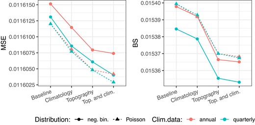
Comparison of models for water damage risk in Norway under a Poisson and a negative binomial likelihood with property-specific covariates only (baseline), additional climatological or topographical information, or both. Annual risk is estimated based on four quarterly models, or a single annual model. We assess predicted number of annual damage claims using MSE (left) and predicted probability of seeing one or more claims per year using the Brier score (right). Scores are given as mean scores over a 10-fold cross-validation of the entire data set.
While proper scoring rules favour the true data generating process by construction, they may evaluate different aspects of competing models and thus not always yield identical rankings when none of the models represent the true data generating process. The best performance of each distributional model is obtained when both topographical and climatological information is included in the model. However, the model rankings for this setting are not consistent across the two types of evaluation in Figure 1. The quarterly Poisson model ranks first under MSE and third under the Brier score, while the quarterly negative binomial model ranks second under MSE and first under the Brier score. As the overall highest ranked model, we continue our analysis with the negative binomial model estimated on a quarterly basis with both topographical and climatological covariates.
Risk models for the insurance industry are often perceived as not performing particularly well at predicting high numbers of claims, see Scheel et al. (2013) for an example. In our case, out of the 6 million contracts, 99.5% have zero claims and 138 contracts have between 3 and 7 claims. The mean predicted number of claims for these extreme observations is 0.192, due to many observations with similar covariate values having zero claims. While this is substantially higher than the overall mean of 0.005, it nevertheless seems like a gross underestimation. For the most extreme observation with 7 claims the model predicts a chance of just under 0.05% of observing 7 or more claims, and similarly small probabilities are achieved for almost all observations with 3 or more claims. Unintuitively, however, this does not indicate a bad predictive fit in the context of the full data set. In fact, out of 6 million observed contracts, roughly 3000 contracts should fall above the 99.95th percentile of their predictive distribution. This highlights the importance of perceiving the predictions as probabilistic, rather than expecting the mean of the prediction to be always close to the observed number of contracts.
In order to avoid this fallacy associated with evaluating predictive performance of a model based on only the most extreme observations (Lerch et al., 2017), we consider conditional expectation diagrams. Figure 2 shows out-of-sample conditional expectation diagrams for this model. Here, we consider the contracts on the quarterly time resolution, which results in roughly 6 million contracts. The left diagram considers sub-groups with 60,000 values in each. We observe an overall very good fit of the model. The right diagram considers only the 100,000 contracts with the highest predicted number of claims. That is, it considers the contracts approximately corresponding to the two rightmost points in the left diagram. The diagrams show that, even for the high-risk customers, the model is well calibrated and does not exhibit conditional bias. The shown diagrams are constructed from the cross-validation results and therefore assess the model fit out-of-sample, as is appropriate for our prediction setting.
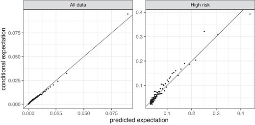
Conditional expectation diagrams for the quarterly negative binomial model using both topographic and climatological covariates. The right-hand side diagram is constructed from the 100,000 contracts with the highest predicted number of claims .
Figure 3 shows the estimated effect of the topographical and climatological covariates for the quarterly negative binomial model. Specifically, we show the multiplicative effect of these variables by taking the exponential of the additive effect. All response panels share the same scale for the y-axis, but the range is suppressed to prevent adaptation of the fitted model by direct competitors of Gjensidige. The top row shows the effect of the three topographical indices. The TWI has a clear linear effect. The higher the wetness index the higher the expected number of claims. The effect of the slope index is shaped as a parabola with a minimum at approximately 10 degrees and a higher risk for both a lower and a higher slope. The effect of the slope index is difficult to interpret independently of the TWI which directly depends on the slope. The estimated spline for slope having a clearly pronounced shape gives evidence that information is added by considering both variables. The HAND index has the largest effect when its value is between 0 and 100 m. This is intuitive since, at a certain point, it becomes irrelevant to move even higher above the nearest drainage point. The effect of precipitation is clearly non-linear; for low values the effect is flat, then close to linear between 3 and 9 mm of average daily precipitation in a quarter. The decreasing effect for precipitation values above 9 mm is somewhat counterintuitive and might be the result of little data in the upper tail, or signal a localised adaptation to current climate in very wet areas. For temperature, the effect is small for average quarterly temperature of less than C, while it is highly non-linear for higher values. See Section 5 for a further discussion of the climatological effects. Lastly, we show a QQ-plot of the random effect of municipality which shows that the Gaussian assumption is fulfilled.
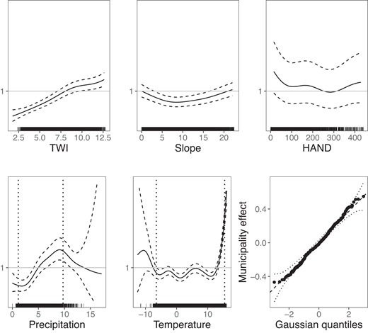
Multiplicative response effects of topographical (first row) and climatological (second row) covariates on water damage risk under the quarterly negative binomial model indicated by the mean effect (solid line) with a 95% confidence band (dashed lines), all on a joint y-axis scale. In-sample covariate values are indicated by black tick marks along the x-axes. For temperature and precipitation, dotted vertical lines show the 1st and 99th percentile, cf. Section 4.3. Bottom right: QQ-plot of the municipality random effect.
During model selection, we also investigated various subsets of property attributes for the building risk component. Of the considered building characteristics, only the variable ‘type of roof’ did not yield predictive power and was removed from the analysis. A basement variable is highly significant, properties with basement exhibiting a substantially higher risk than those without. Moreover, privately inhabited properties such as houses and cabins are at a higher risk of experiencing water damage than industrial or agricultural buildings by approximately an order of magnitude. Finally, the risk contribution from the construction year peaks in the early 1960s. This indicates both that building regulations have improved and that older properties are well capable of withstanding today’s climatic exposure.
4.2 Risk assessment for a stationary climate
As described in Section 3.2, we can decompose our model into several risk factors, corresponding to the groups of covariates. In particular, the model assigns a specific topographical risk and a specific climatological risk to each contract, see equation (2). These factors depend only on the location and not on any contract-specific characteristics. They can therefore be calculated for any location for which topographical/climatological indices are available. Figure 4 shows maps of the corresponding sub-risks, as well as a combined map showing the product for two example areas of km, around the Norwegian cities of Bergen and Tromsø that obtain different risk profiles. The greater Bergen area, famous for heavy rainfall, gets assigned an above-average (that is, ) climatological risk, resulting in an above average combined risk. For Tromsø, the climatological risk and subsequently the combined risk is more varied within the considered region.
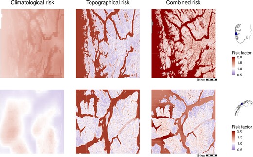
Climatological, topographical, and combined risk factor for the greater Bergen area (top row) and greater Tromsø area (bottom row), see the small maps on the right-hand side for the location of Bergen and Tromsø, respectively. The colourscale is centred at white, corresponding to the average risk, with below-average risk in blue and above-average risk in red.
4.3 Projected risk development due to climate change
We employ 12 regional climate projections under both RCP 4.5 and 8.5 for the two future periods 2031–2060 and 2071–2100 in order to assess risk development due to climate change. It can be observed in Figure 3 that the estimated splines for the climatological variables exhibit implausible behaviour towards the tail of the distribution of the training data. For example, the spline for average daily precipitation decreases starting at 9.5 mm/day. Simultaneously, the uncertainty of the spline increases dramatically, suggesting that this effect likely constitutes an artefact of the statistical model rather than reflecting a causal relationship. This does not have much effect for the risk assessment in the current climate, since only few data points are located within the affected range. In climate projections for future time periods, however, the distribution of the climatological variables is shifted. As a result, the tail estimates of the splines can have much higher impact. To counteract an implausible extrapolation of the model beyond the range of the training data, we regularise the model by freezing the two climatological splines before the 1st percentile and past the 99th percentile of the training data, indicated as vertical dotted lines in Figure 3. This extrapolation issue and associated model assumptions are further discussed in Section 5.
To visualise future projected changes in risk, we consider the ratio of future and present climatological risk factors. Figure 5 shows the 10th, 50th, and 90th percentile of projected risk ratios based on the 12 different climate models. The projections show a significant increase in risk for the west coast up to and including the Lofoten archipelago, as well as for the southeastern part of the country around the capital, Oslo. Towards the end of the century, both RCP scenarios project large areas with increased risk of 25% and higher. Under RCP 8.5, an increase of more than 35% is projected for some areas. None of the considered scenarios project a decrease in risk for any part of the country.
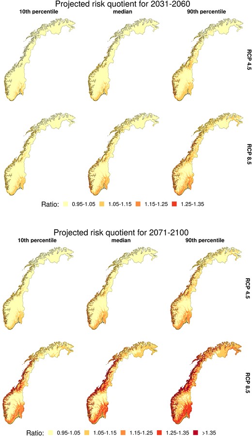
Ratio of projected future climatological risk for 2031–2060 (top) and 2071–2100 (bottom), and historical 1991–2020 climatological risk, see Section 3.2 for a definition. Each column shows pointwise 10th, 50th, and 90th percentiles of the probabilistic projections based on 12 climate models.
The maps shown in Figure 5 are exclusively based on the projected changes in mean quarterly precipitation and surface temperature. Alternatively, we can use our full model to project the change in number of claims per municipality. These projections incorporate topography and building-specific characteristics of the contracts within each municipality and are thus more directly connected to Gjensidige’s portfolio. The resulting projections are shown in Figure 6. These overall ratios are somewhat higher than for the climatological risk in Figure 5, in that a larger overall area has a projected relative change of more than 15% in Figure 6 compared to Figure 5. This effect can partly be explained by the uneven spatial distribution of buildings within the considered municipalities: The majority of Norway’s population lives in coastal areas, where a higher increase of risk is expected according to Figure 5.
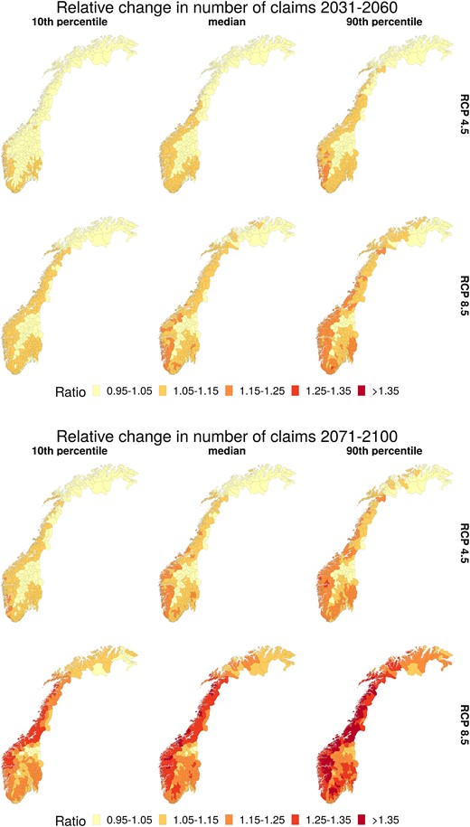
Projected relative change in number of claims for all municipalities in Norway based on climate projections for 2031–2060 (top) and 2071–2100 (bottom) relative to estimates for 2009–2021 based on 1991–2020 climatology. For each future period, the first row is based on climate projections under RCP 4.5 and the second row under RCP 8.5. The columns shows the 10th, 50th, and the 90th percentile (for each municipality) based on 12 climate models.
Figure 7 shows densities of projected relative climatological risk factors across all grid cells covering Norway for the different climate model configurations. The figure shows that these marginal distributions are rather similar between the different climate models for each projection period and RCP scenario. All densities for the future period 2031–2060 as well as densities for 2071–2100 under RCP 4.5 have a mode within the interval , while the projections for 2071–2100 under RCP 8.5 are more diffuse with modes within the interval . Furthermore, the densities are skewed with a heavy upper tail and an increasing skewness for a more pessimistic RCP and/or a time period further in the future.
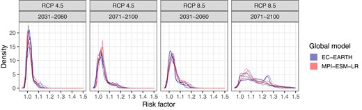
Densities for relative risk factors derived from the climate projections compared to the reference period 1991–2020. Each density represents one climate model configuration (see Table 1), and shows the distribution of projected risk factors across all grid cells covering Norway. The colours of the densities highlight the two different driving GCMs.
We compare our findings to the results of Haug et al. (2011), who modelled the number of claims on the level of municipalities at a daily temporal resolution. That is, they consider a spatially aggregated insurance portfolio and meteorological information at a higher temporal resolution compared to our analysis. This renders use of building-specific covariates impossible, and even if they include hydrological variables like runoff, they do not use topography in their model. Further, Haug et al. (2011) consider a single climate model and are thus only able to capture model uncertainty and not uncertainty due to differences between different climate models. We extend this by considering both uncertainty in model parameters and variability resulting from different climate model configurations (see Table 1). In Figure 8, we show projected future change in the number of claims for three counties considered in Haug et al. (2011).1
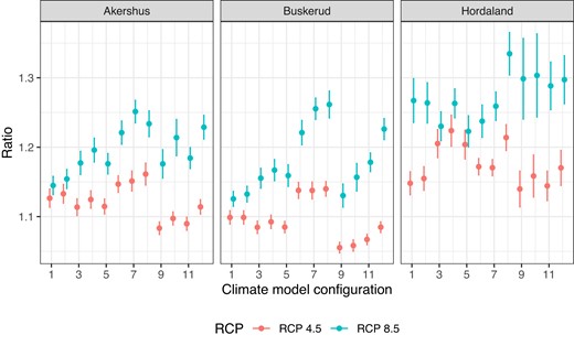
Ratios of change in the number of claims due to climate change under RCP 8.5 and RCP 4.5 for the period 2071–2100 for three counties in Norway. The climate model configuration numbers on the x-axis correspond to the ordering in Table 1. The uncertainty bands are given by twice the standard deviation based on 50 samples from the posterior distribution of the model parameters.
Figure 8 displays the point estimate and approximate 95% confidence intervals for the ratio of expected number of claims in the historical time period compared to 2071–2100. The estimates are based on 50 simulations from a multivariate normal approximation of the posterior distribution of the model parameters. For all counties the variation between the climate model configurations is greater than the variation due to parameter uncertainty, showing that this is an essential part of the overall uncertainty quantification. Our results are not directly comparable to those in Haug et al. (2011) as they use different climate models, emission scenarios, statistical models, and reference period, but some comments are justified. While our projected ratios for Akershus are approximately the same on average as the results reported in Haug et al. (2011), Buskerud, and especially Hordaland, have significantly higher projected ratios in the current setting than previously reported.
5 Discussion
The projection of water damage risk to a future climate involves extrapolating the model in equation (3) beyond the range of the climatological indices for the reference period 1991–2020. As Norwegian climate is expected to get warmer and wetter (Hanssen-Bauer et al., 2009), the extrapolation primarily involves an extrapolation beyond the upper limit of the in-sample values, see Figure 3. The projections presented in Section 4.3 are based on splines truncated at the 1st and 99th percentile of the in-sample distribution of covariate values. In order to assess the effect of this modelling choice, we have also formed water damage risk projections using a linear model for the climatological covariate effect applied with or without truncation, as well as models that only use a precipitation index rather than both precipitation and temperature indices. A model comparison is shown in Figure 9. Figure 9 shows that the modelling choice presented in Section 4.3 is the least conservative of the considered options. In particular, we see that the projected increase in water damage risk is, to a large extent, driven by the inclusion of a temperature index. However, a comparison of the predictive performance of these models in the current climate through a cross-validation study as presented in Section 4.1 shows that the non-linear splines with both temperature- and precipitation-based indices significantly outperforms the other modelling options (results not shown).
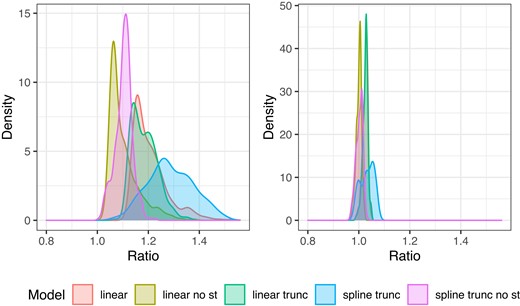
Left: Densities of 90th percentile of relative change in number of claims due to climate change under RCP 8.5 for the period 2071–2100 across all gridpoints in Norway. Right: Densities of 10th percentile of relative change in number of claims due to climate change under RCP 4.5 for the period 2031–2060 across all gridpoints in Norway. Each colour represents projections from different regression models: spline represents the model described in Section 3, linear means that the effect of precipitation and surface temperature is linear on log scale, trunc means precipitation and surface temperature is truncated at the 1st and 99th percentile of the training data, and no st means that surface temperature is excluded from the model.
In Figure 3, we see a steep increase in the spline for high temperatures. Physically, there is no immediate explanation why high temperatures should generate more claims. Thus, these temperatures most likely act as a proxy for some other phenomenon expressed in the data. One hypothesis would be that high surface temperatures are associated with more frequent cloud bursts typically seen during the warm season and in particular on hot days (local, convective precipitation). In urban areas, such events are known to bring potential risk of vast water damage due to a high proportion of non-porous surfaces, often in combination with limited capacity of the sewer system. Claims generated from such conditions will possibly ascribe high values of the temperature variable as the key source for their occurrence. Rural areas also experience hot days with cloud bursts, on average to the same extent as urban areas. Buildings in rural areas are less vulnerable to these events and, for these areas, we would expect the spline to have less of a steep increase for high temperatures. However, as the majority of the buildings in the insurance portfolio are situated in urban areas, the model estimates are formed primarily from the pattern of urban claims.
In a study of water damages in Switzerland, Bernet et al. (2019) show that critical thresholds for precipitation events vary substantially across complex terrain. The models presented in Section 3 assume that a certain level of quarterly precipitation and temperature has the same effect on damage risk everywhere in Norway, cf. Figure 3. Similar to Switzerland, there are substantial country-wide differences in climate. In particular, the amount and type of precipitation observed along the west coast is quite different from that observed, e.g. in the Oslo region on the east side (Hanssen-Bauer et al., 2009). To account for this, building traditions and wastewater collection systems vary across the country. We thus investigated models with spatially varying effects of precipitation and temperature. However, we found that this added model complexity yields poorer predictive performance which we believe to be due to overfitting. The climatic variability (and its impact on building and infrastructure traditions) is one of several effects that are implicitly accounted for by the county and municipality effects. Infrastructure adaptation to local climate might also partially explain why the response effect of precipitation is not monotonically increasing, cf. Figure 3. It should be noted that future projections for risk are made conditional on the current infrastructure in each municipality or county.
The majority of studies that model the effect of weather on insurance risk consider spatially aggregated claims data, see introduction for references. We take a different approach, modelling each property and location separately, but aggregating weather variables over longer time spans. This has the major advantage that it allows to incorporate building-specific covariates, such as whether the property has a basement or not. Moreover, a spatially disaggregated model is required to include the effect of local topography, since variables such as slope vary rapidly in space and quickly lose accuracy when they are spatially averaged. Our analysis shows that including both topographic and building-specific covariates substantially improves the predictive skill of the model. Moreover, risk models applied by insurance companies generally include building-specific information. This makes it challenging in practice to include information from spatially aggregated models into operational risk models.
On the other hand, using temporally aggregated weather data comes with the disadvantage that the model cannot learn from clusters of claims that are associated with heavy rainfall events. However, the aggregation of weather data in time is appropriate for predicting changes in risk due to climate change. Climate models generally aim to project changes in the distribution of weather rather than to provide accurate predictions of daily future weather. We did explore models putting more emphasis on aggregate measures of weather extremes rather than average weather variables (results not shown). For example, we fitted models considering the 95th and 99th percentile of local rainfall. Such models generally did not perform better than models based on average precipitation. The likely reason is that such indices are generally strongly correlated with average precipitation (in our data correlations were typically around ).
During our research, we also experimented with models that neither aggregate in space nor time, i.e. targeting the binary response whether a claim happened for a specific property on a given day. While such models are in principle feasible for the data sets considered here, they are much more computationally costly. Moreover, the resulting models tended to be sensitive to outliers in the weather. This resulted in occasionally unreasonably high probabilities for a claim of 90% or higher for single properties at days with extreme precipitation, in particular when future climate projections were considered.
6 Conclusions
This paper proposes a nationwide model for risk of rainfall-induced water damage in Norway. The model incorporates local topographical and climatological information as well as contract-specific property data. The overall risk assessment can be decomposed into several factors which, in particular, allows for the derivation of topographical and climatological risk maps covering the entire country. Climate projections yield projections for changes in water damage risk in future decades due to climate change. Based on a multi-model ensemble of regional climate projections, we project a spatially varying increase in risk of as much as 25% for large areas towards the end of this century.
Insurance companies’ risk models materialise in tariffs that price the individual customer and the individual object. Historical damages and losses—including those caused by pluvial flooding—form the basis for the tariffs, and trends together with knowledge of future changes make the tariffs predictive. The results of this study improve the pricing quality in multiple ways. Gjensidige will gain knowledge about future developments in the overall level of losses, the geographical loss distribution related to present and future climate and the risk level of individual buildings due to their location in the terrain. These are aspects that expand and challenge current risk assessment practice in the insurance sector. The model provides not only precise risk information for Gjensidige’s existing customers but also any potential new object—built or planned—in Gjensidige’s future portfolio. All of this is crucial information for pricing according to risk at both portfolio and customer level.
Risk associated with climate and climate change plays a special role compared to other risks due to global efforts for climate change adaptation and mitigation. The risk models that have been developed here provide Gjensidige with a basis for redistribution of premiums at building level (topography) and future redistribution and adaptation at geographical level. More importantly, the new knowledge can be utilised to reduce risk for both municipalities and individual customers, supporting and furthering a sustainable business strategy. Municipalities can gain valuable insights regarding investment priorities such as upgrades of sewerage networks or planning of new residential or commercial areas. Gjensidige will also seek to use the results to develop preventive measures that customers can implement themselves.
After an earlier trial period, Norwegian insurance companies will from 2022 provide claims data related to weather and climate to the Norwegian authorities. The purpose of this programme is for the municipalities to get an overview of areas with high-risk exposure so that measures can be taken where they are expected to have the greatest effect. The results of the current study provide valuable knowledge regarding expected future changes in this context. Models of the type presented here can help ensure that measures are prioritised to provide the greatest possible societal benefit, both by preventing economic and social costs and because every damage entails a CO cost. The most effective climate change adaptation and mitigation strategy for an insurance company is to prevent damage occurrence.
Acknowledgments
We thank Andreas Lura for extracting the insurance data, Magne Aldrin for helpful discussions and Annabelle Redelmeier for help with the manuscript. Moreover, we would like to thank the associate editor and an anonymous reviewer for their suggestions which helped to improve the content of the paper.
Data availability
Our analysis utilizes four different datasets, the details of which can be found in Section 2. The insurance data is not publicly available due to its confidential nature. The topography data is generated from a freely accessible Digital Elevation Model, generated by the Norwegian Mapping Authorities (Kartverket), and is available at https://hoydedata.no. The meteorological data (seNorge version 2018), produced by the Norwegian Meteorological Service, is available at https://thredds.met.no/thredds/catalog/senorge/seNorge_2018/. Finally, the regional climate projections we use are provided by the EURO-CORDEX initiative and freely available. For information on how to access this data, please visit https://cordex.org/.
References
Footnotes
Haug et al. (2011) compare Akershus, Buskerud, and Hordaland, counties that no longer exist due to a restructuring of counties in 2020. For comparison, we derive predictions for these old counties by averaging predictions for all properties lying within the old county borders.
Author notes
*Read before The Royal Statistical Society at the first meeting on ‘Statistical aspects of climate change' held at the Society’s 2022 annual conference in Aberdeen on Wednesday, 14 September 2022, the President, Professor Sylvia Richardson, in the Chair.
