


Abstract
Customer churn is one of the most important concerns for large companies. Currently, massive data are often encountered in customer churn analysis, which bring new challenges for model computation. To cope with these concerns, sub-sampling methods are often used to accomplish data analysis tasks of large scale. To cover more informative samples in one sampling round, classic sub-sampling methods need to compute sampling probabilities for all data points. However, this method creates a huge computational burden for data sets of large scale and therefore, is not applicable in practice. In this study, we propose a sequential one-step (SOS) estimation method based on repeated sub-sampling data sets. In the SOS method, data points need to be sampled only with probabilities, and the sampling step is conducted repeatedly. In each sampling step, a new estimate is computed via one-step updating based on the newly sampled data points. This leads to a sequence of estimates, of which the final SOS estimate is their average. We theoretically show that both the bias and the standard error of the SOS estimator can decrease with increasing sub-sampling sizes or sub-sampling times. The finite sample SOS performances are assessed through simulations. Finally, we apply this SOS method to analyse a real large-scale customer churn data set in a securities company. The results show that the SOS method has good interpretability and prediction power in this real application.
1 INTRODUCTION
Customer churn is one of the most important concerns for large companies (Ascarza et al., 2018; Kayaalp, 2017). With increasingly fierce competition, it is important for companies to retain existing customers and prevent potential customer churn. Customer churn often refers to a situation in which customers no longer buy or use a company's products or services. For each customer, to churn or not to churn is a typical binary indicator. Therefore, customer churn prediction is often considered as a classification task, and several classifier models have been applied to address this issue (Ahmad et al., 2019). Among the previous models, logistic regression is widely used owing to its good interpretability (Ahn et al., 2019; Maldonado et al., 2021). Therefore, in this work, we employ logistic regression models to handle the task of customer churn analysis.
With the arrival of the ‘Big Data’ era, massive data are often encountered in customer churn analysis. For example, the real data analysed in this work comprise 12 million transaction records from 230,000 customers, which take up 300 GB in total. Such large amounts of data present great challenges for customer churn analysis. The first concern is memory constraint. The data can be too large to be stored in a computer's memory, and hence, have to remain stored on a hard drive. The second challenge is computational cost. For massive data, even a simple analysis (e.g., mean calculation) can take a long time. These challenges create large barriers for customer churn analysis with massive data.
To cope with these challenges, modern statistical analysis for massive data is developing fast. Basically, there are two streams of approaches for massive data. The first stream considers storing data in a distributed system and then applying the ‘divide-and-conquer’ strategy to accomplish data analysis tasks of huge scales. See McDonald et al. (2009), Lee et al. (2017), Battey et al. (2018), Jordan et al. (2019), Zhu et al. (2021), Wang et al. (2021), and the references therein. Another stream uses sub-sampling techniques that conduct calculations on sub-samples drawn from the whole data set to reduce both memory cost and computational cost. Important works include, but are not limited to, Dhillon et al. (2013), Ma et al. (2015), Wang et al. (2018), Quiroz et al. (2019), Ma et al. (2020), and Yu et al. (2020).
It is remarkable that there are big differences in the two streams of approaches. The distributed methods usually require typical equipment support. For example, a distributed system is often required, which consists of one central computer served as Master and all other computers served as Workers. Then, the goal of distributed methods is to obtain an estimator based on the whole sample. However, the sub-sampling methods can be conducted using one single computer. They focus on the approximation of the whole sample estimator based on sub-samples with limited resources. In this customer churn application, we do not have equipment support for distributed analysis. Therefore, in this work, we focus on sub-sampling methods to handle the customer churn analysis with massive data.
Classic sub-sampling methods require only one round of data sampling. To cover more informative samples in the single sampling round, non-uniform sampling probabilities are often specified for each data point, so that more informative data points can be sampled with higher probabilities. Typical approaches include leverage score-based sub-sampling (Drineas et al., 2011; Ma et al., 2015; Ma & Sun, 2015), information-based optimal sub-data selection (Wang et al., 2019), the optimal Poisson sampling method, and its distributed implementation (Wang et al., 2021), among others. These sub-sampling estimators have been proved to be consistent and asymptotically normal under appropriate regularity conditions; see Ma et al. (2020) for an important example. However, for these non-uniform sub-sampling methods, the step of evaluating non-uniform sampling probabilities for the whole data set would create a huge computational burden. For example, Wang et al. (2018) proposed optimal sub-sampling methods motivated by the A-optimality criterion (OSMAC) for large sample logistic regression. To find the optimal sub-sampling probabilities in the OSMAC method, the computational complexity is for a data set with observations and -dimensional covariates. Consequently, this optimal sub-sampling algorithm could be computationally very expensive when is very large. In the customer churn application, the whole data size is about 12 million. It would not be computationally feasible for the previous sub-sampling methods to handle this task.
An obvious way to address this problem would be to sample sub-data with uniform probabilities while operating the sub-sampling step repeatedly. By sampling with uniform probabilities, we are free from computing probabilities for the whole data set in advance, which can largely alleviate the computational burden. By sampling repeatedly, the sampled data would be close to the whole data set. In an ideal situation, if we were to conduct sub-sampling without replacement, then sampling times would cover the whole data set, where and are the sizes of the whole data and sub-data, respectively. It is as if the whole data were stored in a distributed system.
The sub-sampling cost cannot be negligible, especially for repeated sub-sampling methods. It is remarkable that the time needed to sample one data point from the hard drive mainly consists of two parts. The first is the addressing cost, which is the time taken to identify the target data point on the hard drive. The second is the I/O cost, which is the time needed to read the target data point into the computer memory. Both are hard drive sampling costs, which cannot be ignored when we apply sub-sampling methods to massive data sets. Therefore, inspired by Pan et al. (2020), we adopt the sequential addressing sampling method to reduce the hard drive sampling cost. When data are randomly distributed on a hard drive, for each sub-data, only one starting point is selected and the other data points can be obtained sequentially from the starting point. In this way, the addressing cost can be reduced substantially for sub-sampling methods.
Based on the repeated sub-sampling data sets from the whole customer churn data, it is worthwhile to consider how to obtain an efficient customer churn estimation for both statistical property and computational cost. To this end, we propose a sequential one-step (SOS) method, whose estimation bias and variance can both be reduced by increasing the total sub-sampling times . Specifically, in the first sub-sampling step, we can obtain an estimate based on the first sub-data using, for example, the traditional Newton–Raphson algorithm. Then, in the second sub-sampling step, we regard as the initial value, and conduct only one-step updating based on the second sub-data. This leads to . In the next step, the average of the first two estimates, that is, , is regarded as the initial value, and one-step updating based on the third sub-data is conducted again to obtain . In summary, in the (k+1)th step, the average of all previous estimates (i.e., ) serves as the initial value, and one-step updating based on the newly sampled sub-data is conducted to obtain the estimate . The final estimate of sub-sampling steps is the average of all estimates, that is, .
It is noteworthy that, except for the first sub-sampling step, SOS requires only one round of updating in the subsequent sub-sampling steps. Therefore, it is computationally efficient. We also establish theoretical properties of the SOS estimator. We prove that both the bias and variance of the SOS estimator can be reduced as the sampling times increase. We conduct extensive numerical studies based on simulated data sets to verify our theoretical findings. Finally, the SOS method is applied to the customer churn data set in a securities company to demonstrate its application.
The rest of this article is organised as follows. Section 2 introduces the SOS method. Section 3 presents simulation analysis to demonstrate the finite sample performance of the SOS estimators. Section 4 presents a real application for customer churn analysis using the SOS method. Section 5 concludes with a brief discussion.
2 SOS ESTIMATOR BY SUB-SAMPLING
2.1 Basic notations
Assume we have all the sample observations, , where is defined as the whole sample size. Define to be the observation collected from the ith observation, where is the response and is the associated predictor. Conditional on , assume that is independently and identically distributed with density function , where , is the unknown parameter, and is an open subset in . We assume for convenience. To estimate the unknown parameter , the log-likelihood function can be spelled out as
where is the log-likelihood function. For convenience, we use to denote hereafter.
Note that when is quite large, the whole data set is often kept on a hard drive, and cannot be read into the memory as a whole. Then it would be time consuming to select a sample randomly from the hard drive into the computer memory. To save time, we apply the sequential addressing sub-sampling (SAS) method (Pan et al., 2020) to conduct the sub-sampling directly on hard drive, not memory. To apply the SAS method, the whole data should be randomly distributed on the hard drive. Otherwise, a shuffle operator would be needed to make data randomly distributed. The detailed implementation process of conducting shuffle operation can be found in Appendix A in Data S1. Then, the sub-sampling steps can be performed iteratively based on the randomly distributed data to obtain sub-samples. Next, we describe the SAS method in detail.
First, one data point should be randomly selected on the hard drive as a starting point, that is, , where is the desired sub-data size. This yields marginal addressing cost, as only one data point is chosen. Second, with a fixed starting point, the sub-sample with size is selected sequentially with index . These selected sub-samples are collected as . Except for the first starting point indexed by , the remaining data points are sampled sequentially. Therefore, no additional addressing cost is required, and the total sampling cost can be reduced substantially.
It is notable that, although the SAS method serves as a preparing step for the SOS method, there are fundamental differences between SAS and SOS. The SAS method is actually a sub-sampling technique, which can sample data directly from the hard drive and save much addressing cost. Based on the SAS sub-samples, Pan et al. (2020) also study the theoretical properties of some basic statistics estimators (e.g., sample mean). However in SOS, we focus on the estimation problem of logistic regression and discuss updating strategy to exploit the sub-samples obtained by SAS. It is remarkable that, the SAS method only serves as a tool for fast sampling, and the theoretical properties of the SOS estimator could still be guaranteed without this sampling step.
2.2 SOS estimator
Assume the whole data set is randomly distributed on the hard drive. Then, the SAS method can be applied for fast sub-sampling. Recall that the sub-sample size is . By the SAS method, a total of different sequential sub-samples can be generated. Assuming that the sub-sampling is repeated times, in the kth sub-sampling, the sub-sample can be selected with replacement. We further denote as the indexes of data points in . Based on with , we propose the SOS method for efficient estimation of .
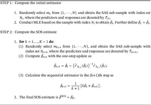
To obtain the SOS estimator, an initial estimator is first calculated based on one of the SAS sub-samples with the index set denoted as . For example, it may be a maximum likelihood estimator (MLE). Then, in the (k+1)th sub-sampling step with , a new SAS sub-sample can be obtained as . Based on the (k+1)th sub-sample, we conduct the following two steps iteratively to obtain the SOS estimator. The details of the SOS method are shown in Algorithm 1. Recall we have assumed that, the whole data are already shuffled or randomly distributed before we begin the SOS procedure. Step 1: One-step update. Assume that the initial estimator in this step is . Then, we conduct one-step updating based on to obtain the one-step updated estimator in this step, that is,
where and are the first- and second-order derivatives of the likelihood function based on the kth sub-sample, respectively. Step 2: Average. The SOS sub-sampling estimator for the (k+1)th step can be calculated as
Conduct Steps 1 and 2 iteratively. The estimator obtained in the Kth step is the final SOS estimator, that is, . See Figure 1 for an illustration of calculating the SOS estimator based on the SAS sub-sampling method.
Algorithm 1. SOS estimation algorithm
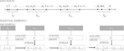
Illustration of the sequential one-step estimator based on random addressing sub-sampling
Remark: We offer two remarks here about the SOS estimator. First, for each sub-sample, only the one-step update is conducted by (1). This may yield marginal computational cost because (1) the sample size is relatively small; and (2) no Newton–Raphson-type iterations are involved. It is notable that, there is no need to achieve fully Newton–Raphson convergence for each sub-sample. This is because the Newton–Raphson algorithm is not affected by the initial value when it goes to convergence. Therefore, if the sub-sample estimator is not one-step updating, but obtained with fully Newton–Raphson convergence, then the initial value would not affect the resulting estimator in the (k+1)th sub-sample. Consequently, the SOS estimator degenerates to the one-shot (OS) estimator, which we theoretically compare in the next sub-section. Second, each can be viewed as the average of the one-step estimator in form (1) for the first steps. This leads to some nice properties: (1) a total of sub-samples are used in the estimation; and (2) the standard error of the final estimator can be reduced by averaging. More weighting schemes could be considered in the SOS updating strategy; see the weighting scheme in the aggregated estimating equation (AEE) method (Lin & Xi, 2011) for an example.
It is also notable that, our proposed SOS method is an extension of the classical one-step estimator (Shao, 2003; Zou & Li, 2008) in the field of sub-sampling. For example, Zhu et al. (2021) has developed a distributed least squares approximation (DLSA) method to solve regression problems on distributed systems. In the DLSA method, once the weighted least squares estimator (WLSE) is obtained by the Master, it would be broadcast to all Workers. Then each Worker would perform a one-step iteration using the WLSE as the initial value to obtain a new estimator. Another work is Wang et al. (2021), who propose a one-step upgraded pilot method for non-uniformly and non-randomly distributed data. However, both the two methods are divide-and-conquer (DC) type methods, which are quite different from the sub-sampling methods. For example, one typical difference is that, in DC methods, the estimators from different Workers can be regarded as independent. However, in our SOS method, the estimators to are sequentially obtained, which makes them dependent with each other. This leads to challenges in investigation of the asymptotic theory for the SOS estimator. More differences between the divide-and-conquer type methods and sub-sampling methods can be found in the Appendix B in Data S1.
2.3 Theoretical properties of the SOS estimator
We further investigate the properties of the SOS estimator in this subsection. To establish the theoretical properties of the SOS estimator, assume that is an open subset in the Euclidean space, and we have the following conditions.
- (C1)
The sub-sample size , the whole sample size , and the sub-sampling steps satisfy that as , , and .
- (C2)
Assume that the first- and second-order derivatives of log-likelihood satisfy equations , and , for .
- (C3)
Assume that is finite and positive definite at , where is the true parameter.
- (C4)
There is an open subset of that contains the true parameter , such that for all s, exists for all , and . Moreover, assume function exists, such that for any , we have , where is a constant. For and , we have
- (C5)
Assume the covariates s independently follow Gaussian distributions.
Condition (C1) restricts the relationships of and . By the condition, we know that the sub-sampling times should not grow too fast in the sense that , and the sub-sampling size should not increase too fast in the sense that Conditions (C2)–(C4) are standard regularity conditions. They are commonly adopted to guarantee asymptotic normality of the ordinary maximum likelihood estimates; see, for example, Lehmann and Casella (1998) and Fan and Li (2001). Condition (C5) is a classical assumption on covariates (Wang, 2009).
With the conditions satisfied, we can establish the properties of , which equals . Define , and . Then, the following theorem holds.
Theorem 1Assume conditions (C1)–(C5) hold. Then, we have (1)with, and. (2)
The proof of Theorem 1 is in Appendix B.1. As shown in Theorem 1, we separate the difference between the SOS estimator and the true parameter into two parts, the bias term and variance term. One could note that the bias term and variance term are both determined by two main parts. The first part is related to the whole sample size . This part cannot disappear by using the SOS procedure. The second term is , which is affected by the SOS procedure and can decrease with larger or . In addition, the SOS estimator satisfies asymptotic normality with asymptotic variance . In particular, when is much larger than , it could achieve the same statistical efficiency as the global estimator. Note that the practical demand for estimation precision is usually limited. On the contrary, the budget for sampling cost is very valuable. Then, it may be more appealing to sacrifice the statistical efficiency to some extent for lower sampling cost. Therefore, in practice, we often expect the SOS method to be implemented with reasonably large and (i.e., ) as long as the desired statistical precision is achieved.
For theoretical comparison, we introduce a simple alternative method. For each sub-sample , we separately compute the MLE . Then, all sub-sample estimators are simply averaged to obtain the OS estimator. Let denote the OS estimator. We obtain the following conclusion.
Proposition 1For the OS estimator, under the same conditions in Theorem 1, we have, where. Further assumethen, we have
The proof of Proposition 1 is in Appendix B.2. Comparing Theorem 1 and Proposition 1, we find that the leading terms for the variance of both the SOS and the OS estimators are identical. However, the bias term of the OS estimator is of order , which cannot be improved as increases. By contrast, the bias of the SOS estimator is , which can be significantly reduced as increases. Therefore, compared with the SOS estimator , requires a more stringent condition , such that it could achieve the same asymptotic normality as the global estimator (Huang & Huo, 2019; Jordan et al., 2019). However, this condition is not necessary for the SOS estimator.
Next, to make an automatic inference, we discuss the estimation of the standard error of the SOS estimator. Specifically, based on the SOS procedure, we construct the following statistic as
The properties of are presented in the following theorem.
Theorem 2Under the same conditions in Theorem1, we have
The proof of Theorem 2 is in Appendix B.3. We conclude that the leading orders of and are the same. However, as an estimator of , is biassed, but the order of the bias is , which decreases as increases or decreases. Practically, the unknown parameter in can be replaced by to obtain and . Then, can be calculated based on and in the form of (2). Note that by Theorem 1, the leading term for the variance of is . Such term can be consistently estimated by the proposed SE estimator . Its asymptotic property is presented in the following theorem.
Theorem 3Under the same conditions in Theorem 1, we have
(3)
The proof of Theorem 3 is in Appendix B.4. Combining the results of Theorems 1 and 3, we immediately obtain that As a result, both the estimator and statistical inference could be easily and efficiently derived by our SOS procedure. We illustrate the performance of the SOS estimator and in the next section.
3 SIMULATION STUDIES
3.1 Simulation design
To demonstrate the finite sample performance of the SOS estimator, we present a variety of simulation studies. Assume that the whole data set contains observations. For , we generate each observation under the logistic regression model. We choose the logistic regression model because it is a specific model used for customer churn analysis. Given that the SOS method can be extended easily to other generalised regression models, we also choose the Poisson regression model as an example to test the effectiveness of the SOS method. The specific settings for the two model examples are as follows.
Example 1(Logistic regression
Logistic regression is used to model binary responses. In this example, we consider exogenous covariates , where each covariate is generated from a standard normal distribution . We set the coefficients for as . Then, the response is generated from a Bernoulli distribution with the probability given as
Example 2(Poisson regression)
Poisson regression is used to deal with count responses. We also consider exogenous covariates, which are all generated from standard normal distribution. The corresponding coefficients are set as . Then, the response is generated from a Poisson distribution given as
After obtaining observations, we consider combinations of different sub-sampling size and different sub-sampling times. In both logistic and Poisson regression examples, we set . Then in the logistic regression example, we consider cases of small , and set . In the Poisson regression example, we consider cases of big , and set . In each combination of and , we repeat the experiment times.
3.2 Comparison with repeated sub-sampling methods
In this sub-section, we compare the proposed SOS estimator with the OS estimator, which is representative of the repeated sub-sampling methods. Specifically, in each simulated data set, we obtain the SOS estimator using Algorithm 1. For the OS estimator, we first randomly obtain sub-data, and then independently apply the Newton–Raphson method to each sub-data. Specifically, in the kth sub-data, we set the initial value as , and then fully conduct the Newton–Raphson method to obtain estimate . The final OS estimator is calculated as . For one particular method (i.e., SOS and OS), we define as the estimator in the bth () replication. Then, to evaluate the estimation efficiency of each estimator, we calculate the bias as , where . The standard error () can be estimated based on Theorem 2 for the SOS method. We report the average . Then, we compare with the Monte Carlo SD of , which is calculated by . Next, we construct a 95% confidence interval for as , where is the lower quantile of a standard normal distribution. Then, the coverage probability is computed as , where is the indicator function. Last, we compare the computational efficiency of the two methods. It is notable that, for a fixed sample size , the computational time consumed by each Newton–Raphson iteration is the same for the SOS and OS methods. Therefore, we use the average round of Newton–Raphson iterations to compare the computational efficiency of the SOS and OS methods.
Tables 1 and 2 present the simulation results for estimation performance under the logistic regression and Poisson regression, respectively. In general, the simulation results under the two examples are similar. We draw the following conclusions. First, as the sub-sampling times increases, the bias of the SOS estimator becomes much smaller than that of the OS estimator. This is because the bias of the SOS estimator decreases with increasing , while the bias of the OS estimator is always . Second, the and of both estimators decrease with increasing or , implying that the two estimators are consistent. Third, as the bias and of the SOS estimator can decrease with and , the bias always behaves negligibly compared with . However, the bias of the OS estimator is comparable to or even larger than its ; see in Table 2 for an example. Next, the empirical coverage probabilities of the SOS estimator are all around the nominal level of 95%, which suggests that the true SE can be well approximated by its estimators derived in Theorem 2. However, the empirical coverage probabilities of the OS estimator show a deceasing trend when enlarging . This is because the bias of the OS estimator cannot be negligible when is large. Last, regarding the computational time, we compare the average rounds of Newton–Raphson iterations consumed by the two methods. Except for the initial sub-sample estimator, the SOS method uses only one Newton–Raphson update for each subsequent sub-sample. However, on average, the OS estimator requires seven or eight rounds of Newton–Raphson updates to obtain convergence. Therefore, the SOS estimator is computationally more efficient than the OS estimator.
Simulation results for estimation performance under logistic regression
| Bias × | SE × | ECP | ROUND | |||||||
|---|---|---|---|---|---|---|---|---|---|---|
| SOS | OS | SOS | OS | SOS | OS | SOS | OS | SOS | OS | |
| 10 | 0.532 | 0.903 | 6.598 | 7.237 | 6.545 | 6.596 | 0.952 | 0.912 | 1.875 | 7.145 |
| 20 | 0.336 | 0.963 | 4.694 | 5.109 | 4.687 | 4.717 | 0.947 | 0.879 | 1.923 | 7.492 |
| 30 | 0.204 | 0.943 | 3.815 | 4.142 | 3.857 | 3.88 | 0.950 | 0.858 | 1.884 | 7.146 |
| 40 | 0.170 | 0.976 | 3.278 | 3.559 | 3.359 | 3.379 | 0.950 | 0.858 | 1.821 | 7.240 |
| 50 | 0.150 | 0.915 | 2.997 | 3.247 | 3.015 | 3.032 | 0.954 | 0.823 | 2.122 | 7.654 |
| 100 | 0.058 | 0.921 | 2.124 | 2.293 | 2.162 | 2.173 | 0.955 | 0.755 | 1.942 | 7.149 |
| 10 | 0.291 | 0.545 | 4.709 | 4.923 | 4.539 | 4.554 | 0.946 | 0.927 | 1.873 | 7.364 |
| 20 | 0.160 | 0.479 | 3.233 | 3.374 | 3.283 | 3.293 | 0.952 | 0.919 | 1.917 | 7.381 |
| 30 | 0.098 | 0.420 | 2.682 | 2.793 | 2.707 | 2.714 | 0.950 | 0.912 | 1.921 | 7.399 |
| 40 | 0.065 | 0.453 | 2.328 | 2.422 | 2.363 | 2.370 | 0.954 | 0.906 | 1.893 | 7.416 |
| 50 | 0.043 | 0.438 | 2.080 | 2.161 | 2.125 | 2.130 | 0.951 | 0.904 | 1.834 | 7.433 |
| 100 | 0.041 | 0.448 | 1.550 | 1.609 | 1.553 | 1.556 | 0.948 | 0.882 | 1.985 | 7.450 |
| 10 | 0.119 | 0.245 | 3.198 | 3.269 | 3.200 | 3.205 | 0.950 | 0.938 | 1.881 | 7.467 |
| 20 | 0.055 | 0.239 | 2.285 | 2.331 | 2.322 | 2.325 | 0.952 | 0.938 | 1.954 | 7.484 |
| 30 | 0.046 | 0.224 | 1.891 | 1.926 | 1.926 | 1.928 | 0.951 | 0.936 | 2.016 | 7.501 |
| 40 | 0.035 | 0.218 | 1.681 | 1.714 | 1.689 | 1.692 | 0.949 | 0.934 | 1.982 | 7.519 |
| 50 | 0.031 | 0.226 | 1.529 | 1.558 | 1.532 | 1.534 | 0.947 | 0.929 | 2.104 | 7.536 |
| 100 | 0.020 | 0.237 | 1.148 | 1.170 | 1.150 | 1.151 | 0.947 | 0.912 | 2.163 | 7.553 |
Notes: The bias, SE, , and ECP are reported for the sequential one-step (SOS) and one-shot (OS) estimators, respectively. The average Newton–Raphson rounds (representing the computational time) of the two estimators are also reported.
Simulation results for estimation performance under Poisson regression
| Bias | SE | ECP | ROUND | |||||||
|---|---|---|---|---|---|---|---|---|---|---|
| SOS | OS | SOS | OS | SOS | OS | SOS | OS | SOS | OS | |
| 100 | 0.063 | 3.656 | 3.237 | 3.437 | 3.237 | 3.505 | 0.951 | 0.820 | 1.892 | 8.669 |
| 200 | 0.042 | 3.649 | 2.329 | 2.478 | 2.365 | 2.555 | 0.951 | 0.711 | 1.934 | 8.673 |
| 300 | 0.035 | 3.594 | 1.947 | 2.085 | 1.989 | 2.148 | 0.955 | 0.634 | 1.910 | 8.671 |
| 400 | 0.033 | 3.599 | 1.720 | 1.839 | 1.770 | 1.910 | 0.959 | 0.571 | 1.907 | 8.671 |
| 500 | 0.031 | 3.597 | 1.564 | 1.667 | 1.625 | 1.754 | 0.959 | 0.524 | 1.907 | 8.671 |
| 1000 | 0.033 | 3.593 | 1.222 | 1.294 | 1.286 | 1.387 | 0.960 | 0.426 | 1.893 | 8.670 |
| 100 | 0.039 | 1.275 | 2.096 | 2.138 | 2.103 | 2.167 | 0.950 | 0.912 | 1.884 | 8.326 |
| 200 | 0.034 | 1.241 | 1.555 | 1.584 | 1.575 | 1.622 | 0.957 | 0.879 | 1.892 | 8.323 |
| 300 | 0.030 | 1.234 | 1.315 | 1.337 | 1.353 | 1.393 | 0.958 | 0.856 | 1.927 | 8.322 |
| 400 | 0.026 | 1.241 | 1.194 | 1.214 | 1.226 | 1.262 | 0.961 | 0.834 | 1.962 | 8.323 |
| 500 | 0.026 | 1.241 | 1.115 | 1.135 | 1.143 | 1.176 | 0.960 | 0.816 | 2.043 | 8.322 |
| 1000 | 0.023 | 1.239 | 0.923 | 0.936 | 0.956 | 0.984 | 0.958 | 0.765 | 1.895 | 8.321 |
| 100 | 0.038 | 0.485 | 1.466 | 1.476 | 1.470 | 1.489 | 0.947 | 0.932 | 1.884 | 8.153 |
| 200 | 0.035 | 0.485 | 1.131 | 1.137 | 1.145 | 1.160 | 0.956 | 0.932 | 1.892 | 8.153 |
| 300 | 0.032 | 0.498 | 1.006 | 1.012 | 1.013 | 1.026 | 0.953 | 0.920 | 1.903 | 8.153 |
| 400 | 0.034 | 0.485 | 0.935 | 0.939 | 0.940 | 0.952 | 0.951 | 0.915 | 1.906 | 8.153 |
| 500 | 0.032 | 0.488 | 0.882 | 0.886 | 0.894 | 0.905 | 0.953 | 0.917 | 1.891 | 8.152 |
| 1000 | 0.026 | 0.486 | 0.769 | 0.772 | 0.792 | 0.802 | 0.954 | 0.910 | 1.902 | 8.152 |
Notes: The bias, SE, , and ECP are reported for the sequential one-step (SOS) and one-shot (OS) estimators, respectively. The average Newton–Raphson rounds (representing the computational time) of the two estimators are also reported.
3.3 Comparison with non-uniform sub-sampling methods
In this sub-section, we compare the proposed SOS method with the non-uniform sub-sampling methods. To this end, we choose the OSMAC method (Wang et al., 2018) for the comparison, which is particularly designed for large sample logistic regression. The OSMAC method applies a two-step algorithm for the model estimation. In the first step, a pilot sample of size is randomly chosen to obtain a pilot estimate. Then, the pilot estimate is used to compute the optimal sub-sampling probabilities for the whole data. In the second step, a new sub-sample of size is chosen based on the optimal sub-sampling probabilities. Then, the final OSMAC estimate is obtained using the total samples. We compare the two methods under the logistic regression example. To mimic a large data set, we consider the whole sample size . For fixed , the whole data set is generated under the logistic regression model following the procedures in Section 3.1.
Below, we compare the SOS method and OSMAC method under one specific situation. That is, the compute memory is limited, which could only support building a logistic regression model for a sample with size . In this situation, the sub-sample size used in SOS is fixed as , and we vary the sub-sampling times as . As for the OSMAC method, we set and . The OSMAC method is implemented using the corresponding R package provided by Wang et al. (2018).
For a reliable comparison, the experiment is randomly replicated for times for each experimental setup. We use the mean squared error (MSE) to evaluate the statistical efficiencies of the two methods. Specifically, for one particular method (i.e., SOS and OSMAC), we define as the estimator in the bth () replication. Then, the MSE of each estimator is computed as . We also compare the computational time of the two methods. All experiments are conducted on a server with 12 Xeon Gold 6271 CPU and 64 GB RAM. The total time costs consumed by different methods under each experimental setup are averaged over random replications. The detailed results are displayed in Table 3.
The mean squared error (MSE) and time costs (in seconds) are obtained by the sequential one-step (SOS) and optimal sub-sampling methods motivated by the A-optimality criterion (OSMAC) methods for different sample sizes under the logistic regression model.
| MSE | Time | MSE | Time | MSE | Time | MSE | Time | ||
|---|---|---|---|---|---|---|---|---|---|
| Method | |||||||||
| OSMAC | 0.0460 | 0.0213 | 0.0460 | 0.0410 | 0.0452 | 0.0875 | 0.0476 | 0.1679 | |
| SOS | 0.2346 | 0.0058 | 0.2320 | 0.0070 | 0.2300 | 0.0064 | 0.2274 | 0.0086 | |
| 0.0415 | 0.0101 | 0.0419 | 0.0090 | 0.0414 | 0.0124 | 0.0418 | 0.0150 | ||
| 0.0410 | 0.0171 | 0.0405 | 0.0168 | 0.0419 | 0.0175 | 0.0406 | 0.0256 | ||
| 0.0404 | 0.0318 | 0.0409 | 0.0322 | 0.0405 | 0.0378 | 0.0403 | 0.0437 | ||
| 0.0401 | 0.0574 | 0.0398 | 0.0618 | 0.0400 | 0.0740 | 0.0400 | 0.0804 | ||
Based on the results presented in Table 3, we draw the following conclusions. First, the OSMAC method achieves better estimation performance than the SOS method with . This is because the OSMAC method can find an optimal sub-sample, while the SOS method only randomly selects the sub-sample. Second, as the sub-sampling times increases, the estimation performance of the SOS method improves by achieving smaller MSE values. This finding is consistent with our theoretical results in Theorem 1. It is also notable that a relatively small (e.g., ) makes the SOS method achieve better estimation performance than the OSMAC method. Third, the computational time consumed by the OSMAC method increases largely with the whole sample size . This is because the OSMAC method computes the sub-sampling probabilities for all samples, which results in a large computational cost. Meanwhile, the computational cost of the SOS method mainly results from the repeated sub-sampling strategy. Then, with an increase of , the computational time consumed by SOS is enlarged. However, with appropriately chosen , the SOS method can achieve both better estimation performance and smaller computational time than the OSMAC method.
3.4 Comparison with all-sample methods
Finally, to complete our empirical comparison, we compare the SOS method with methods using the whole sample. We first compare the SOS method with DC methods, which are also commonly used to accomplish data analysis tasks of huge scale. The key idea of DC methods is to divide a large-scale data set into multiple sub-data sets, each of which is then estimated separately to obtain a local estimate. Then, all local estimates are reassembled together to obtain the final estimate. Different from sub-sampling methods, DC methods in fact exploit the whole data information. Therefore, they often have good statistical efficiency but high computational cost. In this regard, we take the AEE method (Lin & Xi, 2011) as a representative example. Another method to consider is the mini-batch gradient descent (MGD) estimation method (Duchi et al., 2011). The MGD method splits the whole data set into several mini-batches. Each mini-batch is then read into the memory and estimated sequentially. Different from the SOS method, MGD is not a Newton–Raphson-type method. Instead, it applies the stochastic gradient descent strategy for parameter estimation.
To undertake a comprehensive evaluation, we consider the whole sample size as . For fixed , we generate the data set under the logistic regression model following the procedures described in Section 3.1. For the AEE method, we assume there are a total of workers. For the MGD method, we assume the total number of mini-batches is also . Then, the whole data set is randomly and evenly divided into sub-data sets, and each sub-data set has observations. For comparison, the sub-sample size in the SOS method is fixed as . For all experiments, we assume sub-sampling times of . Theoretically, the information exploited by the SOS method is smaller than the DC methods. We repeat the experiment times under each experimental setup. The statistical efficiencies of the three methods are evaluated by MSE. We also compare the computational efficiency of the three methods. The detailed results are displayed in Figure 2.
![The mean squared error and time costs (in logarithm) are obtained by the sequential one-step, mini-batch gradient descent, and aggregated estimating equation methods for different sample sizes N under the logistic regression model. (a) Estimation performance; (b) Computation performance [Colour figure can be viewed at https://dbpia.nl.go.kr]](https://oup.silverchair-cdn.com/oup/backfile/Content_public/Journal/jrsssc/71/5/10.1111_rssc.12597/1/m_rssc12597_fig-2.jpeg?Expires=1747862097&Signature=tMmErW9fC5KWPPc79XevM4z817BoJgWrLwWE11E~8E-pXbOmJcxtKOTvT51rPTssfbt44tNPrWBUi2EBC-J4cfb0uaVdLF5ztHss-27FFO293fxbaXvCu6oyUrtgEa9zMO0IlCtoWFtuBYJowawufxx-HRs7dQQLtAxUknUd7pOSQwZnqT1g3MXeenU8FotgkLtqwLEG~BGU1SRtzE1KBmpJUBdQQ7UoxglqLoNvM2xQ~2EjJx1v58Aw8wZjNoSgXzRw5MI3GZkj9IIg2zfEkLUZ0~MCOTpSG~R84y2lBaO5ypcHj4e92RVdivF33HQeDcuLDXEzS2xx6NRe6Bs36A__&Key-Pair-Id=APKAIE5G5CRDK6RD3PGA)
The mean squared error and time costs (in logarithm) are obtained by the sequential one-step, mini-batch gradient descent, and aggregated estimating equation methods for different sample sizes under the logistic regression model. (a) Estimation performance; (b) Computation performance [Colour figure can be viewed at https://dbpia.nl.go.kr]
As shown by Figure 2a, compared with AEE and MGD, the SOS method performs statistically less efficiently by achieving the largest MSE values. This finding is obvious, because the AEE and MGD methods exploit the full data information. Therefore, in theory, the two estimators are both -consistent. However as suggested by Theorem 2, the SE of the SOS estimator is . Then, the SOS estimator should be statistically less efficient when is smaller than . Although the SOS estimator has the worst statistical efficiency, its MSE has already achieved , indicating satisfactory estimation precision in practice.
We then compare the computational efficiency of the three methods. We fix the learning rate as 0.2 in the MGD method. All experiments are conducted on a server with 12 Xeon Gold 6271 CPU and 64 GB RAM. The total time costs (in s) consumed by the different methods under different sample sizes are averaged over random replications. Then, the averaged time costs are plotted in Figure 2b in log-scale. As shown, the MGD method takes the most computational time. The AEE and SOS methods are much more computationally efficient than the MGD method. Furthermore, the SOS method takes less computational time than the AEE method. In general, the time costs consumed by the SOS method are only half those of the AEE method. These empirical findings confirm that the SOS method is computationally more efficient than the AEE and MGD methods.
4 APPLICATION TO CUSTOMER CHURN ANALYSIS
4.1 Data description and pre-processing
We apply the SOS method to a large-scale customer churn data set, which is provided by a well-known securities company in China. The original data set contains 12 million transaction records from 230,000 customers from September to December 2020. This data set is originated from 10 files, which are directly exported from the company's database system. The 10 files record different aspects of users. Specifically, the 10 files include: user basic information, behaviour information on the company's APP, daily asset information, daily market information, inflow-outflow information, debt information, trading information, fare information and information of holding financial products or service products. In total, the 10 files contain 398 variables describing the asset and non-asset information of a specific customer on a specific trading day. The asset information contains 325 variables related to customer transactions, such as assets, stock value, trading volume, profit and debit. The non-asset information contains 73 variables about detailed customer information, such as customer ID, gender, age, education and login behaviour. The whole data set takes up about 300 GB on a hard drive.
The research goal of this study is to provide an early warning of customer churn status, which may help the securities company to retain customers. According to the common practice of the securities company, a customer is defined as lost when the following two criteria are met: (1) the customer has less than 20,000 floating assets in 20 trading days; and (2) the customer logs in less than three times in 20 trading days. Based on this definition, a new binary variable Churn is used to indicate whether the customer is lost (Churn = 1) or not (Churn = 0). Given the response is a binary variable (churn or not churn), a logistic regression model can be built to help customer churn prediction. To predict the customer churn status, we compute both asset-related and non-asset-related covariates for each customer using transaction information ahead of 20 trading days. In other words, all used covariates can help forecast the churn status of customers 20 trading days in advance.
Before model building, we conduct several steps to preprocess the original data set. First, we check the missing value proportions for all variables in the data set, and then discard variables whose missing value proportions were larger than 80%. Second, basic summary statistics (e.g., mean and SD) are computed for each variable to help detect potential outliers. Third, we check the stability for each variable to detect potential changepoints. Fortunately, we find the daily basic statistics for most variables are stable from September to December. Therefore, all daily observations are pooled together in the subsequent analysis.
Preliminary analysis shows that strong correlations exist among most variables in the original data set. Therefore, we design a practical procedure for variable selection, borrowing ideas from the independence screening method (Fan & Song, 2010). Specifically, we first classify all covariates into 10 groups based on their source files. Then a logistic regression model with each single covariate is conducted for variable selection. It is notable that, the prediction performance of the customer churn model should be evaluated on a test data set. Therefore, we first order all observations by time and then split the whole data set into the training data set (the first 70% observations) and the test data set (the last 30% observations). Then we build a logistic regression model with each single covariate on the training data set, and the resulting AUC value is recorded to measure the prediction ability of the specific covariate. Next in each variable group, the covariate with the largest AUC value is chosen. This leads to the final predictor set consisting of 10 covariates. Table 4 shows the detailed information about the responses and the 10 selected covariates.
We then explore the relationship between the responses and the covariates. For illustration, we take MaxFA and WheL as examples of continuous and categorical covariates, respectively. Among the whole data, the percentage of churn customers is 13.7%. Because the continuous variable MaxFA has a highly right-skewed distribution, logarithmic transformation is applied. Figure 3a presents the boxplot of MaxFA (in log-scale) under different levels of Churn. As shown, customers with fewer maximum floating assets are more likely to churn. As for the categorical variable WheL, Figure 3b presents the spinogram of this variable under different levels of Churn. As shown, customers who do not log into the system are more likely to churn.
![The boxplot of (in log-scale) (a) and the spinogram of (b) under the response = 0 (non-churn status) and = 1 (churn status) [Colour figure can be viewed at https://dbpia.nl.go.kr]](https://oup.silverchair-cdn.com/oup/backfile/Content_public/Journal/jrsssc/71/5/10.1111_rssc.12597/1/m_rssc12597_fig-3.jpeg?Expires=1747862097&Signature=nwQWR~c-P-1RttRsHWpFR91MGTnZtxguQBs8CqgsT5DOnzkdvUFlRH8igkr-lVQAbmW4vw14pKTs7vUSpRYk8WY6OMtDLM9cxjRAg1lv7RphrI4YxLgiKZYEj71ql1Up-jRPy4hng1VDCS8Xm2tByKRKQxG-gpRLwMLsQ4xqshgP87rD9CVp5dS8vjXztVmxuEciX1H7Md2vGZxw6YWVROWjHprvgWF-D-CVMMiAHuE3rupeMHJunomOdzLCEMfVkFqn7qq9klbYCVRvUNDal-G-6ANd5l6GY~LucAFbRs0Oi4LxudnWEeDwUIPAbcEipLUvPjK-q2t2Z~uzDcv2PA__&Key-Pair-Id=APKAIE5G5CRDK6RD3PGA)
The boxplot of (in log-scale) (a) and the spinogram of (b) under the response = 0 (non-churn status) and = 1 (churn status) [Colour figure can be viewed at https://dbpia.nl.go.kr]
The detailed information about responses and covariates
| Variables | Source File | Description | |
|---|---|---|---|
| Response | Churn | Asset | Whether the customers churn or not. Yes: 13.7%; No: 86.3%. |
| Asset | MaxMVS | Market | The maximum market value of stock. |
| StdTF | Fare | The SD of total fare. | |
| MaxFA | Asset | The maximum floating assets. | |
| StdTD | Debt | The SD of total debt. | |
| WheTVAM | Trading | Whether the trading volume of A-shares is missing or not. Yes: 69.1%; No: 30.9%. | |
| WheIFM | Inflow | Whether the inflow of funds is missing or not. Yes: 81.3%; No: 18.7%. | |
| Non- asset | Age | Basic | The age of customers (4 levels). 40: 20.6%; 40–50: 25.8%; 50–60: 29.3%; 60: 24.3%. |
| WheHFP | FProduct | Whether the customers hold financial products or not. Yes: 71.5%; No: 28.5%. | |
| WheHSP | SProduct | Whether the customers hold service products or not. Yes: 86.0%; No: 14%. | |
| WheL | Behaviour | Whether the customers Login or not. Yes: 16.8%; No:83.2%. | |
Note: “FProduct” and “SProduct” represent source files of holding financial products or service products.
4.2 Customer churn prediction using SOS
We build a logistic regression model to investigate influential factors in the churn status of customers. The whole data set is quite large and cannot be analysed in the computer memory directly. To handle this huge data set, we do not consider DC methods for the lack of distributed systems in hand. We also do not consider the non-informative sub-sampling methods, because they are usually statistically less efficient than the SOS method. In addition, they require computing the optimal sampling probabilities for the entire data set, which would incur high computational cost. Based on these considerations, the SOS method is applied to estimate the logistic regression model. To evaluate the predictive ability of the SOS method, we ordered all observations by time and then split the whole data set into the training data (the first 70% observations) and the test data (the last 30% observations). Below, we would build a logistic regression model on the training data set, and then evaluate the prediction performance on the test data set.
Before applying the SOS method on the training data set, we need to set the sub-sampling size and the sub-sampling times . To balance between and , we first select the sub-sampling size , and then determine the total sub-sampling times based on . Specifically, the sub-sampling size is mainly decided by the computation resources. In this real application, we use a server with 12*Xeon Gold 6271 CPU and 64 GB RAM for computation. In addition, the securities company requires fast computation speed for updating the customer churn model conveniently day by day in the future. Based on the limited computation resources and the fast computation requirement, we fix .
For the sub-sampling times , we apply an iterative strategy to select an appropriative value. We define as the SOS estimate obtained with times sub-sampling. Then, with increasing , we compare with . An appropriate is chosen when the -norm is smaller than a pre-defined threshold. Other selection methods can also be considered, such as the five-fold cross-validation method. Specifically, we can monitor the out-sample prediction accuracy under each , and then select an optimal value that can balance the prediction accuracy and the computational time. In this work, we vary from 10 to 100, with a step of 10. Then, we use the iterative strategy to select . Under each , we compute the -norm and the corresponding values are plotted in Figure 4. Based on some preliminary analysis, we find the coefficients of variables are not very small. Therefore, we set a threshold to find stable estimated coefficients. By this threshold, we choose . In addition, as shown by Figure 4, is also the point with the fastest decline speed of . Based on the above considerations, we finally choose .
![The value of l2-norm ‖β‾K−β‾K−1‖2 under different K [Colour figure can be viewed at https://dbpia.nl.go.kr]](https://oup.silverchair-cdn.com/oup/backfile/Content_public/Journal/jrsssc/71/5/10.1111_rssc.12597/1/m_rssc12597_fig-4.jpeg?Expires=1747862097&Signature=mPxhJHOlCv3zlC4um8OFWvxAcb2rCNR7ExerYugd3xj0FipFVY5hYOAcrzePeBk-CE3jKdY62SFVVyTmYt2~ROPJtNFXvjffSQ4Xe~qB2T6s05Oge7rCWJPhUYPWwT1ezC7nI2yY1~1EJlgB4rZoxksKQhxNKB5rGd9HSN5m7V8rk3jH~bRM6ZUroGl2VLcNAerCQtOvDmjLuXogsM1pV4frg4vn8m1qPqen8kC1yl2nYbLFyax3lkWoXKpVGJ0i28j9tGAl7dz87eJTEUXnNRxFz-LIjkUvfKJzGLXjLcNIH3YsRjtee1yXBFdPMucdsZoZ2HQqWh7MqP0BvuBWQg__&Key-Pair-Id=APKAIE5G5CRDK6RD3PGA)
The value of -norm under different [Colour figure can be viewed at https://dbpia.nl.go.kr]
Table 5 presents the detailed regression results for the SOS methods on the training data set. For comparison purpose, we also report the regression results on the full data set in Table 5. In general, the regression results under the training data and full data are similar. Specifically, the variable MaxFA plays a significantly negative role in churn status, which implies that the fewer the maximum floating assets, the more likely the customers would be to churn. This is in accordance with the descriptive results shown in Figure 3a. The variable WheTVAM plays a significantly positive role in the churn status, which implies that customers with no volume are more likely to churn. Similarly, customers with no inflow of funds are more likely to churn. As for non-asset-related variables, the variable WheHSP plays a significantly negative role in the churn status. This result indicates customers who do not hold service products are more likely to churn. In addition, the variable Age has significant influence on the churn status for some age groups. Specifically, customers in the age groups 50–60, and 60 are more likely to churn than those in the age group 40. Finally, the variable WheL has a significantly negative effect, indicating that customers who do not log in to the system in the past 20 trading days are more likely to churn. For the purpose of robustness check, we also conduct the same experiment on four daily data sets, each of which is randomly selected from September to December, respectively. The detailed results are shown in Appendix D in Data S1, which suggest stable coefficient estimates across time.
The estimation results for logistic regression using the sequential one-step method on the training data set and full data set, respectively
| Training data | Full data | ||||||||
|---|---|---|---|---|---|---|---|---|---|
| Variable | Est. | SE | -Value | Sig. | Est. | SE | -Value | Sig. | |
| Intercept | 0.351 | 0.001 | *** | 0.001 | *** | ||||
| MaxMVS | 0.405 | 0.001 | *** | 0.336 | 0.001 | *** | |||
| StdTF | 2.759 | 0.313 | 0.001 | *** | 2.829 | 0.261 | 0.001 | *** | |
| StdTD | 0.316 | 0.001 | *** | 0.263 | 0.001 | *** | |||
| MaxFA | 0.708 | 0.001 | *** | 0.588 | 0.001 | *** | |||
| WheTVAM: Yes | 1.293 | 0.306 | 0.001 | *** | 1.333 | 0.255 | 0.001 | *** | |
| WheIFM: Yes | 0.529 | 0.253 | 0.037 | * | 0.544 | 0.255 | 0.033 | * | |
| Age | 40–50 | 0.426 | 0.306 | 0.164 | 0.450 | 0.255 | 0.077 | ||
| 50–60 | 0.732 | 0.282 | 0.009 | ** | 0.693 | 0.255 | 0.007 | ** | |
| 60 | 1.131 | 0.308 | 0.001 | *** | 1.155 | 0.257 | 0.001 | *** | |
| WheL: Yes | 0.312 | 0.001 | *** | 0.259 | 0.001 | *** | |||
| WheHFP: Yes | 0.476 | 0.274 | 0.083 | 0.451 | 0.254 | 0.076 | |||
| WheHSP: Yes | 0.226 | 0.039 | * | 0.255 | 0.041 | * | |||
Notes: We report the estimated coefficient , standard error (), and -values for all variables. The symbols *, **, *** represent a significant influence under the significance level 5%, 1% and 0.1%, respectively.
Finally, we evaluate the predictive ability of the model. In the above, we have obtained the logistic regression model on the training data set. Then, the estimated model is used to predict the churn status of customers in the test data set. We use the receiver operating characteristic (ROC) curve combined with the area-under-curve (AUC) value to measure the predictive accuracy, which is shown in Figure 5. As shown, the corresponding AUC value in this data split is 0.946, which suggests very good predictive ability of the proposed model in classifying customers as churn or non-churn. For comparison purpose, we also apply the OS method with and on the training data set. The AUC value of the OS method on the test data is 0.938, which is smaller than the SOS method. We also compare the computational time for the two methods. On a server with 12 Xeon Gold 6271 CPU and 64 GB RAM, the computational time for the SOS and OS methods are 3.02 and 10.01 s, respectively. It is obvious that the SOS method behaves more computationally efficiently than the OS method does.

The receiver operating characteristic curve of the logistic regression using the sequential one-step method on test data
Finally, we present a practical customer recovery strategy using the established model in Table 5. First, we sort all customers in the test data set by their predicted churn probabilities using our model. Then, we divide all customers into 10 groups of equal size. Specifically, group 1 consists of customers with the highest predicted churn probabilities, which we refer to as the high-risk group; and group 10 contains customers with the lowest predicted churn probabilities, which is regarded as the low risk group. In each of the 10 groups, we calculate the ratio of truly churned customers. As shown in Figure 6, the churn ratio of all customers is only 13.7%, but the churn ratio of group 1 is as high as 81.5%. This result verifies the predictive power of the established model. In other words, customers with high predicted churn probabilities tend to churn in reality. This finding suggests that we need to pay more attention to this group of customers and employ active strategies to retain them, such as face-to-face visits, reducing commissions, and providing exclusive services. It is also notable that group 2 shows higher churn ratios (i.e., 31.0%) than that of all customers (13.7%). Therefore, group 2 requires close attention and continuous monitoring.
![The churn ratios of 10 groups divided by their predicted churn probabilities under the sequential one-step method [Colour figure can be viewed at https://dbpia.nl.go.kr]](https://oup.silverchair-cdn.com/oup/backfile/Content_public/Journal/jrsssc/71/5/10.1111_rssc.12597/1/m_rssc12597_fig-6.jpeg?Expires=1747862097&Signature=YMDkouxdhaJJKIEm9is1rzSkfvPib~IksMtgXOl7F93VPklt~D~mstKDnV-EOzgGsAQGEfaFas65kOPDF5ogYxCQxdrAAKKvl3CsczRYr7CII7HAlNmgLn1pd4osXTdiOs~hudL4hLMug3Eo9zUSkLCQ13v-LDIgK4yok4CKEXr-Ic1IRDjt56CO6EuXzdufJUVAi6YzAgVRTUyC7BZjJj6n6PHYdmVf6~mwHnplicvGAxLzQzwc2lYyM2nsQ8A5IQ-XFC6AXguITYgq762uZMe3004-E6RVt9ry3Oymz~IQGXdb6-xeVicIJ~zPXlvJ-6SGScRedFc~S~buRlJpVw__&Key-Pair-Id=APKAIE5G5CRDK6RD3PGA)
The churn ratios of 10 groups divided by their predicted churn probabilities under the sequential one-step method [Colour figure can be viewed at https://dbpia.nl.go.kr]
5 CONCLUDING REMARKS
In this work, we propose a sampling-based method for customer churn analysis with massive data sets. Classic sub-sampling methods require only one round of sub-sampling, but it is necessary to calculate non-uniform sampling probabilities of all data points. This often makes classic sub-sampling methods computationally inefficient. To address this issue, we propose the SOS method, which considers sampling data points with uniform probabilities but operates the sub-sampling step repeatedly. In this way, the sub-sampling cost can be largely reduced. Based on the SOS method, a sequence of estimators is computed, each of which is calculated using one-step updating based on the newly sampled sub-data. The final SOS estimate is the average of all estimators. We establish the theoretical properties of the SOS estimator. Both its bias and SE can be reduced by increasing the sub-sampling times or the sub-sample size. The performance of the SOS estimator is elaborated by simulation studies. Finally, we apply the SOS method to a real customer churn data set of a securities company. By using the SOS method, we can handle the large-scale data set, obtain useful factors that influence costumers' churn status, and achieve a high prediction accuracy for latent churn customers. It is remarkable that, although the proposed SOS method is designed for estimation of logistic regression, it can be easily extended to other generalised regression models.
We consider directions for future study. First, the SOS estimator still depends on multiple rounds of sub-sampling. New sub-sampling methods could be designed to reduce the number of sub-sampling times, which could help reduce the computational cost further. Second, the weights of previous estimators in the final SOS step are the same. However, in reality, one could consider larger weights for estimators in later steps because they have better performance. Finally, a good topic for future study when dynamic massive data are available is how to extend the SOS method for data streams.
6 FUNDING INFORMATION
This work was supported by the National Natural Science Foundation of China (grant numbers 72001205, 72171229, 11971504, 12071477, 11701560, 11831008); fund for building world-class universities (disciplines) of Renmin University of China, Chinese National Statistical Science Research Project (2022LD06), Foundation from Ministry of Education of China (20JZD023). This research was supported by Public Computing Cloud, Renmin University of China.
DATA AVAILABILITY STATEMENT
The data could not be made public. Because the cooperation with the company is based on the confidentiality of the original data.
REFERENCES
APPENDIX A. USEFUL LEMMAS
In this section, we prove some useful lemmas.
Lemma 1Considering the convergence rate of, we have
For generalised linear models, under conditions (C2) and (C3), the objective function is a strictly concave function in . As a result, to verify that is -consistent, it suffices to follow the technique of Fan and Li (2001) to show that, for any , there exists a finite constant such that,
To this end, we define where is a fixed constant and is a -dimensional vector with unit length (i.e., ). Then, we apply the Taylor expansion and obtain
where and .
Next, we compute and as follows. First, we consider .
where , and is the score function of the ith observation for .
Second, we compute . It can be calculated that
where and . Note that under condition (C1), , then (A3) converges to as . This suggests that is an . By a similar technique, it can be verified that . Consequently, as long as is sufficiently large, the quadratic term in (A2) dominates its linear term. Therefore, with probability tending to 1 as . This suggests that with probability tending to 1, a local optimiser (i.e., ) exists, such that . The optimiser satisfies . The conclusion is thus proved.
Lemma 2Denote the mthsequential sub-sample as. Thus, given, define, and. The expectation and variance ofareand
(A4)Furthermore, recall that, andFor anywe have
(A5)
ProofThe lemma is proved in the following two steps. In the first step, we verify and Equation (A4). In the second step, we prove Equation (A5).
Step 1. For the expectation, we have =0, where . and
(A6)Next, we consider the variance of . We have , as . Furthermore,
It can be verified that . Next, we focus on the calculation of . We assume that , and should be much larger than the sub-sample size . We now discuss the two cases.
First, when , we have . There are pairs of and in this case. Second, let ; when , we have , and there are pairs of and in this case. As a result, , where . We can derive that . Then, we have
This finishes the first step.
Step 2. By a similar proof technique to that for Step 1, we immediately have We then focus on the computations of . To study the variance of , define and as the conditional expectation and conditional variance, respectively, given . We know that . Then, we study and separately.
First, we compute , which is
Second, we consider . We have
Then, . Thus,
(A7)This completes the proof.
Lemma 3Defineandas follows,
Herefor, and, is the j th element ofandfor some. In particular, withandThen, if, then for any, we have. Here, are some positive constants.
ProofBy condition (C4), it can be calculated that
(A8)Here, denotes the largest absolute eigenvalue of , , , and we define . To analyse Equation (A8), we then study the two terms on the right of the equation separately in the following two steps.
Step 1. First, we are going to show that is an . It is sufficient to show that with probability tending to 1, we have
(A9)for some positive constants . By condition (C3), we can find two positive constants, such that , for two positive constants . Thus, we know immediately that for a -dimensional vector . Thus, the desired conclusion (A9) is implied by
(A10)where is an arbitrary positive number. Then, the left-hand side of (A10) is bounded by . Note that for any , we have
Consequently, the left-hand side of (A10) can be further bounded by
(A11)Next, under condition (C5), it can be proved that for two positive constants and by theorem 3.2 on p. 45 of Saulis and Statulevičius (2012) and the proof technique of Wang (2009). Thus, (A11) can be bounded by
(A12)As under condition (C1), , the right-hand side of (A14) converges to 0 as . This implies that is an .
Step 2. In the second step, we investigate . Similar to Step 1, it can be proved that can be bounded by
(A13)(A14)If we replace by , then we can verify that if , there exists such that the right-hand side of (A14) could be arbitrarily small. This leads to .
As a result, the right-hand side of (A8) is further bounded by
This completes the proof.
APPENDIX B. PROOF OF THE THEOREMS
In this section, we provide the detailed proof of the theorems and proposition to establish the theoretical properties of the proposed estimator.
B.1 Proof of Theorem 1
This theorem is to be proved in two parts. In the first part, we prove Theorem 1 (1). In the second part, we verify the asymptotic normality of the SOS estimator.
Part 1. We prove Theorem 1 (1) in the following two steps. In the first step, we show that for any where and are defined in Lemma 3. In the second step, denote and recall that , , we then verify that , and
Step 1. By the Taylor expansion, we have
Thus, based on (1), we have
By (B3), we can rewrite as
Step 2. This step is decomposed into two sub-steps. In Step 2.1, we verify that for some constant in a deductive way. In Step 2.2, we prove the remaining results.
Step 2.1. First, we consider . By (B4), it can be verified that + From Lemma 2, we have and Consequently, Furthermore, by Lemma 1, we have and . As a result,
Next, we assume that for any , we have and This suggests that for some By Lemma 2, we know that and Furthermore, by Lemma 3, we have . The penultimate equality holds, as As a result, we have proved .
Step 2.2. Finally, by (B4), we know
by the results of Step 2.1 and Lemma 3, we have . In addition, by Lemma 2, we have and This accomplishes the proof of Step 2.2. Combining the results of Steps 1 and 2, we finish the first part.
Part 2. In the second part, we verify the asymptotic normality of the SOS estimator. As from Part 1, we have verified that it suffices to study To this end, we decompose into with and . We then calculate the two terms separately.
We first compute , by the same analysis of Lemma 2, it can be proved that and when and This suggests that . Next, we prove the normality of To this end, it suffices to show that its characteristic function Denote . Then, we have
where and . Subsequently, we consider the following three cases to prove the convergence of .
Case 1. We first consider the case of Then, we have Note that by a similar analysis technique to that in Lemma 2, we have and Consequently, we have . This leads to . Accordingly, shares the same asymptotic limit with Note that due to the following two reasons: (1) ; and (2) by the central limit theorem, as This finishes the proof of Case 1.
Case 2. We next consider the case of Because and we should have and it leads to Then, by the dominated convergence theorem, has the same asymptotic limit as . This limit term could be verified to be due to the following two reasons: (1) ; (2) by the Central Limit Theorem. This finishes the proof of Case 2.
Case 3. We finally consider the case that for some constant . We then decompose into with and where and . Since we then have conditional on Thus by the dominated convergence theorem, we have Consequently, shares the same asymptotical limit with This implies that it suffices to verify that Note that Then, we have Meanwhile, as and we then should have It can be verified that This completes the proof of Case 3 and Part 2. Combining the results of Part 1 and Part 2, we accomplish the whole theorem proof.
B.1 Proof of Proposition 1
To prove Proposition 1, we first verify with . Subsequently, by Theorem 1, it immediately leads to the asymptotic normality of
Recall that . By Taylor's expansion, we know
Here , and is defined similarly to that in Equation (B1). Note that by Lemma 1, we have and by Condition (C4), we know that is the bias term. Then, it holds that
where Furthermore, if one requires then we have . Because we have verified that in Appendix B.1, this accomplishes the whole proof.
B.3 Proof of Theorem 2
First, we consider the expectation of . We have
where and , and . We next consider and separately. Given , all s can be seen as independent. Then, we derive the following:
and we also have
Combining the above, we have
Second, we consider the bias of . Together with (A7) and (B7), we have
By a similar proof technique to that for Lemma 3, we can conclude that is sufficiently small compared with . Thus, the desired result can be obtained. This completes the proof.
B.4 Proof of Theorem 3
The purpose of this proof is to verify (3). Recall that Then we have
where , and . To verify Equation (3), it suffices to prove that , and since . Then we consider analysing and separately.
It then could be verified that
where , , and is the cross term. Next, we are going to investigate the three terms in the following two steps. First, we verify that is the leading term with . In addition, we prove that and are ignorable terms, more precisely, they are both of the order .
Step 1. We first show that . Then the consistency can be verified in (1) and (2) . We next calculate the expectation and variance separately.
(1) Proof of: Note that, , where is defined in Appendix B.3. Then by (B5), we have
(2) Proof of: Because , we then investigate the two terms respectively. We compute first. It could be verified that
Take variance on both sides of (B8), by the same technique used in Step (1) of Lemma 2, we have
Here, the first inequality holds because there are pairs of and when the covariance is not equal to zero. Furthermore, it could be verified that . By the similar analysis with (A6), (B9) could be rewritten as
We next calculate . Because it could be proved that
Combining the above results, we have verified that
Step 2. We next show that .
By definition of we have Then it could be shown that
where , Consequently, to verify it suffices to prove that and Then we analysis the two terms separately.
(1) Proof of: Note that, could be further re-written as By condition (C4), we have Furthermore, by the same analytical skills used in Lemma 3, it could be proved that This infers
(2) Proof of: Similarly, because we could verify that
Combining the two above proofs, we then finish Step 2. Subsequently, by the Cauchy–Schwarz inequality, we have This completes the proof of
Finally, we calculate . By a similar proof technique used in analysing , we can conclude that . Then by (B6), we have As a consequence, it could be shown that , which leads to . The desired results can be obtained. This completes the whole theorem proof.
Author notes
Danyang Huang and Shuyuan Wu have contributed equally to this study.
Funding information Chinese National Statistical Science Research Project, Grant/Award Number: 2022LD06; Foundation from Ministry of Education of China, Grant/Award Number: 20JZD023; National Natural Science Foundation of China, Grant/Award Numbers: 11701560; 11831008; 11971504; 12071477; 72001205; 72171229; Renmin University of China
