


Abstract
Boundaries on spatial fields divide regions with particular features from surrounding background areas. Methods to identify boundary lines from interpolated spatial fields are well established. Less attention has been paid to how to model sequences of connected spatial points. Such models are needed for physical boundaries. For example, in the Arctic ocean, large contiguous areas are covered by sea ice, or frozen ocean water. We define the ice edge contour as the ordered sequences of spatial points that connect to form a line around set(s) of contiguous grid boxes with sea ice present. Polar scientists need to describe how this contiguous area behaves in present and historical data and under future climate change scenarios. We introduce the Gaussian Star-shaped Contour Model (GSCM) for modelling boundaries represented as connected sequences of spatial points such as the sea ice edge. GSCMs generate sequences of spatial points via generating sets of distances in various directions from a fixed starting point. The GSCM can be applied to contours that enclose regions that are star-shaped polygons or approximately star-shaped polygons. Metrics are introduced to assess the extent to which a polygon deviates from star-shapedness. Simulation studies illustrate the performance of the GSCM in different situations.
1 INTRODUCTION
Boundaries that enclose regions are often subjects of scientific interest. Contour lines divide a contiguous region with some defining feature(s) from surrounding background areas. This paper introduces the Gaussian Star-shaped Contour Model (GSCM) for the distribution of such contours. The GSCM is designed for modelling contours that enclose regions that are star-shaped polygons (Definition 4) or approximately star-shaped polygons.
The GSCM is motivated by the need for models appropriate for the sea ice edge. In the Arctic ocean, large areas are covered by sea ice, or frozen ocean water. The sea ice edge contour forms a boundary between the area covered by sea ice and the surrounding open water. Data on the location of sea ice is provided by remotely sensed gridded products that indicate if a grid box is ice-covered. Since most grid boxes with sea ice are in one contiguous region, this data can be converted to binary values that indicate if each grid box is inside or outside the main ice-covered area. The ice edge contour is then the set of points that connect to form the boundary between the grid boxes inside and outside the region. Thus the ice edge contour is modelled as a collection of ordered, connected spatial points in the two-dimensional (2D) plane.
Figure 1 shows a sample sea ice edge contour. Polar scientists are interested in the variability of ice edge contours and the extent to which ice edge contours change over time. Predictions of the ice edge contour are also needed weeks to months in advance for maritime planning. Distributions of ice edge contours are inferred from observing multiple ice edge contours, such as those observed at different times.
![The contour forming the boundary around the main contiguous area covered by sea ice in a central region of the Arctic in September 2017. Section 6 introduces methods for modelling contours like this one that enclose approximately star-shaped polygons. [Colour figure can be viewed at https://dbpia.nl.go.kr]](https://oup.silverchair-cdn.com/oup/backfile/Content_public/Journal/jrsssc/71/5/10.1111_rssc.12592/1/m_rssc_71_5_1688_fig-1.jpeg?Expires=1748949533&Signature=RenJdJs-ihWHsrCqNR1pd1Khy7tf0EVb3N6cEAMj7f2UoR5d51BY0w0543tzaO9PRliSy81nn0vVMrojG6IXw7L6qSe3q2w~7lG9VbAgRnhm3PDxSVbq9SZNEjga6BK3zhO1WEMGNkP-xc6nwUAG27qgeIE2XWMY8LSZbSqcjd4bn51lKj8Zy4t-Cf0IFrAp-qXGAOi306RJXJOtVzr9r8SlrjsWftNdO1Xsb-9~-XlepB6OLodZ1p42~cPPq2pmRvTmJkKSVy1hLb7bPMVneHszico~Qq6tsw5A1-SORO~6MRmdO0FEsx7Tiz1ZvO3h8zKm41fta4YEIH4TdFH0wg__&Key-Pair-Id=APKAIE5G5CRDK6RD3PGA)
The contour forming the boundary around the main contiguous area covered by sea ice in a central region of the Arctic in September 2017. Section 6 introduces methods for modelling contours like this one that enclose approximately star-shaped polygons. [Colour figure can be viewed at https://dbpia.nl.go.kr]
Previous research has developed contour and boundary models for other data types. Analysis has often focused on inferring a single boundary from observations on a spatial field. Research on exceedance levels has developed methods to infer contours that describe where a property goes above some level (Bolin & Lindgren, 2015; French & Hoeting, 2016; French & Sain, 2013). Wombling methods find contours by identifying curvilinear gradients (Banerjee & Gelfand, 2006; Womble, 1951). Statistical shape analysis (Dryden & Mardia, 2016; Srivastava & Klassen, 2016) provides tools to model boundaries corresponding to particular objects with discernible features. None of these methods infer distributions of contours from multiple observed contours like the sea ice edge data. Similarly, remote sensing research on sea ice has focused on how to infer the location of the sea ice edge at individual time points given information from active and passive remote sensing. So, the focus is again on how to infer a specific boundary from data. The GSCM addresses a different question: how to model the distribution of sea ice edges given samples of fully observed contours represented as connected sequences of points.
We first develop and assess the GSCM for modelling boundaries enclosing star-shaped and approximately star-shaped polygons. We then apply GSCMs to solve our motivating problem of how to model the sea ice edge. Section 2 defines contours and how to represent them. Section 3 introduces the GSCM for modelling contours enclosing star-shaped polygons and discusses model fitting. Section 4 introduces a metric for assessing coverage of star-shaped contours and Section 5 presents results from simulation studies. Section 6 extends the GSCM to contours enclosing approximately star-shaped polygons. Section 7 applies the GSCM to sea ice edge contours. Section 8 concludes the paper with discussion, including Section 8.1 that examines how the GSCM compares to other contour and boundary methods.
2 CONTOUR DEFINITIONS
Our focus is on modelling contours that act as the boundary between a region that has some feature(s) and the surrounding background region, that is, ice-covered areas versus open water. There are multiple ways such contours could be defined. In this section, we give two representations for these contours that will be used as a basis for subsequent modelling and assessment.
2.1 Point-sequence representation
Contours and the regions they enclose can be described using connected sequences of points. We refer to this description of a contour as a point-sequence representation. We define the following concepts.
Definition 1Contour point sequence, : An ordered set of spatial points , with , where each consists of the x-y coordinates of a spatial location.
Definition 2Contour line, : The connected line formed by connecting to for and connecting to .
Definition 3Enclosed polygon, : The polygon formed by the interior of the contour line .
The left panel of Figure 2 illustrates these definitions for a contour described by a point-sequence representation. The main advantage of the point-sequence representation is its flexibility. Any contour enclosing a polygon can be represented exactly with a sequence of spatial points, . Also, the level of detail represented can be increased simply by increasing the number of points.
![Components of a contour represented by a point-sequence representation (left) and a star-shaped representation (right) [Colour figure can be viewed at https://dbpia.nl.go.kr]](https://oup.silverchair-cdn.com/oup/backfile/Content_public/Journal/jrsssc/71/5/10.1111_rssc.12592/1/m_rssc_71_5_1688_fig-2.jpeg?Expires=1748949533&Signature=O27qbpG2LQPXI0bZkY4yuC79UMbxTgtpMg~uj4wcDJ66ZrHbebImzH~wrKX0POjmSN1gz1JYmQP8q0L3iw-X3TLh86flqpRwEPZfs2u4OIlA1l4TOW1Gn9iOLponhc2PbmWAnKWEAn6A2~KypBl-e1-5Jt6dWHpAcctCamDPZWWCN98udKq9XDQBPikv4wSlZPHzIQBZvXvQ86IzfTtkI2zmVqFYk8dJiKZDgvxQXYhuXUSTaR0karVGKoYEUoyU~kDgCYYA0gQqnBFIkI~fCYI7MLvn-BqDH-qfhsFHCu4mq~0c5ZH0tsGQu4FWp9RoZeMc4oWhaoEIhsBGdQW4MA__&Key-Pair-Id=APKAIE5G5CRDK6RD3PGA)
Components of a contour represented by a point-sequence representation (left) and a star-shaped representation (right) [Colour figure can be viewed at https://dbpia.nl.go.kr]
A binary grid indicating membership in the region of interest can be converted to the point-sequence representation and modelled accordingly. The contour is made up of corner points of grid boxes that touch the outside of the region on one side and the inside of the region on the other. The points of are ordered to align with the order in which they would be touched if one were to trace around the boundary. Where and in what direction to start tracing around the boundary is arbitrary. These choices only determine the indexing of the points in , not the line, , or enclosed polygon, . The point-sequence representation can be used with any grid resolution, though finer grids will require more points in . For sea ice, the binary grid is what is observed.
2.1.1 Notation
We need to distinguish between points, lines and polygons. An ordered sequence of spatial points will be denoted by a boldface letter, such as . A line formed by connecting points will be denoted with an overline, such as . A line segment will be denoted by an overline over two letters that represent the start and end points of the segment, such as . The polygon enclosed by a line will be denoted by an underline, such as .
2.1.2 Contours with fractal characteristics
We acknowledge that the point-sequence representation does not directly account for contours whose true nature is fractal. As such, representing fractal contours as connected sequences of points may be an approximation. In contours of sea ice and other physical world examples, as the spatial scale of observations increases, the level of detail of the contour also increases (Mandelbrot, 1967). With each increase in spatial resolution additional line segments are needed to describe the increased detail. In other words, the length of the contour increases each time the spatial resolution increases. This fractal nature of some contours means that these contours can never be fully expressed with a finite, ordered set of spatial points. These contours' true lengths are infinite.
For the applications of interest, however, limits exist on the precision of measurements and the relevant scale of scientific interest. While the fractal or Hausdorff dimension can be estimated (Gneiting et al., 2012), the level of detail of the boundary that will be measured or needed will rarely be a fractal. So, making the simplifying assumption that the contour can be defined by a sequence of spatial points is reasonable for modelling the sea ice edge contour. Additional discussion of contours as fractals is given in Section 8.2.
2.2 Star-shaped representation
Point-sequence representations are natural and describe contours accurately. However, point-sequence representations are ill-suited for describing multiple contours and their distributional behaviour. Contours differ in length, so two points with the same index on two different point-sequence representations are not likely to be in the same physical location. Comparing spatially dependent features and inferring distributions is therefore difficult. We build an alternate star-shaped representation that avoids the weaknesses of point-sequence representations. The star-shaped representation is appropriate for contours that enclose star-shaped polygons or approximately star-shaped polygons. The general idea of star-shaped representations is to describe contours based on the length of the lines extending to the contour from a fixed point in different directions rather than as a sequence of spatial points as in a point-sequence representation. Figure 2 illustrates how a point-sequence representation (left) and a star-shaped representation (right) differ.
Before defining the star-shaped representation, we review the standard definitions of a star-shaped polygon and its kernel (Preparata & Shamos, 1985, p. 18).
Definition 4Star-shaped polygon: A polygon is star-shaped if there exists a point within such that the line segment is fully contained within for all points on line .
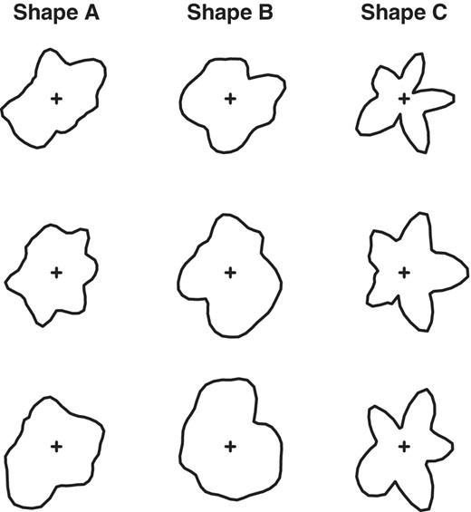
All convex polygons are star-shaped, but the set of star-shaped polygons is substantially larger. Figure 3 shows nine example star-shaped polygons. These examples highlight the variety of polygons that can be star-shaped.
![Rows 1–3: Nine examples of contours enclosing star-shaped polygons with an exponential covariance generated from Gaussian star-shaped contour models (GSCMs) with three different parameter settings, organised by column. The cross sign denotes the starting point, C. Row 4: Estimated probability of a grid box being contained within contours generated by GSCMs with the column's parameters settings. Probabilities estimated from 100 generated contours. The GSCM parameter settings are referred to as (left), (middle) and (right). For all shapes p=50 and κ=2. Values for μ and σ are given in Appendix C. [Colour figure can be viewed at https://dbpia.nl.go.kr]](https://oup.silverchair-cdn.com/oup/backfile/Content_public/Journal/jrsssc/71/5/10.1111_rssc.12592/1/m_rssc_71_5_1688_fig-3.jpeg?Expires=1748949533&Signature=0E2vydEJTakitnO6Pld1MZGFLG81zzgHIuDJMrl1M-gR5NMF9IFoUFc3-RMMYOsxm-lhktO8lCZI8Dc1bVL5lpYwsHGikL-~G-cg-w27Hz7v4isECy7XfIdOC7oqOwNuSYywO0~9IMuJMdq~RC-f4NTfi3pQ~QoAVolupVy4RUz3GG5M7rLKlW3l7dLc4ymJJZ2Ll56jr1bjz8g0WhEHpdV5T07ktdeQ6~3j8o1Swvnvkp7d6tnQ2nUv8UMmqrwmZ8t1Tswj0n-pjITbWuYXJ~BkwtjPGnoVnXseBpDKaGCfTFs89DdJq~BM8mh7gafAmeXfaSTndx-sZeOnA1ssGw__&Key-Pair-Id=APKAIE5G5CRDK6RD3PGA)
Rows 1–3: Nine examples of contours enclosing star-shaped polygons with an exponential covariance generated from Gaussian star-shaped contour models (GSCMs) with three different parameter settings, organised by column. The cross sign denotes the starting point, . Row 4: Estimated probability of a grid box being contained within contours generated by GSCMs with the column's parameters settings. Probabilities estimated from 100 generated contours. The GSCM parameter settings are referred to as (left), (middle) and (right). For all shapes and Values for and are given in Appendix C. [Colour figure can be viewed at https://dbpia.nl.go.kr]
Definition 5Kernel of a star-shaped polygon, : The set of point(s) that satisfy the criterion for in Definition 4 is referred to as the kernel of the polygon, .
Convex polygons are the subset of star-shaped polygons such that .
For any star-shaped polygon, , lines can be drawn from some point, , in the kernel of to all points on a contour, . Assume for the moment that the contour point sequence is unknown, but that the location of is known along with the lengths and directions of the lines from to . Then could be derived from this information with trigonometry. Taking inspiration from this fact, we develop the star-shaped representation. First we define a line set:
Definition 6Line set, : A set of lines, , extending infinitely outward from some starting point at unique angles, , where and are x- and y-coordinates, respectively.
We also define a set of spatial points that produce a star-shaped polygon when connected in order:
Definition 7Star-shaped point set, : A set of spatial points such that
(1)where is a set of distances, is a spatial point, and is a set of unique angles.
A star-shaped point set can be used to represent a contour when the distances are selected systematically:
Definition 8Star-shaped representation, ): Let be a star-shaped polygon and be a starting point. Then, the star-shaped representation of the contour , denoted by , is the star-shaped point set, , where is the set of distances from to the intersection point of the contour line and each line in the line set .
The right panel of Figure 2 shows the components of the star-shaped representation for a sample contour. Let refer to the contour line formed by connecting to for and to for . Let refer to the polygon contained within .
Theorem 1Letwithandfor all. For a star-shaped polygonthere existandsuch thatfor any. (Proof in Appendix A.)
Corollary 1Letdenote the line that extends infinitely outward fromat angleand that intersects. For any, the lineis distinct, that is,for anysuch that. (Proof in Appendix A.)
The star-shaped representation allows for finding how contours differ and what the variability of the contours is in different spatial areas. For example, consider two contours and described with star-shaped representations, and , for common line set . To find how much further one contour extends in any direction, simply find the difference between and where and are the distances from to contours and along a line extending at angle . The variability of the contours along any line is estimated from the variability of the corresponding values in the contours' star-shaped representations.
For a contour enclosing a star-shaped polygon, the star-shaped representation is identical to the point-sequence representation when , , and aligns with the direction of the line segments for all . When these conditions are met, the points are the same for any choice of starting point within the kernel of . However, the angles and lengths will differ depending on .
3 STAR-SHAPED CONTOUR MODEL
3.1 General model
We now propose the star-shaped contour model for generating contours that enclose star-shaped polygons. In later sections, we will build upon this idealised model for star-shaped polygons to develop a model appropriate for ice edge contours that are only approximately star-shaped.
Definition 9Star-shaped contour model, : Let be a fixed starting point, let be a fixed set of unique angles, and let be a probability distribution from which a set of values can be drawn. This set of parameters form a star-shaped probability model if each drawn set can be used to form a corresponding star-shaped points set, , as given in Definition 7.
We now consider a distribution that is appropriate in many circumstances. We assume that follows a Gaussian distribution,
where is a mean vector and the parameter is a positive-definite covariance function. We further assume that and are such that mass on non-positive is negligible. (In practice, if in a small proportion of cases, a generated is non-positive, its value can be set to some small .) We call this model the GSCM. The GSCM can be seen as a finite approximation to the planar version of Gaussian Random Particles proposed in Hansen et al. (2015). GSCMs can produce a fairly flexible set of contours. The first three rows in Figure 3 illustrate some types of contours GSCMs can produce.
Because of how is constructed, reasonable and that align with typical observable values will avoid substantial non-positive . The values represent distances from a starting point , so are automatically non-negative. Some points in the kernel of the polygon will typically be centrally located points. Lengths close to zero can be avoided by using one of these points for .
Covariance matrices, , are based on the structure of the lines in the line set. The correlation structure for the set of distances, , is a function of the angles, , of the lines in the line set. Covariances based on angles are complicated by the fact that 0 and represent the same angle. So, the difference between two angles does not necessarily correspond to how far apart the angles actually are. Specialised covariance functions have been derived that remain valid when distances are indexed by angle (Gneiting, 2013). Denote the angle between and by .
Typically, the correlation between and will decrease as increases. For the simulation examples in this paper, we focus on an exponential covariance structure, where and . The element, , in the ith row and jth column of this covariance is
Different parametric covariance structures give different forms for how the correlation between and decreases as . For an exponential covariance, the parameter controls how rapidly the contour can change over space, that is, the roughness or smoothness of the contour. For example, Figure 4 shows sample contours with the same and values as in Figure 3. However, the contours appear smoother because of the different covariance structure. The resolution of the data should also be considered in considering the roughness of the contour. If the data resolution is high, information about how smooth or rough the contours are can be assessed and modelled accurately with the selection. If the resolution is low, though, only smoother contours will be possible, and must be restricted accordingly. In other words, estimates of from data may be limited by the data's resolution.
Rows 1–3: Nine examples of contours enclosing star-shaped polygons with a multi-quadric covariance generated from Gaussian star-shaped contour models (GSCMs) with three different parameter settings, organised by column. The cross sign denotes the starting point, . The GSCM parameter settings are referred to as (left), (middle) and (right). For all shapes , and Values for and are given in Appendix C.
3.2 Fitting GSCMs
We now turn to building a GSCM given observed contours. We assume that the data are observed contours, , that enclose regions that are star-shaped polygons. (Note that each may be derived from binary grid as described in Section 2.) We also assume that the contours are generated from a common, but unknown, and , that is, and . We first find a starting point, , and angles, . Then, we estimate and the parameters controlling based on the observed for the selected and angles .
3.2.1 Fixing the starting point and the set of angles
The accuracy of the GSCM depends on the selection of and . If is selected outside the kernel of the polygons, the line set will not be able to intersect with all sections of the contour line. So some area within the true enclosed contour will be missed by the contour model. Similarly, if is not dense enough, some direction changes in the contour will not be modelled. The influence of the density of will be greater if the contour changes direction rapidly. The set of angles, , is selected to keep the mean difference in area between the observed contours' enclosed polygons and the star-shaped representations of these contours' enclosed polygons below some value.
Following Corollary 1, any set of distinct angles can be used to form a star-shaped representation of a contour. We recommend using evenly-spaced angles. Figure 5 illustrates how a star-shaped contour is approximated with a star-shaped representation with evenly-spaced . Using evenly spaced angles ensures that the model represents all sections of the contours with the same level of precision. While some sections of the contours may change more rapidly than others and require more lines to represent well, exactly where these changes occur is hard to determine without having already modelled the contour. Therefore it is easier to select a density of lines to use consistently for all sections of the contour.
![Components of a contour represented by a point-sequence representation (left) and a star-shaped representation approximating the point sequence with evenly spaced angles (right) [Colour figure can be viewed at https://dbpia.nl.go.kr]](https://oup.silverchair-cdn.com/oup/backfile/Content_public/Journal/jrsssc/71/5/10.1111_rssc.12592/1/m_rssc_71_5_1688_fig-5.jpeg?Expires=1748949533&Signature=u13Xgstq~5296hlo11pj6komD4Yswz-9XpzUFvuzdHefoHjiG~4ZoDQLjqzfEv~Z69sWH5XmoS2~jyeSKaIgUs3eYxGEyib1m33GUXooX~Zhg8nGeCDsCV~VK1Q14HToe8y6LMwRrvSqMZKk~EdDoxIGHZjLmGaj9sZ3kydUJiEIBGqWCQu9ZKiLNdp~kfzc2a65Fny3~X5x2nl3bcgGumdvluYD74sbcAI5ViH9urnOY4RAxJ5wIA9d9ioUGYxcxiY0kVHugqHl706vnzEm5599xkwLtmKP-cZ3ztQZFny6YhT-NMiI6dy1jeccBQQRwslQQdxNk9Pdn5UgXBZy7A__&Key-Pair-Id=APKAIE5G5CRDK6RD3PGA)
Components of a contour represented by a point-sequence representation (left) and a star-shaped representation approximating the point sequence with evenly spaced angles (right) [Colour figure can be viewed at https://dbpia.nl.go.kr]
This sensitivity of GSCMs to the choice of and motivates the development of a careful procedure to select them. Our procedure seeks to minimise the area that cannot be represented by the GSCM while balancing computational constraints. We fix a starting point, , and set of angles, , that can be used to describe the observed contours accurately. We first describe how to find conditional on and conditional on separately. Then, we describe an iterative algorithm to fix both values together.
Findingconditional on: The starting point used in modelling is selected to minimise the difference in area between the observed contours' enclosed polygons and the star-shaped representations of the observed contours' enclosed polygons. Conditional on , we define the set that differs between an observed polygon, , and a star-shaped representation of that contour with starting point, , as
where the superscript denotes the complement of the set. The area contained within this set is denoted by . The lower this area, the more accurately the GSCM will be able to represent the enclosed polygons. So, selecting a such that for all would be optimal. Assuming is known, Theorem 1 guarantees that at least one point exists where for all . If only one point satisfies this condition, then . However, any location for which is approximately zero will be able to represent the area within the contour well. As such, we select numerically with
where is the mean function and is a grid of points. The finer the grid of the closer will be to zero. The number of points in can be reduced by restricting assessment to the kernels of star-shaped polygons.
Theorem 2Letbe a set ofstar-shaped polygons, letbe the true starting point, and letdenote the intersection of the kernels of all polygons. Then,. (Proof in Appendix A.)
Therefore, we need only perform the optimisation in Equation (5) for . Algorithms for computing are given in Appendix B.
Findingconditional on: As motivated in Section 3.2.1, GSCMs can be fit with evenly spaced angles. So, finding the set of angles only requires finding , the number of elements in .
Since controls the dimensions of and , larger requires more computation. We then identify the approximately lowest that keeps the mean difference in area below some value. To allow comparisons of polygons of different sizes, we often express this allowable mean difference in area as a proportion, , of the average area of the polygons. This constraint on the allowable differing area is then
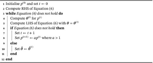
where is the mean function and denotes the area of the polygon . We use Algorithm 1 to find an approximately minimal that satisfies the constraint in Equation (6). To avoid selecting a larger than necessary, should generally be initialised such that Equation (6) is not satisfied. Smaller values of will make more precise, but will require more computation than larger . Using lower values of will generally result in higher and lower differences in area. Section 5.3 uses simulation to explore different .
Finding conditional on C
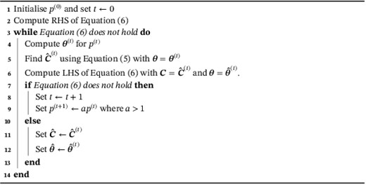
Findingand: In practice, neither nor will be known. So, to find both values, we iterate between setting conditional on and conditional on . Algorithm 2 describes this process. As in Algorithm 1, the initial value, , should be selected to be low enough that Equation (6) is not satisfied. Otherwise, we may select a larger than is needed. Smaller values of will result in more precise determination of , but will require more computation.
Finding and
3.2.2 Computing a posterior
Once and are determined, model fitting is straightforward. For each observed contour, the observed values are computed given and . Then from Equation (2), the corresponding likelihood for these is just that of a multivariate normal distribution:
Estimates of the mean vector and the parameters controlling can be estimated using any standard method.
For demonstration purposes in the simulations and for modelling the sea ice edge we take a Bayesian approach. We assume an exponential covariance as in Equation (3) with parameters and . We use the following simple prior distributions for , and . We assume a multivariate normal prior distribution for :
The hyperparameters and give the mean and covariance of the prior distribution. For the example exponential covariance defined in Equation (3) we assume uniform priors on and :
where the hyperparameters and are upper bounds. Samples from the posterior distributions of the parameter can be found via standard Markov chain Monte Carlo (MCMC).
3.2.3 Estimating gridded probabilities and credible intervals
Sampled contours can be used to estimate the probability of a given area being contained within a contour. Consider sample contours, . Each generated contour can be approximated by a binary grid, , of dimension . Let indicate the grid box in the ith row and jth column of . Let indicate whether the majority of the area in grid box is inside or outside contour . Most grid boxes will be entirely inside or outside the contour; however, grid boxes that intersect the generated contour will contain area both inside and outside the contour. Ideally, the grid selected should be fine enough to ensure that little area is contained within these transitional grid boxes. Averaging the binary grids produces an matrix, , with elements , that indicate the probability of grid box being contained within a contour. The last row of Figure 3 shows estimated gridded probabilities obtained from generated contours from the corresponding GSCMs.
Credible regions for the location of the contour can be computed from . The credible region, , is formed from a union of grid boxes that satisfy the condition
3.2.4 Rescaling data
For numerical convenience in fitting and generating contours, it is often desirable for all contours to be contained within the unit square. Observed data will typically need to be rescaled to be within these bounds. Data should be re-scaled such that generated contours do not extend outside the unit square. A good re-scaling also ensures that the contours that will be generated rarely, if ever, extend outside the unit square.
Therefore, we re-scale observed contours to be within an square. This re-scaling provides a buffer region of width on the outside of the unit square in which no contours have been observed. Therefore, if generated contours extend farther than the observed contours, they will typically go into this buffer region rather than outside the unit square. The higher the variability of contours, the larger the value of needed to avoid generating contours that go beyond the unit square.
To transform a set of observed coordinates, , to the square of dimension , let and denote the minimum and maximum observed -coordinates from all spatial points in all contours in . Define and analogously for the -coordinates. Let and let denote the ith point in the jth.
Then for all and all , we shift and re-scale all coordinates for observed points with the transformation
Note that Equations (12) and (13) adjust the coordinates such that all lengths 's are re-scaled by the same constant and so still follow a Gaussian distribution.
4 COVERAGE METRIC
To assess if our probabilistic contour model performs well in representing the ice edge, a metric is needed. A good model correctly identifies the region where the contour could plausibly be located. So we focus on the coverage of prediction intervals for star-shaped contours. With an accurate contour model, the variability of the generated contour would be correctly represented along all parts of the contour. In designing an appropriate metric, we leverage the star-shaped structure of the data. The general idea is to assess coverage for each line in a line set individually.
To make this idea precise, we define several quantities illustrated in Figure 6. As in Equation (11), let be the credible region obtained from some contour model. Define some test line set with evenly spaced lines. Define as the line segment formed from the intersection of the credible region and the line . We refer to as a test line. Also, define as the intersection of some observed contour and line . Note that will always be a single point when the polygon is exactly star-shaped and .
![Illustration of coverage assessment for a contour line, S‾i (red), and a 1−α credible region, I1−α (light blue). The line segments, I1−α,k, corresponding to the intersection of the I1−α credible region and line ℓk are coloured black when they cover Si,k and blue otherwise. The centre of the star-shaped polygon from which the contour is generated is denoted by a green cross sign. The line set ℒ∗(C∗,θ∗) contains 100 line segments evenly spaced by angle. [Colour figure can be viewed at https://dbpia.nl.go.kr]](https://oup.silverchair-cdn.com/oup/backfile/Content_public/Journal/jrsssc/71/5/10.1111_rssc.12592/1/m_rssc_71_5_1688_fig-6.jpeg?Expires=1748949533&Signature=aumJJzvW65ZTiXt6rI7c7EYQ3l~GePxe4L966pRTK-axBd5658kMa-DmsZIYd-WOQu75ZJfSImYpdJmO4PWNwA0nvVhUuYEC~FkD0NWCigfSUc0LmQwm-PDT7XI~k~E3kIum5A0HxK3OQ01apDwR2MtkLbU1zRP9Bto2vUmKWqlLYR7IfsJVqdGEurxH0r6yHeO8ICZzf5vZ3vNbLlaIqvB3-mFwTIqx9d97CLEz4AV-ZiOgGMVBJ00527F9JGp4XwtonhlK0dj9RhXVyYFfq~rfKjyOrHbQTM952AV4pBPwrn33rOVsEKplItT1hwSnSPWGRPFJF2amKkklfTAJSA__&Key-Pair-Id=APKAIE5G5CRDK6RD3PGA)
Illustration of coverage assessment for a contour line, (red), and a credible region, (light blue). The line segments, , corresponding to the intersection of the credible region and line are coloured black when they cover and blue otherwise. The centre of the star-shaped polygon from which the contour is generated is denoted by a green cross sign. The line set contains 100 line segments evenly spaced by angle. [Colour figure can be viewed at https://dbpia.nl.go.kr]
Let indicate whether the intersection points of the observed contour and the line are contained within the intersection of the credible region and line . Then, for credible intervals with perfect coverage, for any ,
In other words, the part of the true contour that intersects line is contained within the credible contour region along line with probability .
We consider coverage behaviour for a set of observed contours, that enclose star-shaped polygons assumed to have been generated from the same model. Each is assumed to be independent of for all .
For a credible interval with perfect coverage for any , ,
for sufficiently large sample size, . This equation is used to assess coverage in practice. Equation (15) not holding for any indicates the variability of the contour on test line is not correctly represented by the credible region.
With this set-up, and are independent for all conditional on the parameters of the GSCM. So for a given line ,
Since the distributional behaviour of the quantity is known, the expected variability of the mean coverage given a particular sample size is known. This information can be accounted for in a simulation study or cross-validation experiment.
We also consider how coverage on one test line in relates to coverage on another test line. The location of points on a contour are generally correlated. So, and are correlated. Typically and will be more correlated the smaller the angle distance from and . What this means is that while
is fixed and known, the quantity is not a good metric to assess to coverage. The distribution of depends on the correlation structure of the points on the contour. For a contour with high correlation among points, the quantity will be substantially affected by what contour happens to be sampled. For intuition, consider a contour with high correlation among all . In this case, the contour is likely to be entirely within the credible interval or entirely outside of it. So, will be either 0 or M.
These relationships among coverage for and show that sample sizes need to be considered in terms of the number of contours observed. The metric should be considered for all elements in . The number of test lines, , should be set such that accuracy is assessed with detail appropriate for the application. Since the true exact value of , is unknown, we cannot simply set . However, based on the observed data, we should have a general idea of . So, we set , to ensure that . We also evenly space with . By assessing coverage on a substantially greater number of test lines than the true number of lines, we ensure that coverage is at least assessed near every true line.
To carry out this assessment, a fixed starting point and should be selected. In simulation studies, the true value of will be known and we can let . For assessment of real data such as in a cross-validation study, a starting point for will be unknown and must be determined. We recommend using a that minimises the difference in area between the observed contours' enclosed polygons and the star-shaped representations of the observed contours' enclosed polygons as in Section 3.2.1, that is, let .
This assessment approach differs from how contours have been assessed in the context of level exceedances. There, a credible region or confidence region has often been defined as the region that covers the true contour in its entirety -proportion of the time (e.g., Bolin & Lindgren, 2015; French, 2014). With credible (confidence) regions constructed to satisfy this definition, coverage can be assessed by determining what proportion of the time the true contour is fully contained within the region. We opt not to use this metric since our goal is to develop a method to generate ice edge contours directly. Correlation along the contour makes assessing the probability of capturing the entire contour difficult. Our metric reflects that we are most concerned with getting the right variability in all parts of the contour. We are less concerned with identifying a larger area that contains that entirety of the contour with high probability. Our intervals are therefore narrower than would be required for these global intervals.
5 SIMULATION STUDIES
5.1 Simulation details
Before evaluating the ice edge data, we consider how the star-shaped model performs in inferring distributions of simulated data. We consider performance with varying numbers of observations, different constraints for the allowable mean difference in area ( as defined in Section 3.2.1), and varied GSCM parameters.
In many of our simulations, we focus on a particular GSCM with that we will refer to as Shape A. The correlation structure of follows the exponential form given in Equation (3). The vector of mean distances, , and variance parameter vector, , change gradually. The exact values of and can be found in Appendix C. Unless otherwise noted, is set to 2. Example generated contours and gridded probability estimates for Shape A are given in the left panel of Figure 3.
The values and are found as described in Section 3.2. The parameter values are fit from observations using MCMC. Chains are run for 50,000 iterations with the first 15,000 iterations discarded as burn-in. The prior parameters are , , , and where is a diagonal matrix of dimension by . The value refers to the number of angles in .
For all simulations, we use 40 evaluation runs. On each evaluation run, we estimate the GSCM parameters using contours generated from the true GSCM as training data. From the resulting fitted GSCM, we generate 100 contours and find credible intervals as described in Section 3.2.3. To evaluate coverage, we compare the credible interval with a single ‘true’ contour drawn from the true GSCM. We record the coverage for a set of evenly spaced test lines with as described in Section 4. We report the mean coverage over the 40 evaluations and the SD across the test lines.
5.2 Varying number of observations,
Our first simulation varies , the number of simulated ‘observed’ contours used to fit the Shape A GSCM. We consider coverage performance for 10, 20 and 50 simulated observed contours with . Table 1 displays the results of this simulation.
Mean coverage values for 40 simulations of fitting the contour distribution for with different number of observed contours sampled as training data
| Nominal | N = 10 | N = 20 | N = 50 |
|---|---|---|---|
| 0.80 | 0.87 (0.04) | 0.79 (0.07) | 0.76 (0.06) |
| 0.90 | 0.94 (0.04) | 0.89 (0.05) | 0.86 (0.05) |
| 0.95 | 0.98 (0.02) | 0.95 (0.03) | 0.93 (0.04) |
| Nominal | N = 10 | N = 20 | N = 50 |
|---|---|---|---|
| 0.80 | 0.87 (0.04) | 0.79 (0.07) | 0.76 (0.06) |
| 0.90 | 0.94 (0.04) | 0.89 (0.05) | 0.86 (0.05) |
| 0.95 | 0.98 (0.02) | 0.95 (0.03) | 0.93 (0.04) |
Notes: In each simulation, evenly spaced test lines were evaluated with . SDs across the test lines are given in parentheses. Priors and Markov chain Monte Carlo details are given in Section 5.1.
We find that coverage improves for compared to . We find slightly worse performance for than , although the performances are not substantially different given that we had only 40 evaluation runs. These results indicate that obtaining some minimum sample size is important for coverage performance. For small sample sizes, on the order of , the data alone may not be enough to produce accurate coverage, particularly for the 80 credible interval. However, data sets of this size can potentially still be modelled correctly if informative priors can supplement the observations.
5.3 Varying allowable difference in area,
In these simulations, we evaluate how coverage accuracy is affected by the parameter introduced in Section 3.2.1. This parameter controls the allowable differing area when setting the number of lines used in fitting, , and how accurate must be. We evaluate coverage for Shape A with set to and 0.01. These selections set the allowable mean difference in area to 3, and of the mean area contained within the observed contours. We also consider how correlation in affects the need for different by evaluating each for three different values: 1, 2 and 4. Table 2 displays the mean coverage across test lines for three -levels along with the mean found. On each evaluation the number of sampled contours is set to .
Mean coverage values for 40 simulations fitting the contour distribution for with different values of
| Nominal | Coverage | Mean | Coverage | Mean | Coverage | Mean | |
|---|---|---|---|---|---|---|---|
| 1 | 0.8 | 0.86 (0.05) | 38.48 (0.8) | 0.87 (0.06) | 45.65 (1.8) | 0.86 (0.05) | 55.20 (9.2) |
| 0.9 | 0.94 (0.04) | ” | 0.94 (0.04) | ” | 0.94 (0.03) | ” | |
| 0.95 | 0.98 (0.02) | ” | 0.98 (0.02) | ” | 0.98 (0.02) | ” | |
| 2 | 0.8 | 0.82 (0.05) | 32.65 (0.9) | 0.80 (0.06) | 41.27 (1.2) | 0.84 (0.06) | 50.50 (1.9) |
| 0.9 | 0.92 (0.04) | ” | 0.90 (0.05) | ” | 0.91 (0.04) | ” | |
| 0.95 | 0.96 (0.03) | ” | 0.95 (0.04) | ” | 0.95 (0.03) | ” | |
| 4 | 0.8 | 0.86 (0.06) | 28.38 (0.67) | 0.79 (0.05) | 36.67 (0.9) | 0.80 (0.07) | 48.45 (1.0) |
| 0.90 | 0.93 (0.04) | ” | 0.89 (0.04) | ” | 0.91 (0.04) | ” | |
| 0.95 | 0.97 (0.03) | ” | 0.94 (0.03) | ” | 0.97 (0.02) | ” | |
Notes: In each simulation, 20 observed contours were sampled as training data and evenly-spaced test lines with were evaluated. SDs across the test lines are given in parentheses. The mean is given for each along with the SD across the evaluation runs in parentheses. Apostrophes indicate that the entry is the same as the line above it. Priors and Markov chain Monte Carlo details are given in Section 5.1.
We find that the mean coverage accuracy is only modestly affected by the value of . These results support the idea that using a lower in many cases will reduce computation while not reducing model performance. We also find that, for a given , an increase in corresponds to a decrease in . In other words, for a contour with higher correlation among , a smaller set of lines can adequately represent the contour distribution.
5.4 Varying GSCM parameters
We also evaluate contour models that have mean values, , that vary more slowly and more quickly than in Shape A. These GSCMs are denoted as Shape B and Shape C, respectively. Figure 3 shows sample contours and probability distributions for these shapes. Both models are defined to have and Exact values for and for Shape B and Shape C can be found in Appendix C. We report coverage results in Table 3 for three -levels using simulated observed samples and .
Mean coverage values for 40 simulations fitting the contour distribution for Shapes A, B and C
| Nominal | Shape A | Shape B | Shape C |
|---|---|---|---|
| 0.8 | 0.79 (0.07) | 0.79 (0.06) | 0.87 (0.05) |
| 0.9 | 0.89 (0.05) | 0.89 (0.05) | 0.95 (0.03) |
| 0.95 | 0.95 (0.03) | 0.95 (0.04) | 0.98 (0.02) |
| Nominal | Shape A | Shape B | Shape C |
|---|---|---|---|
| 0.8 | 0.79 (0.07) | 0.79 (0.06) | 0.87 (0.05) |
| 0.9 | 0.89 (0.05) | 0.89 (0.05) | 0.95 (0.03) |
| 0.95 | 0.95 (0.03) | 0.95 (0.04) | 0.98 (0.02) |
Notes: In each simulation, simulated observed contours were sampled as training data and evenly-spaced test lines were evaluated with . SDs across the test lines are given in parentheses. Priors and Markov chain Monte Carlo details are given in Section 5.1.
We find reasonably accurate coverage performance for all three shapes. The method performs slightly worse for Shape C than for Shape A and Shape B. This performance difference is likely due to the difficulty of getting the pointed sections of Shape A in the correct location if is even slightly underestimated. This result indicates that for contours that look like Shape A, lower values may be appropriate. We note that the simulations in this section are relatively symmetric. Results might be more variable moving around the contours if there was less symmetry. In such cases a lower would be appropriate to account for this heterogeneity. Overall, the good performance across parameter settings indicates that a range of contours can be well approximated by a GSCM.
6 MODELLING CONTOURS ENCLOSING APPROXIMATELY STAR-SHAPED POLYGONS
The ice edge contours enclose polygons that are approximately, but not exactly, star-shaped. This section describes how to assess whether the GSCM is appropriate given the observed data, and how the fitting procedure is altered if the observed contours enclose polygons that are not exactly star-shaped.
6.1 Assessing appropriateness of GSCM
Two main assumptions must be met to apply the GSCM: the polygons enclosed by the contours must be approximately star-shaped and all contours should have at least one common point. The latter assumption is needed to define a starting point and can be trivially assessed. The former assumption can be assessed using metrics that describe how close an observed contour is to enclosing a polygon that is star-shaped. These metrics focus on the difference in the area between the polygon enclosed by the true contour and the polygon enclosed by the star-shaped representation of the contour. If these differences are small for a set of observed contours, , then the GSCM can be applied.
We relax Definition 8 to make precise how to approximate an arbitrary polygon with a star-shaped representation. Two main differences between star-shaped polygons and arbitrary polygons are addressed in these new definitions: (1) an arbitrary polygon may not have a kernel and (2) the contour line enclosing an arbitrary polygon may intersect with some of the lines in the line set multiple times. The new star-shaped representation definitions are:
Definition 10Underestimated star-shaped representation, : Let be a polygon described by ordered spatial points , let be a starting point, let be an arbitrary set of unique angles, and let be a set of distances from to the closest intersection point of the contour line and each line in the line set . Then, the star-shaped representation of the contour, , is the underestimated star-shaped representation, .
Definition 11Overestimated star-shaped representation, : Let be a polygon described by ordered spatial points , let be a starting point, let be an arbitrary set of unique angles, and let be the set of distances from to the farthest intersection point of the contour line and each line in the line set . Then, the star-shaped representation of the contour, , is the overestimated star-shaped representation, .
The names of these representations highlight that these polygons generally under- or overestimate the area contained within the true polygon. For contours that enclose star-shaped polygons, if , only one intersection is found between the contour line and all lines in the line set. So, . For notational convenience, let and . Then the sets that differ between the true contour and the under- and overestimated star-shaped representations are
where the superscript denotes the complement of the set. Let and be the area contained within these sets. Figure 7 illustrates the quantities described in this section for four contours. The difference in area is zero only if the polygons are star-shaped. More precisely:
![Four contours (left) with their underestimated star-shaped approximations, V˜u(C^u,θ,S), (red, centre), and their overestimated star-shaped approximations, V˜o(C^o,θ,S) (blue, right). The polygon in the top row is star-shaped, and the other three polygons are not. Pink and blue sections in the centre and right panel show the respective differing areas, Au(C^u,θ,S) and Ao(C^o,θ,S). The red crosses in the central panel and the blue crosses in the right panel denote the estimated starting points, C^u and C^o. The vector θ contains 200 elements spaced evenly in the interval [0,2π]. [Colour figure can be viewed at https://dbpia.nl.go.kr]](https://oup.silverchair-cdn.com/oup/backfile/Content_public/Journal/jrsssc/71/5/10.1111_rssc.12592/1/m_rssc_71_5_1688_fig-7.jpeg?Expires=1748949533&Signature=TyGZmgzRz0MM3~L9OY4c7OkBiKEe-bS~jOxdKO5T3lMnJ3wgZ5I07S4KjuyBnnZp6qocTjvq5aRG4Jz8y2b~SucMBmQ~EOh5hGNeEGM-NO5HI-rQhReCXDT5RozFdJl3lrbHgEbj8BOTfldOXwH239J1Nv9RX7XZR~D1usd7MPqBmvnJR0NW7uANkQ3BXTRP99NeQl6wT1HRa4rXBFiubOFRWLzvseR~K3vbfktdNJFEnxeNrdU-ysx60aodx97DDnVXYS~~92f8mScPOFVx8e~F1Temr9Zh9-MZ-mmeVlYZGFkvIG2XIqL9ujtd6IzaOytl~CADdSd21RKsWHt1LA__&Key-Pair-Id=APKAIE5G5CRDK6RD3PGA)
Four contours (left) with their underestimated star-shaped approximations, , (red, centre), and their overestimated star-shaped approximations, (blue, right). The polygon in the top row is star-shaped, and the other three polygons are not. Pink and blue sections in the centre and right panel show the respective differing areas, and . The red crosses in the central panel and the blue crosses in the right panel denote the estimated starting points, and . The vector contains 200 elements spaced evenly in the interval . [Colour figure can be viewed at https://dbpia.nl.go.kr]
Theorem 3For any polygonthat is not star-shapedandfor anyand. (Proof in Appendix A.)
For easier comparison of these differences in area across sets of polygons of different sizes, these areas can be expressed as percentages of the mean total area of the polygons. Table 4 reports the difference in area for the contours in Figure 7, and their star-shaped representations as a percentage of the total area of the polygon.
The differing area for the under- and overestimated star-shaped approximations, and , for the contours in Figure 7
| Underestimated | Overestimated | |
|---|---|---|
| Contour 1 | 0.00 | 0.00 |
| Contour 2 | 0.43 | 0.24 |
| Contour 3 | 4.44 | 9.78 |
| Contour 4 | 15.65 | 8.46 |
| Underestimated | Overestimated | |
|---|---|---|
| Contour 1 | 0.00 | 0.00 |
| Contour 2 | 0.43 | 0.24 |
| Contour 3 | 4.44 | 9.78 |
| Contour 4 | 15.65 | 8.46 |
Notes: Differences in area are computed numerically and expressed as a percentage of the total area of the polygon. The vector contains 200 elements spaced evenly in the interval .
6.2 Fitting GSCMs to approximately star-shaped polygons
The approach to fitting in Section 3.2 needs to be altered slightly for contours that enclose regions that are only approximately star-shaped contours. The values of need to be computed using the under- or overestimated star-shaped approximation as given in Definitions 10 and 11. Whether to use the under- or overestimated star-shaped representation depends on the application. In some cases, asymmetric risks may motivate selecting a model that generally over- or underestimates the area within the polygon. Otherwise, both and can be computed for the set of observed contours and whichever representation results in less difference in area can be selected. Fitting the posterior proceeds as in Section 3.2.2. Finding probabilities and credible intervals proceeds as in Section 3.2.3.
We find and using nearly the same algorithm as in Section 3.2.1, except that we update the star-shaped representation in Equations (5) and (6) to be the under- or overestimated star-shaped representation. Specifically, we replace Equation (5) with
for the underestimated representation and
for the overestimated representation. The values and denote the estimated starting points for the two approximations, respectively. As before, is the mean function. Like in Section 3.2.1, we evaluate these functions of the area difference at a grid of possible locations, . Unlike in Section 3.2.1 we cannot use the estimated intersection kernel to reduce the size of , since the polygons are not exactly star-shaped. However, we note that the starting point must be common to all observed polygons, so we constrain to only cover areas in the intersection of all observed polygons, . Equation (6) is also slightly changed so that
for the underestimated representation and
for the overestimated representation. The value still represents the mean function and is still a proportion.
6.3 Coverage metric for approximately star-shaped polygons
This metric introduced in Section 6.1 is essentially the same when applied to approximately star-shaped polygons. However, , the intersection of an observed contour and line , may now contain multiple points since polygon is only approximately star-shaped. A single point of intersection will still be more common when polygons are approximately star-shaped. Aside from this change, the definition of remains the same when is composed of multiple points. So, all subsequent definitions and properties in Section 6.1 hold as well.
6.4 Simulation study of contours enclosing approximately star-shaped polygons
In these simulations, we assess GSCM performance for contours that enclose polygons that are only approximately star-shaped. We simulate contours that vary systematically in how much the polygons they enclose differ from being star-shaped. Figure 8 shows examples of the types of contours we will evaluate.

Three generated contours that enclose polygons that are only approximately star-shaped. From left to right, contours have increasing area that cannot be described with a star-shaped representation.
To obtain these contours, we first generate polygons that are star-shaped from a GSCM. We then append sections to these polygons that cause the polygons to no longer be star-shaped. The appended sections loop back around the outside of the initial polygon over some number of lines in the initial line set. The number of initial lines looped back over are selected randomly from some uniform distribution. Appended sections that loop around a larger number of lines are longer than appended sections that loop over a smaller number of lines. Longer appended sections result in more area that cannot be described with a star-shaped representation than shorter appended sections. How close the appended section is to the initial star-shaped polygon and the width of the appended section are selected randomly from uniform distributions.
We consider 40 evaluation runs for three different uniform distributions for the number of initial lines that the appended section loops back over. The initial GSCM is set to be Shape A with and . In each evaluation run, the GSCM is fit to simulated contours. Rather than fixing to determine and in these simulations, we set . We then estimate conditional on . This choice simplifies the interpretation of our results. (Larger 's would be needed as the area differing from a star-shaped polygon increases. So, it would be difficult to distinguish whether performance differences were due to changes in or changes in how close to star-shaped the polygons are.) We initially run these simulations using a random location for the appended section and then repeat these simulations with a fixed location for the appended section. Results are reported in Table 5.
Mean coverage values for 40 simulations of fitting the contour distribution for approximately star-shaped data
| Nominal | Unif | Unif(2, 3) | Unif | |
|---|---|---|---|---|
| Random location | 0.8 | 0.90 (0.04) | 0.88 (0.07) | 0.90 (0.05) |
| 0.9 | 0.96 (0.02) | 0.94 (0.04) | 0.93 (0.04) | |
| 0.95 | 0.98 (0.02) | 0.97 (0.02) | 0.95 (0.03) | |
| Fixed location | 0.8 | 0.79 (0.08) | 0.77 (0.12) | 0.77 (0.16) |
| 0.9 | 0.88 (0.06) | 0.87 (0.10) | 0.87 (0.15) | |
| 0.95 | 0.94 (0.04) | 0.93 (0.07) | 0.93 (0.13) |
Notes: The number of initial lines for the appended section to loop back over are selected randomly from a Uniform(a, b) distribution. In each simulation, simulated observed contours were sampled as training data and evenly spaced test lines with were evaluated. The appended sections are located in a random position in the first three cases and a fixed location in the second three cases. SDs across the test lines are given in parentheses. Priors and Markov chain Monte Carlo details are given in Section 5.1.
With a random location for the appended section, we find that applying GSCMs still results in reasonable coverage for the 90 and credible intervals. For the credible interval, performance is moderately degraded. Interestingly, average performance does not seem to be correlated with how large the appended section to the contour is. When an appended section is added to a fixed location, we find that the mean coverage across the test lines is relatively accurate; however, the SD is quite high, suggesting that coverage is actually poor in some parts of the contours. Figure 9 illustrates this variability in performance for the case with the number of initial lines looped over distributed Uniform(4, 5). We plot the proportion of evaluation runs covered by the credible intervals for each test line individually.
![Proportion of lines covered out of 40 evaluation runs plotted against the index of each of M=100 evenly spaced test lines for the 90% credible interval for the contours enclosing approximately star-shaped polygons. The black line corresponds to when the appended sections are added to a random location and the blue lines corresponds to when the appended sections are added to a fixed location. The number of initial lines looped back over are selected randomly from a Uniform (4, 5) distribution. Nominal coverage is in red. Priors and Markov chain Monte Carlo details are given in Section 5.1. [Colour figure can be viewed at https://dbpia.nl.go.kr]](https://oup.silverchair-cdn.com/oup/backfile/Content_public/Journal/jrsssc/71/5/10.1111_rssc.12592/1/m_rssc_71_5_1688_fig-9.jpeg?Expires=1748949533&Signature=fVTYrmb1shdvFN10AggbXrhL1rnzDccP8Zc-rR7RfaEtfUIizpDDBfDRsbFLH9DTG~XKc6ocNdFPX3pOPLYmR~A8QObRj-EhA9COxwOSev8MnTGFXmGAjVrTm0~Yh7lWiDv-mzLYKKbFM-4YRHAim-cqw0BC-dgGc~fDRHn7cYkM2Yu~dt1Ok-b~-P5rvPW6u~FAqQjtYZ7LHUodPtHHovzeqT7EuAg0KlKx4KLxg9f-Hi8CqdaWi21EcHvesNfwZuTvCvV9zxb62Yq4KnN5TDaZ5P22964KEPZmwkcHk-EMJEoA8eAaU71ENmC-OPY0Vy6l5JPMYqylngBnnQjeBQ__&Key-Pair-Id=APKAIE5G5CRDK6RD3PGA)
Proportion of lines covered out of 40 evaluation runs plotted against the index of each of evenly spaced test lines for the 90 credible interval for the contours enclosing approximately star-shaped polygons. The black line corresponds to when the appended sections are added to a random location and the blue lines corresponds to when the appended sections are added to a fixed location. The number of initial lines looped back over are selected randomly from a Uniform (4, 5) distribution. Nominal coverage is in red. Priors and Markov chain Monte Carlo details are given in Section 5.1. [Colour figure can be viewed at https://dbpia.nl.go.kr]
The location of the fixed appended section is under-covered. In contrast, no obvious patterns are seen when the location of the appended section is random. These results indicate that contours that enclose polygons that modestly differ from star-shaped contours can be modelled with GSCMs. However, if areas differing from the star-shaped representation occur in the same location repeatedly, additional modelling of these areas may be needed to avoid systematic errors in coverage.
7 APPLYING GSCMS TO THE ARCTIC SEA ICE EDGE CONTOUR
We now illustrate how GSCMs can be used to model the Arctic sea ice edge. We focus on the ice edge in September, the month when the ice-covered area in the Arctic is at its annual minimum. September holds particular interest for maritime planning, since vessel traffic is typically highest when there is the least sea ice.
We focus on modelling the sea ice edge over a short set of recent years. These types of models can be used to make statements about how probable sea ice edges will be in the near future and/or to describe plausible sea ice edges that align with the oceanic and meteorological conditions in this time period. The GSCM can be applied to generate plausible sea ice edge contours and corresponding credible intervals for the ice edge contour. Note that with climate change, the Arctic area covered by sea ice (Comiso et al., 2008; Stroeve et al., 2012) has reduced on average over time. So, observed ice edge contours from decades past are not similar to ice edges observed recently. However, on short time scales, the change in average meteorological and oceanic conditions is small. So, assuming that each observed September sea ice edge is an independent draw from a stationary distribution is appropriate. Additionally, the correlation of sea ice from 1 month to the next decays rapidly, so observations from one year apart can be treated as independent.
The data used in fitting a sea ice edge model is a monthly average observational product produced by the National Aeronautics and Space Administration satellites Nimbus-7 SMMR and DMSP SSM/I-SSMIS and downloaded from the National Snow and Ice Data Center (Comiso, 2017). The data are composed of gridded fields reporting the sea ice concentration, or percent of ice-covered area in each grid box. Following a convention used by sea ice researchers, grid boxes with at least 15 concentration are treated as containing sea ice and grid boxes with less than 15 concentration are treated as open water. This thresholding is needed because satellite estimates for very low concentrations are not considered reliable. The transition from complete sea ice cover to open water occurs over a narrow spatial range, so the ice edge is not particularly sensitive to the exact threshold selected. Each month's gridded field is converted to an ordered sequence of points as described in Section 2. We refer to the ordered sequences of points associated with each month of data as the observed ice edge in that month.
To assess the sea ice edges generated by the GSCM, we perform a leave-one-out cross-validation experiment on the September sea ice edge contour in a region in the central Arctic for 10 recent years. For each year from 2008 to 2017, we fit the GSCM using the contours observed in the other 9 years. We then try to ‘predict’ the distribution of possible ice edges that would have been plausible in year . Data have been re-scaled as described in Section 3.2.4 with . We exclude from fitting a section of the ice edge contours that always borders land, since there is no variability in the associated values. We use the overestimated approximation, since for some maritime planning applications, predicting too much sea ice is less dangerous than predicting too little sea ice.
As shown in Section 5.2, 9 years of data may not be sufficient for fitting a GSCM well. However, we have considerable information that we can incorporate into the prior to augment the observations. In particular, the region we are focused often follows land boundaries, restricting where sea ice in the region could go. So, the lines in the line set are also bounded. We leverage their fixed maximal lengths in setting the priors. Specifically, we let and . The latter corresponds to the standard deviation of a normal distribution with of its mass falling in the interval where is the length of . We also set be a diagonal matrix with on the diagonal and . We use MCMC for fitting with 50,000 iterations, of which 25,000 are omitted as burn-in.
We evaluate coverage as in Section 4 using the approximately optimal starting point selected using the method in Section 6.2 with and . We exclude from evaluation test lines that always border land and have no variability. This leaves 68 test lines. We plot in Figure 10 the 80 credible interval estimated for the 2017 sea ice edge fit with data from the other nine years. As in Section 4 lines extending outward from the estimated starting point are coloured blue if they do not cover the left-out contour and black otherwise. Table 6 reports the mean coverage of the credible intervals averaged over the 10 years and 68 testing lines. Three nominal -levels are considered. The observed and nominal coverage values are similar, suggesting that the GSCM has appropriate coverage. In other words, GSCMs perform well for capturing the variability of the sea ice edge contour.
![The September 2017 sea ice edge contour for the central Arctic region (red) with an 80% credible region fitted from the Gaussian star-shaped contour model with data from 2008 to 2016. Line segments, I0.8,k, corresponding to the intersection of the I0.8 credible region and line ℓk are coloured black when they cover the contour and blue otherwise. The starting point of the evaluation is denoted by a green cross sign. Note that at the bottom of the figure, the sea ice touches the land consistently. We do not evaluate these line segments, since there is zero variance. [Colour figure can be viewed at https://dbpia.nl.go.kr]](https://oup.silverchair-cdn.com/oup/backfile/Content_public/Journal/jrsssc/71/5/10.1111_rssc.12592/1/m_rssc_71_5_1688_fig-10.jpeg?Expires=1748949533&Signature=LBGEBM-vg8MUbaffco2viZFCUCKp9ACvOTtnTYEFNGaydK5GBH59~s9-eJJ0M~h93Ypk12hLVGokJNs4tu-Ue62ukJ8G-U6UNQMc~b0giBuOnNq2nuJTBnw1ZhECNIfUqoPqIgGCmp0CmlHoatv6vUqZCQI8BtSfkbQ7Uy~8V-T7zMgRJF7Cv3SdL4LwmU3EKiOruBYGyOsrboBjgSjcdADZXpVs5uVttI7caDo4cQ9aUgGhacdRLgbwiSqLYj0DEDEM1f5hCEnAy3wG-45q8c-IoZdTXRSWEVcCLnhFHO1HqmkBwGs1Sykdy7rhxtwakqBuDmq4Fona1ncf4vf3ww__&Key-Pair-Id=APKAIE5G5CRDK6RD3PGA)
The September 2017 sea ice edge contour for the central Arctic region (red) with an 80 credible region fitted from the Gaussian star-shaped contour model with data from 2008 to 2016. Line segments, , corresponding to the intersection of the credible region and line are coloured black when they cover the contour and blue otherwise. The starting point of the evaluation is denoted by a green cross sign. Note that at the bottom of the figure, the sea ice touches the land consistently. We do not evaluate these line segments, since there is zero variance. [Colour figure can be viewed at https://dbpia.nl.go.kr]
Mean coverage for a leave-one-out cross-validation study for the 2008–2017 September sea ice edge
| Nominal | Mean |
|---|---|
| 0.80 | 0.72 (0.13) |
| 0.90 | 0.83 (0.12) |
| 0.95 | 0.91 (0.09) |
| Nominal | Mean |
|---|---|
| 0.80 | 0.72 (0.13) |
| 0.90 | 0.83 (0.12) |
| 0.95 | 0.91 (0.09) |
Notes: evenly spaced test lines were evaluated with . SDs across the test lines are given in parentheses.
8 DISCUSSION
We have introduced the GSCM for modelling contours that enclose polygons that are star-shaped or approximately star-shaped and we have applied it to ice edge contours. Analysis of September Arctic sea ice showed how GSCMs can be applied to model the ice-covered area in the Arctic. Simulation studies also illustrated how GSCMs provide accurate coverage in different scenarios. We conclude this paper with a discussion of how GSCMs relate to other contour models, other methods' appropriateness in modelling the sea ice edge, and directions for future research.
8.1 Other approaches
A large body of research addresses contours in other contexts. GSCMs are applied when multiple contour boundaries are directly observed and the distribution of possible contours is the primary object of inference. Other methods for contours and boundaries may be appropriate for other applications.
Much of the existing research on boundaries relates to level exceedances, also called excursions. The classic level exceedance problem refers to inferring the contour enclosing regions where some latent process exceeds a certain level . Inference is based on measurements taken at various spatial points on a random spatial field. Early work by Polfeldt (1999) considers how to make statements about the accuracy of contour maps in this context. Lindgren and Rychlik (1995) first define contour uncertainty regions using unions of crossing intervals, or line sections where transitions from below and above occur. More recently, Bolin and Lindgren (2015) introduce a method for inferring exceedance levels with irregularly-spatial measurements when the latent spatial field is Gaussian. Their approach provides a way to make global statements about the uncertainty of the full contour. Bolin and Lindgren (2017) then extend this method to estimate the uncertainty of multiple contours to produce contour maps with appropriate uncertainty estimates. Both methods leverage Integrated Nested Laplace Approximations for efficient computation and can be implemented with the excursions R package (Bolin & Lindgren, 2018).
French (2014) provides an alternate simulation-based method for making global statements about the location of the contour. Methods for identifying the exceedance region are also explored from both Bayesian and frequentist perspectives (French & Hoeting, 2016; French & Sain, 2013). Level exceedance methods and GSCMs both focus on inferring contours and their uncertainty. However, in the former, boundaries and their uncertainty are inferred with measurements of a continuous process made at spatially referenced points while in the latter distributions of plausible contours are inferred from direct observations of the contour boundaries themselves.
Wombling methods also focus on spatial boundaries. First considered by Womble (1951), these methods typically apply bilinear interpolation to spatially-referenced data points. The gradients of the interpolated functions are used to infer boundaries. Jacquez et al. (2000) summarise early research on primarily deterministic methods for identifying these boundaries. Principled Bayesian statistical methods have since been developed (Banerjee & Gelfand, 2006; Gelfand & Banerjee, 2015) and recent research has introduced Wombling methods for areal data (Li et al., 2015; Lu & Carlin, 2005) and point processes (Liang et al., 2009). Wombling boundaries are inferred from spatially referenced or areal data. The proposed GSCM differs from Wombling techniques, since it is targeted to be applied to repeated directly observed contour boundaries.
Statistical shape analysis (e.g., Dryden & Mardia, 2016; Srivastava & Klassen, 2016) describes features and variation around boundaries. Shapes typically have consistent and definable features. In these types of applications, location and rotational effects are often ignored in describing the distribution around the shape. As an example, shape analysis is often applied to biological imaging research. Deformable templates were developed to describe distributions around shapes with definable features such as the parts of a hand (Amit et al., 1991; Grenander & Keenan, 1993; Grenander & Miller, 1998). A key difference between our application and those more typical of shape analysis is that the sea ice edge's physical location if of primary importance. As such, establishing correspondence (Procrustes analysis) is not appropriate. We are interested in the specific location of the ice edge on Earth, not the general shapes that form ice edges. As such, translating, rotating, or scaling observed points to align one ice edge to another does not make sense. Furthermore, no discernible features are present in the ice edge to align.
Many image analysis methods have been developed to segment images or identify edges. Mathematical morphology (Haralick et al., 1987; Lee et al., 1987), watershed segmentation (e.g., Gauch, 1999), Bayesian models (Li & Ghosal, 2017) and more recently deep learning have all been applied to identify or sharpen the uncertainty of a single observed boundary in an image. The goals of these methods again differ from the goal of GSCM to define variability over multiple observations of boundaries.
Another alternative to GSCMs would be to model directly whether the points on a lattice are inside or outside a contour boundary. However, methods for modelling binary data on a lattice such as the autologistic (Besag, 1974), centred autologistic (Caragea & Kaiser, 2009) and the spatial generalised linear mixed model (Besag et al., 1991; Diggle et al., 1998; Hughes & Haran, 2013) are not structured to guarantee that all the grid boxes inside the contour form in a contiguous section. Hence, these methods are not designed directly for modelling contour boundaries.
Extensive research in the remote sensing community has focused on how best to translate the sea ice backscatter from Synthetic Aperture Radar into sea ice classifications. Approaches include thresholding of the backscatter coefficient for particular ice types or thickness, traditional statistical approaches and machine learning methods (see Zakhvatkina et al., 2019 for a thorough review). This research estimates the location of the ice edge given the corresponding satellite data for that time point. In other words, this research, like much of the statistical research on contours, focuses on finding the best estimate and uncertainty of individual contours at individual time points given the data at those time points. Instead, the GSCM allows one to infer the distribution of the ice edge given samples of ice edges observed at different times. This provides a distribution of plausible ice edges and information about the expected ice edge location and its variability.
Other sea ice research has examined the variability of the sea ice edge over time by parameterising the ice edge as a curve and considering deviations from the mean parameterised curve (Divine & Dick, 2006; Shapiro et al., 2003). This approach is reasonable for characterising past variability, but may not be optimal for generating a distribution of contours. Particularly if variability is high, a generated boundary may not enclose a single polygon or may intersect itself often.
8.2 Fractal contours and GSCMs
We have treated contours as connected sequences of points, but many contours have fractal-like properties. We now discuss how a fractal contour could be converted to a connected sequence of points for modelling with a GSCM. A true fractal contour, represented by a set , could be approximately represented by a smaller set of points . In a 2-D Euclidean space, , consider a countable or finite set of circles of radius . We say covers if and we refer to the set as a -cover of . The value is the smallest number of circles of radius that could be used to cover (Falconer, 2004, pp. 27-28). Let denote one covering that contains circles. Since the contour is assumed to be finite, the number of circles in will also be finite. In Figure 11, we plot a -cover over a visualisation of a fractal contour with several finite self-similar layers. The -cover plotted is for visualisation and may not contain exactly circles.
![Top: A visualisation of a fractal contour, F, with several self-similar layers shown (black line), a δ-cover of F (grey circles), and a line connecting the starting points of the δ-cover (red line). Bottom: Magnified section of the top figure with circle centres, S, (blue squares), added. Note that the δ-cover shown is just a visualisation and may not contain Nδ(F) elements. [Colour figure can be viewed at https://dbpia.nl.go.kr]](https://oup.silverchair-cdn.com/oup/backfile/Content_public/Journal/jrsssc/71/5/10.1111_rssc.12592/1/m_rssc_71_5_1688_fig-11.jpeg?Expires=1748949533&Signature=0WTnbASR9VsqFFx~QA4t1XCDe5MSU8KM6521FOt6iZR7NPV1YkUT1V8tubhi03Fte2xp8B8hFOtANsxL7LG6ruI3A8UsmYMSdVMba-3JZWSSq5HsHJqBugLtYTZbLpqGmLCtikiDZJd-SiJLwzhcXRuOS~dEHG3qSIKIktmRJShh6kJo5pp5grT15ux3IUPDtj-6FFvbd~1P97ixNkp912NUUk3qR2pjzBN30tuovyhs0zI5UisidPe~Szh~rJ8H14DDGkKTFhW8H4x0Ii4jB6XrQryq5xOee2tU6ueay8G0DhVETj4JbJUH4mlGoOpw4T~boe7HdEHVajV~-~idCw__&Key-Pair-Id=APKAIE5G5CRDK6RD3PGA)
Top: A visualisation of a fractal contour, , with several self-similar layers shown (black line), a -cover of (grey circles), and a line connecting the starting points of the -cover (red line). Bottom: Magnified section of the top figure with circle centres, , (blue squares), added. Note that the -cover shown is just a visualisation and may not contain elements. [Colour figure can be viewed at https://dbpia.nl.go.kr]
We can define the elements in the sequence of points forming the contour, , to be the starting points, , of the circles in . The starting points should be arranged in the order in which they would be touched if one were to trace over the fractal contour line, Since the contour is a closed loop, where and in what direction to start tracing the fractal contour, , only affects the indexing of the starting points and not the contour line formed by connecting these points. With this procedure the distance from any point to a point in is no more than . In general there are multiple -covers that contains circles; therefore, a criterion needs to be specified as to which set is used to define . For example, the set could be selected to be the -cover with circles that has the circle centre closest to the highest x- and highest y-coordinate in the domain, that is, the top right corner of the domain.
Once has been obtained, GSCMs can be used. In particular, the under- or overestimated star-shaped representation to any fractal contour can be found for as described in Definitions 10 and 11. A star-shaped representation can represent the area contained within some fractal contours fairly well. For example, the visualised and the overestimated star-shaped representation for obtained using the visualised -cover are similar. The differing area represents only 7.4% of the total area of the visualised fractal contour when lines are used in the line set.
8.3 Limitations and extensions
A limitation of GSCMs is that they can be applied only to contours that enclose polygons that are star-shaped or approximately star-shaped. Using multiple starting points would be one way to relax this assumption. From each starting point a different star-shaped contour could be generated. These individual contours could be combined to produce an overall contour that encloses a polygon that is not star-shaped as in the ‘divide and conquer strategy’ of Li and Ghosal (2017). Another promising direction for relaxing the star-shaped assumption is to develop a method for appending sections to an initial contour that encloses star-shaped polygons. Extending the way contours were generated in the simulation in Section 6.4 might provide an initial approach to do this.
Another limitation is that the GSCM assumes that all generated line lengths are drawn from a Gaussian distribution. While GSCMs can cover a range of shapes, in some applications the observed may be skewed, bounded above, or otherwise differ from being distributed approximately normally. Therefore, exploring alternatives to GSCMs that allow for more flexible distributions of would be valuable.
Our development of the GSCM assumes a single data source defining the contours. However, in many applications multiple data sources may provide information about the ice edge contour or sections of the ice edge contour. For example, the satellite data we used in testing GSCMs is not the only source of sea ice data. Multiple satellites operating over different locations and at different spatial and temporal scales track sea ice behaviour. Determining how to combine these data sources into a probabilistic contour model could well increase applications to which the GSCM could be applied and improve the accuracy of existing models.
All models introduced in this paper assume constant fractal properties, that is, the smoothness (roughness) of the contour is the same for the whole contour. However, smoothness can vary spatially. Extending the GSCM to account for this type of non-stationarity would broaden the range of applications. Research exploring multi-fractal star-shaped objects with locally varying parameters (Emery, & Alegría, 2020) could provide a path to making this extension.
Overall, the GSCM provides a promising avenue for modelling data composed of multiple observed contours. Representing contours with sequences of points, which are of lower dimension than spatial fields, could enable more detailed and efficient modelling of contour boundaries.
ACKNOWLEDGEMENTS
We thank the Editor, Associate Editor, and two anonymous referees for helpful comments. We thank Cecilia Bitz, Donald Percival, and Daniel Pollack for helpful discussions. Results were generated using the ContouR R package (Director & Raftery, 2020) and scripts accessible at https://github.com/hdirector/contourPaperScripts. Contributions by Hannah M. Director and Adrian E. Raftery were supported by NOAA's Climate Program Office, Climate Variability and Predictability Program through grant NA15OAR4310161. Hannah M. Director's contribution to this work was also based upon work supported by the National Science Foundation Graduate Research Fellowship under Grant No. DGE-1256082. Any opinion, findings, and conclusions or recommendations expressed in this material are those of the authors and do not necessarily reflect the views of the National Science Foundation.
DATA AVAILABILITY STATEMENT
The Bootstrap Sea Ice Concentration Data that support the findings of this study are openly available in the NASA National Snow and Ice Data Center Distributed Active Archive Center at doi.org/10.5067/7Q8HCCWS4I0R (Comiso, 2017).
REFERENCES
APPENDIX A PROOFS
A.1 Proof of Theorem 1
Let with and for all . For a star-shaped polygon there exists and such that for any .
ProofConsider the point . Since , there exists a line segment, , from to that is entirely contained within the polygon . Let where atan2(, ) is the two-quadrant arctangent representing the angle between the positive -axis and the line segment from the origin to point . Then the corresponding in the line set covers the line segment . By construction, the line intersects . The line also cannot intersect any other points on , since the existence of such points would violate the assumption that is star-shaped. Define , then . Repeat this construction of , and for all . Then for all , hence .
A.1.1 Proof of Corollary 1
Let denote the line that extends infinitely outward from at angle and that intersects . For any , the line is distinct, that is, for any such that .
ProofLet . The line intersects in the line segment , but not at either . Since this fact holds for any , each line must be distinct.
A.2 Proof of Theorem 2
Let be a set of star-shaped polygons, let be the true starting point, and let denote the intersection of the kernels of all polygons. Then, .
ProofThe starting point will be in every by the definition of a kernel. So, any point p that is in but not for any , is not . Hence, must be in .
A.3 Proof of Theorem 3
For any polygon that is not star-shaped and for any and .
ProofWe show that . The proof for is analogous. The quantity only if and . These sets are both empty only if . Hence, we need show only that no , , combination exists that allows . Polygon is not star-shaped. So, there exists at least one point such that for any point , the line goes outside polygon . Since the line exits before reaching , there is at least one additional intersection point between line and contour line . Let denote this intersection. The lines and are at the same angle, denoted . For either or to be , we must put a a line in the line set that extends at angle where atan2(, ) is the two-quadrant arctangent representing the angle between the positive -axis and the line segment from the origin to point . However, any corresponding selection of that results in in ensures that is not in , since only one point in is created for each line in the line set. Hence, there is no that would allow , so .
APPENDIX B COMPUTATION OF
Computation of is simple. Each is the intersection of a set of interior half-planes with one half-plane defined by each edge . For each edge, the plane is divided with the line that intersects the edge. The half-plane that is on the same side of the dividing lines as the interior of the polygon is used. The kernel of , , is the intersection of all these interior half-planes (Shamos, 1975). Intersecting all the individual polygons, , produces . For any with edges, can be found as described in time (Shamos, 1975). An alternative algorithm can find in time (Lee & Preparata, 1979).
APPENDIX C SIMULATION SHAPE PARAMETERS
This section gives a list of the parameter values used in simulations. All values are rounded to the nearest thousandth. For Shape A, Shape B and Shape C, all the following parameters are shared.
The mean parameters for Shape A, Shape B and Shape C are
Author notes
Funding information National Oceanic and Atmospheric Administration, Grant/Award Number: NA15OAR4310161; National Science Foundation, Grant/Award Number: DGE-1256082
