


Abstract
Air pollution is a major threat to public health. Understanding the spatial distribution of air pollution concentration is of great interest to government or local authorities, as it informs about target areas for implementing policies for air quality management. Cluster analysis has been popularly used to identify groups of locations with similar profiles of average levels of multiple air pollutants, efficiently summarising the spatial pattern. This study aimed to cluster locations based on the seasonal patterns of multiple air pollutants incorporating the location-specific characteristics such as socio-economic indicators. For this purpose, we proposed a novel non-parametric Bayesian sparse latent factor model for covariate-dependent multivariate functional clustering. Furthermore, we extend this model to conduct clustering with temporal dependency. The proposed methods are illustrated through a simulation study and applied to time-series data for daily mean concentrations of ozone (), nitrogen dioxide (), and fine particulate matter () collected for 25 cities in Canada in 1986–2015.
1 INTRODUCTION
There is a growing body of evidence that air pollution is a major threat to public health (WHO Regional Office for Europe, 2013). The adverse health effects of short-term and long-term exposure to different kinds of air pollutants have been well-documented (Héroux et al., 2015). Particulate matter (PM), ozone (), and nitrogen dioxide () are major pollutants that have aroused significant public health concerns. Understanding the spatial distribution of air pollution levels has been of great interest to the government and local authorities because it informs about target areas for implementing the policies for air quality management. Cluster analysis has been widely used to identify locations with similar average levels of multiple air pollutants, efficiently summarising the spatial distribution (Austin et al., 2013; Coker et al., 2018; Soares et al., 2018).
However, the current practice of cluster analysis for examining the spatial distribution of air pollution is limited in several aspects. First, most previous studies conducted cluster analysis based on temporally averaged profiles of multiple pollutants, which ignores the seasonal pattern of air pollution levels and fails to separate the locations with different seasonal patterns if they show similar average levels. Second, the air pollution levels are often influenced by various local characteristics such as environmental, demographic, and socio-economic conditions but such location-specific information has not been incorporated into clustering. Third, air pollution levels change over a long-term period, and the spatial pattern of clusters also changes over time, however, to our knowledge, no previous study has investigated the temporally changing pattern in clusters. Considering these limitations, the goal of this study was to propose a methodology to cluster locations based on the seasonal patterns of multiple air pollutant levels by incorporating location-specific characteristics. Furthermore, we aimed to formulate a model to investigate how the spatial pattern of clusters changes over a long-term period with temporal dependency.
Our study was motivated by air pollution data collected in Canada. The data included the daily mean concentrations of , , and for 25 cities in Canada, for the period of 1987–2012. Figure 1a shows the geographical locations of the 25 cities in Canada with three selected cities, St. John's NFL, Calgary and Hamilton highlighted by green, red, and blue, respectively. Figure 1c–e shows the daily mean concentrations for , and in 2010 for the three selected cities. The annual trajectories of the three pollutant levels show some seasonal patterns, and the seasonal patterns differ across cities and among the pollutants. From these observations, the first aim of our study is to cluster the cities based on the seasonal patterns of , and .
![(a) Geographical locations and (b) scatter plot for gross domestic product and unemployment rate of 25 cities in Canada; Daily mean concentration of (c) ozone (O3), (d) nitrogen dioxide (NO2) and (e) fine particulate matter (PM2.5) for three selected cities (St. John's NFL, Hamilton and Calgary) in 2010 [Colour figure can be viewed at https://dbpia.nl.go.kr]](https://oup.silverchair-cdn.com/oup/backfile/Content_public/Journal/jrsssc/71/5/10.1111_rssc.12589/1/m_rssc12589-fig-1.jpeg?Expires=1749138626&Signature=ktRfdOdYfHExukhSK6QAzBFEmb57MIEtRA902FVNyVfSHpdA74ZdGVPT9kdC-CWmg5yA7GEwMzTzJdwXWb~1-GxaY1fyxNC9MGDksL-jm7KEn2cnhzYuwT3bwejUhGhmLIDB84CAqEMg7l4nxrHsnyiuOKSqHv2KhF9KVk1BSLyb2spcZBrMTSCsM4O1sw7Nf0vu~I2Tdd03w0fTpSKi0S~8YUPdk4dNy6xDdmY2V3QPLyG~QvvMLbCS3oNUA~i~AgeCklguQQg~jHyWo8rS06F8J5sP3NMEZD4AXWEDsw6LTpzLxU~DCkmRrWa2Q1njSoZEXnZ6PxyBiBGRDKiCgQ__&Key-Pair-Id=APKAIE5G5CRDK6RD3PGA)
(a) Geographical locations and (b) scatter plot for gross domestic product and unemployment rate of 25 cities in Canada; Daily mean concentration of (c) ozone (), (d) nitrogen dioxide () and (e) fine particulate matter () for three selected cities (St. John's NFL, Hamilton and Calgary) in 2010 [Colour figure can be viewed at https://dbpia.nl.go.kr]
The second aim is to cluster the seasonal trajectories of the three pollutants by incorporating city-specific geographical and socio-economic indicators. Previous literature has reported that air pollution levels tend to be spatially correlated and largely influenced by socio-economic conditions. We collected the spatial coordinates (i.e., longitude and latitude) and two socio-economic indicators, the gross domestic product (GDP) and the unemployment rate (%Unemp), in 2010 for each city. In Figure 1b, the values for GDP and %Unemp are plotted and quite different among the three highlighted cities. This may suggest that socio-economic conditions underlie the clusters of air pollution trajectories. Hence, by clustering the pollution trajectories together with city-specific features, we may examine how city-specific characteristics affect the annual trajectories of pollutants.
Finally, we aim to cluster the seasonal curves of the pollutants over different years with temporal dependency. Figure 2 shows the daily mean concentrations of and in 1987, 1997 and 2007 for the three selected cities, Saint John NB, Hamilton and Calgary. The annual trajectory of has remained similar over different years, while that of has changed over time. For example, the city of Calgary (blue) shows the convex seasonal curve of over all 3 years (Figures 2a,c,e), whereas the seasonal curve of has changed over the years with a relatively flat pattern in 1987 (Figure 2b) but a U-shaped seasonality in 1997 and 2007 (Figures 2d,f). Therefore, by clustering the seasonal curves over multiple years with temporal dependency, we aim to examine how the clusters have changed smoothly over time.
![Daily mean concentrations of ozone (O3) and nitrogen dioxide (NO2) for three selected cities (St. John's NFL, Hamilton, and Calgary) in (a,b) 1987; (c,d) 1997; and (e,f) 2007, respectively [Colour figure can be viewed at https://dbpia.nl.go.kr]](https://oup.silverchair-cdn.com/oup/backfile/Content_public/Journal/jrsssc/71/5/10.1111_rssc.12589/1/m_rssc12589-fig-2.jpeg?Expires=1749138626&Signature=uTFkHTYT9xHgrDTIE-SfOeLyGygcVQMBPYJM~V9Fu4lR~T-TBcpGssFUUVaFPeTA1KMyOX-evFUg~WB1lZUgGt3p28AW9ShP7-4l3qWQ2wMx68PawR9qV0zt5rJ1HOF2syIBUXcm4hck6P~gpV4zFaP9rbcqej3eWtKN34-pgXb5wv81-UzF9bGemnRqzZS37rvyjv2CMYxg-GVALdjs6vY7BGzxpO0w0om2WN2zKvRpodOhxXeY15bmlgLFtZWjsj8w4xTq~yHWGUIi40~3jN9hWEMxerOaXhF3N7Yoh1-ctjYUzqDQl6jPVOB2-P8xGsr1gYyHaYrhQaCG~S7iEw__&Key-Pair-Id=APKAIE5G5CRDK6RD3PGA)
Daily mean concentrations of ozone () and nitrogen dioxide () for three selected cities (St. John's NFL, Hamilton, and Calgary) in (a,b) 1987; (c,d) 1997; and (e,f) 2007, respectively [Colour figure can be viewed at https://dbpia.nl.go.kr]
The statistical methodology of clustering the annual trajectories of air pollutants was proposed in earlier studies, where a K-means or a hierarchical clustering algorithm was applied to the vector of time-series data for an air pollutant level (Gramsch et al., 2006). However, these approaches suffer from the curse of dimensionality and the corresponding computational cost. The functional clustering approach was proposed by Ignaccolo et al. (2008), but this approach was applicable for clustering the trajectories of a single pollutant. Multiple pollutants tend to be correlated, and clusters should be identified based on the co-variation of these pollutants. Therefore, a multivariate functional clustering method is warranted to cluster the seasonal curves of multiple air pollutants.
In the statistical literature for functional data clustering, numerous studies have proposed methods for univariate functional data clustering in either Bayesian (Heard et al., 2006; Ray & Mallick, 2006; Rodriguez & Dunson, 2014) or frequentist framework (Abraham et al., 2003; Bouveyron & Jacques, 2011; Jacques & Preda, 2013; James & Sugar, 2003). However, few methodologies have been proposed for multivariate functional clustering. Jacques and Preda (2014) and Schmutz et al. (2020) proposed a model-based clustering algorithm for multivariate functional data using functional principal component analysis (FPCA) from a truncated Karhunen Loeve expansion. Alternatively, there are methodologies based on the K-means clustering algorithm (Ieva et al., 2013; Martino et al., 2019; Tokushige et al., 2007). More recently, Bouveyron et al. (2022) proposed a functional latent block model for co-clustering multivariate functional data to study spatio-temporal patterns of air pollution data. However, all of these approaches are still limited for the aims of our study because they neither incorporate covariates nor conduct clustering of the functional curves observed at multiple time points with temporal dependency.
Our research proposes a Bayesian non-parametric sparse latent factor model for conducting multivariate functional clustering while incorporating covariate information simultaneously. Our model represents the multivariate functional data as a finite-dimensional vector through a basis expansion, and the vector of basis coefficients is combined with covariates. Then, sparse latent factor modelling is applied to the combined vectors of basis coefficients and covariates to obtain a lower-dimensional representation. We follow the spirit of the sparse latent factor model proposed by Montagna et al. (2012) in functional regression context, and adapt it to propose a methodology for multivariate functional clustering. For sparsity, we assign a spike and slab prior on factor loadings using the Indian Buffet Process (IBP) (Griffths & Ghahramani, 2006; Knowles & Ghahramani, 2011). Finally, the factors are modelled using a Dirichlet process (DP) mixture to conduct model-based clustering under a fully Bayesian hierarchical modelling. Furthermore, we extend this approach to time-varying clustering with temporal dependency using the dynamic hierarchical Dirichlet process (dHDP) (Ren et al., 2008) mixture to model the latent factors.
The remainder of this paper is organised as follows. In Section 2, we describe our proposed methodology. In Section 3, we conduct a simulation study. In Section 4, we apply our proposed models to analyse the air pollution data in Canada. Section 5 includes discussions and concluding remarks.
2 METHODOLOGY
In this section, we propose a non-parametric Bayesian latent factor model for covariate-dependent multivariate functional clustering to cluster the seasonal curves of multiple air pollutants incorporating city-specific covariates. In Section 2.1, we describe the model for clustering the seasonal trajectories observed in a particular year. In Section 2.2, we extend the model to cluster the seasonal curves observed over multiple years with temporal dependency. In Section 2.3, we describe how to conduct the posterior inference.
2.1 Model for covariate-dependent multivariate functional clustering
For and , let be a noisy measurement of a true mean curve , which represents the seasonal trajectory of the th pollutant for the th city. We assume
where 's are independent errors following a normal distribution with -specific variance. The true mean curves are modelled through a basis expansion as follows:
where are the basis functions specific to the th pollutant with dimensions , and are the basis coefficients for the th pollutant of the th city. Suppose that the functional data are observed at days . Letting , the equations in (1) with (2) are expressed as follows:
where is the basis matrix with the size of , the th row is , which are the basis functions for the th pollutant evaluated at day , and is the vector of the basis coefficients for the th pollutant of the th city. There are various options for the choice of basis. Among others, we use cubic B-spline basis with re-parameterisation (Kowal et al., 2017; Wand & Ormerod, 2008), which is a class of penalised splines based on the cubic B-spline basis functions. The motivation of this choice is that penalised splines can be represented by linear mixed model (Crainiceanu et al., 2005), for which Bayesian inference relying on MCMC sampling can be implemented more efficiently with reparametrisation. Details of the reparametrised cubic B-spline are explained in Appendix S1.
In Equation (3), the coefficient vector is a low-dimensional representation of the functional curve . Now, we combine the coefficient vectors over all 's to facilitate multivariate functional data clustering. Simultaneously, we combine the vector of covariates to allow for covariate-dependent clustering. Let be the vector of p covariates of the th city. Then, becomes the combined vector of all basis coefficients and covariates, for which the dimension is . For flexible modelling of the functional curves, a sufficiently large number of basis is chosen, in which case becomes large. Also, the vector of covariates can be high-dimensional and potentially highly correlated, in which case is unnecessarily large. Thus, to obtain a low-dimensional representation of the functional curves together with the covariate vector, we assume a sparse latent factor model for to reduce the dimension as follows:
where is a factor loading matrix with , is a latent factor of the th city, and is a residual vector following a multivariate normal distribution, with the mean vector as zeros and a diagonal covariance matrix as . In Equation (4), is the th city's latent factor vector; it summarises the functional data of multiple air pollutants and -dimensional covariates.
Next, we assume the probability distribution for to conduct a model-based clustering for the functional curves jointly with covariates. As is a lower-dimensional representation of the functional curves and covariates, clustering based on the means of should be more efficient than clustering based on , which is the original vector of basis coefficients and covariates. Specifically, we assume a DP mixture of normal distributions for as follows:
where follows a random distribution , which is sampled from a DP with a precision parameter and a base distribution (Ferguson, 1973). The DP mixture model can be expressed using the stick-breaking representation (Sethuraman, 1994) as follows:
Note that follows a discrete distribution with infinitely countable point masses. By discreteness, Equation (5) performs a model-based clustering because 's share the values of 's.
In Equation (4), is a factor loading matrix for which sparsity is desired. A “spike and slab” prior was proposed by West (2003) to induce a sparsity as follows:
where is the element for the th row and th column of . One drawback of this prior is that , which is the number of columns in , must be specified a priori. To allow for uncertainty in while keeping the “spike and slab” feature to induce sparsity in the loadings, we use the IBP prior (Griffths & Ghahramani, 2006; Knowles & Ghahramani, 2011) for the factor loading matrix. Specifically, we let be an element-wise multiplication of a binary matrix generated from the IBP and a scale matrix constructed by the random vectors generated from a multivariate Gaussian distribution as follows.
where is the th column of . In this way, inducing sparsity is straightforward. At the same time, using the IBP prior allows the number of factors to be inferred within a well-defined theoretical framework (Knowles & Ghahramani, 2011) because the binary matrix generated from an IBP has infinitely many columns with only finite non-zero columns, and the number of non-zero columns of corresponds to .
So far, we assumed that the covariates 's are continuous. However, if the covariates include categorical variables, the direct use of the latent factor model in (4) is not valid. We accommodate categorical covariates using a multinomial probit model. Let be a vector that represents a categorical covariate with categories. That is,
for . Then, we introduce a vector of auxiliary variables as such that is linked to through the probit link as follows (Albert & Chib, 1993; Holmes & Held, 2006; Zhang et al., 2014):
That is, is a vector of the continuous auxiliary variables that represent the categorical variable. Then, we stack 's and into and apply the latent factor modelling to , as in equation (4).
2.2 Model for covariate-dependent multivariate functional clustering with temporal dependency
We extend the proposed model in Section 2.1 to cluster the functional data observed at multiple time points with temporal dependency. For , , and , let be the noisy measurement of the true mean curve , which represents the seasonal curve of the th pollutant for the th city in the th year. We assume that
where 's are independent errors following a normal distribution with -specific variance , are the basis functions specific to the th pollutant with dimension , and are the basis coefficients for the th pollutant of the th city in the th year. Suppose that the functional data are observed at days for the th city in the th year. Letting , the equations in (9) are expressed as follows:
where is the basis matrix with the size of , the th row is , which are the basis functions for the th pollutant evaluated at day , and is the vector of the basis coefficients for the th pollutant of the th city in the th year.
Letting be the covariate vector of the th city in the th year, we combine the coefficient vectors s over all 's and as for which the dimension is . As in Section 2.1, we assume a sparse latent factor model for to reduce the dimension as follows:
where is a factor loading matrix with , is a latent factor of the th city and the th year, and is a residual vector following a multivariate normal distribution with mean vector as zeros and a diagonal covariance matrix as . For , we express as an element-wise multiplication of a binary matrix and a scale matrix with an IBP prior on and a Gaussian prior on , as in Section 2.1.
For temporally dependent clustering, the DP mixture is inappropriate as it does not incorporate temporal dependency. Instead, we use the dHDP proposed by Ren et al. (2008) as follows:
Note that is modified from by introducing an innovation distribution , through which temporally proximate data share the same atoms with the potential for innovation. Additionally, the discreteness of makes all 's share the same atoms, which means that dHDP encourages the sharing of common atoms between temporally proximate data than between widely separated data.
2.3 Prior specification and posterior inference
The Bayesian formulation of our model is completed by specifying the priors on the model parameters. First, we specify the priors for the model in Section 2.1. In Equations (1) and (4), we impose inverse-gamma priors on 's and 's: , . For DP parameters in Equations (5) and (7), we specify , and . In Equation (8), gamma priors and an inverse-gamma prior are specified on , , and 's: , , and . For hyperparameters, we assume and . Next, we specify the priors for the model in Section 2.2. In Equations (9) and (11), we impose inverse-gamma priors on 's and 's: , . For dHDP priors in Equation (12), we assume , , and for . For hyperparameters, we assume and .
The posterior inferences for both models in Sections 2.1 and 2.2 proceed via Markov Chain Monte Carlo (MCMC) sampling algorithms. For the model in Section 2.1, it is not straightforward because the parameters in the DP mixture model are infinite-dimensional. We used a truncation approximation approach based on the stick-breaking representation in Equation (6), which has been shown to approximate the DP mixture model well (Ishwaran & James, 2001). With truncation level , we used only the first terms of the infinite sum of in Equation (6) with , and . The truncation error bound with truncation level is calculated as , which converges to 0 exponentially as increases. Additionally, we introduce latent variables , which is the configuration variable such that means that for and . The posterior inference for the model in Section 2.2 is almost the same as for the model in Section 2.1, except for the dHDP inference. For dHDP inference, Ren et al. (2008) proposed a truncated stick-breaking representation approach with a sufficiently large truncation level . The details of the MCMC sampling procedure for both models in Sections 2 and 3 are in Appendix S1.
The posterior summary for clustering is not straightforward because each MCMC iteration leads to different clustering. We applied the method proposed by Dahl (2006), which finds the optimum clustering as a clustering structure observed at a particular MCMC iteration that minimises the distance from the pairwise clustering probability matrix. Here, the th element is the posterior probability that the th and th locations are assigned to the same cluster. To summarise cluster-specific mean trajectories, we first handled the label switching problem via the equivalence class representatives (ECR) algorithm (Papastamoulis & Iliopoulos, 2010; Papastamoulis, 2016). Briefly, the ECR algorithm finds a permutation of the labels to be applied in a given MCMC iteration as the one that reorders the corresponding allocations to become identical to the representative of its class. Once we permute the labels of MCMC samples through the ECR algorithm, we obtain the cluster-specific mean trajectories along with credible intervals using the MCMC samples of the basis coefficients averaged over the cities for each cluster. Posterior summaries for both the clustering results and cluster-specific mean trajectories are obtained after checking the convergence of multiple MCMC chains.
3 SIMULATION STUDY
In this section, we conduct simulation studies to evaluate the performance of our proposed models compared with other existing methods. In Section 3.1, we evaluate the methods in covariate-dependent trivariate functional clustering. In Section 3.2, we assess the methods in covariate-dependent time-varying bivariate functional clustering.
3.1 Covariate-dependent trivariate functional clustering
We generate covariate-dependent trivariate functional data as follows. First, we generate continuous covariates. For and , let denote the the th continuous covariate of the th city. We assume that there are three clusters and there are cities in each of the th cluster, . For each , 's are generated as follows:
where are the variance of the th covariate, which are specified in a later paragraph. Next, we generate categorical covariates. Let denote the underlying auxiliary variables for the th categorical covariate () of the th city. We assume
Given 's, the categorical covariates s are defined by
That is, means that the th categorical covariate of the th city belongs to the th category, and is the number of categories of the th categorical variable. Here, , and .
Given the covariates 's and 's generated, we generate the trivariate functional data. Let denote the noisy measurement of the functional curve of the th pollutant for the th city. We assume
where corresponds to the functional curve of the th pollutant, which is independent of the covariates. We describe the specifications for in the next paragraph. The functions linked to the covariates are set as , , , , , and . We added Gaussian noise to each city-specific curve as , and . We consider equidistant grid points for as for a constant .
In order to evaluate the methods in various situations where the between-cluster separation is weak or strong with respect to either the functional curves or the covariates, we consider four different cases for and .
- •
(fWeak-coWeak) Both the functional curves and the covariates are weakly separated: , , and , ,
- •
(fWeak-coStrong) The functional curves are weakly and the covariates are strongly separated: , , and , ,
- •
(fStrong-coWeak) The functional curves are strongly and the covariates are weakly separated: , , and , ,
- •
(fStrong-coStrong) Both the functional curve and the covariates are strongly separated: , , and , ,
The functional data and covariates in a sample dataset for each of the four cases are presented in Figures S1–S4. For each case, we generated 50 sets of data. To assess the sensitivity of the clustering results to the sample size, we considered and for each of the four cases.
We compare the proposed method in Section 2.1 with five existing methods. Hereafter, the proposed model is denoted by 'MFclust1', and the compared methods are described as follows:
- 1.
K-means: K-means clustering applied to the vector of functional coefficients and covariates
- 2.
MFclust0: the proposed method without including covariates
- 3.
GMFD: K-means clustering for multivariate functional data based on the Mahalanobis-type distance (Martino et al., 2019)
- 4.
Funclust: model-based multivariate functional clustering based on Gaussian mixture modelling of the FPCA scores (Jacques & Preda, 2014)
- 5.
FunHDDC: model-based multivariate functional clustering based on functional latent mixture model which fits the data into group-specific functional subspaces through a multivariate FPCA (Schmutz et al., 2020)
- 6.
K-means0: K-means clustering applied to the vector of covariates only
Note that the methods in (b)–(e) do not allow for incorporating covariates and the method in (f) uses only the covariates. Implementations of (c)–(e) are done through the R packages, gmfd, Funclustering and funHDDC, respectively. Note that the number of clusters must be specified for the methods in (a), (c), and (f).
For the Funclust and FunHDDC, we use B-spline with 30 equidistant knots and follow the default setting in their R packages. For the K-means, we use B-spline with 10 equidistant knots. For the GMFD, we used the generalised Mahalanobis distance. For MFclust1 and MFclust0, we use the reparametrized cubic B-spline with 20 equidistant internal knots. For MCMC sampling in implementing MFclust1 and MFclust0, we truncate the DP as in its stick-breaking representation. The hyperparameters are set as and . We run MCMC for 15,000 iterations, discarding the first 10,000 samples for burn-in. The clustering performance was evaluated based on the correct classification rate (CCR) (%). The CCR corresponds to the proportion of the correctly classified subjects over the total sample size. The CCR varies between 0 and 1, and the larger the CCR, the better the correspondence between the resulting clusters and the true partition. To deal with the label-switching problem, all possible permutations of cluster labels are considered and the maximum value of the CCR is taken (Jacques & Preda, 2014).
Figure 3 shows the box-plot of the CCR calculated by different methods for each of the four cases when . MFclust1 performed best, in all cases showing the highest median with relatively low variability of the CCR. The K-means performed worse than the proposed MFclust1, but its CCR distribution was close to that of MFclust1 when the between-cluster separation was strong in both the functional data and covariates (Figure 3d). MFclust0, GMFD, Funclust and FunHDDC performed worse than MFclust1 because they do not incorporate covariates in clustering. K-means0 performed comparably with the K-means in general, and performed better than MFclust0 and GMFD, showing a higher median with small variability in the CCR when the cluster separation in covariates is strong (Figure 3b,d). These results suggest that the proposed method, MFclust1, improves clustering as it conducts clustering (1) based on a sparse representation of the multivariate functional data and (2) by incorporating the covariates. For other combinations of , see Figures S5–S7, which confirms that the proposed model performs the most robustly for different sample sizes. Figures S8–S11 present the cluster-specific mean curves and credible intervals for each case and combination, which shows that the proposed models estimate the functional curves well.

Clustering results of the simulation study in Section 3.1: correct classification rates (CCR) for different methods for each of the four cases of between-cluster separation; (a) fWeak-coWeak, (b) fWeak-coStrong, (c) fStrong-coWeak, (d) fStrong-coStrong. The sample size combination is .
Additionally, we investigated how much of dimension reduction occurs in applying the proposed MFclust1 by monitoring the estimated number of factors through the MCMC sampling. Figure S12 shows that the estimated number of factors (r) is much smaller than the original dimension () of the joint vector of basis coefficients and covariates. Finally, we conducted sensitivity analysis to check if the results are robust to different choices of hyperparameters for the DP and IBP in applying the proposed MFclust1 and MFclust0. Figure S13 indicates that clustering results are quite robust to varying choices of hyperparameters.
3.2 Covariate-dependent bivariate functional clustering with temporal dependency
We generated bivariate functional data observed sequentially at four time points for 30 locations (i.e., for and ). First, we generate continuous covariates. For , and , let denote the th continuous covariate of the th city at the tth time point. We assume that there are five clusters and there are cities in each of the th cluster at the tth time point, . For each , 's are generated as follows:
where are the variance of the th covariate, which are specified in later paragraphs.
Given the covariates generated, we generate bivariate functional data. Let denote the noisy measurement of the functional curve of the th pollutant for the th city at the tth time point. Then, we assume
where corresponds to the functional curve of the th pollutant, which is independent of the covariates. We describe the specifications for in later paragraphs. The functions that are linked to the covariates are set as , , , , , . Finally, we added Gaussian noise to each city-specific curve as and . We consider equidistant grid points for as for a constant .
To induce temporal dependency in the clustering pattern, we generate as follows. First, we generate a matrix from a matrix normal distribution, , where is a matrix of ones, and is a matrix. We set with . Then, we generate from the Dirichlet distribution, , where is the tth column of . Finally, we sample from a multinomial distribution with parameters .
In order to evaluate the methods in various situations where the between-cluster separation is weak or strong in either the functional curves or the covariates, we consider four different cases for and for as below.
- •
(fWeak-coWeak) Both the functional curves and covariates are weakly separated: , and ,
- •
(fWeak-coStrong) The functional curves are weakly and covariates are strongly separated: , and ,
- •
(fStrong-coWeak) The functional curves are strongly and covariates are weakly separated: , and ,
- •
(fStrong-coStrong) Both the functional curve and covariates are strongly separated: , and ,
The functional data and covariates in a sample dataset for each of the four cases are presented in Figures S14–S17. For each case, we generated 50 sets of data.
We compare the proposed method in Section 2.2 with seven existing methods. Hereafter, the proposed model is denoted by 'Temp-MFclust1' and the compared methods are described as follows:
- 1.
MFclust1: the proposed method in Section 2.1
- 2.
K-means: K-means clustering applied to the joint vector of functional coefficients and covariates
- 3.
Temp-MFclust0: the proposed method in Section 2.2 without including covariates
- 4.
MFclust0: the proposed method in Section 2.1 without including covariates
- 5.
GMFD: K-means clustering algorithm for multivariate functional data based on the Mahalanobis type distance (Martino et al., 2019)
- 6.
Funclust: model-based multivariate functional clustering based on Gaussian mixture modelling of the FPCA scores (Jacques & Preda, 2014)
- 7.
FunHDDC: model-based multivariate functional clustering based on functional latent mixture model which fits the data into group-specific functional subspaces through a multivariate FPCA (Schmutz et al., 2020)
- 8.
K-means0: K-means clustering was applied to the covariates only
Note that all methods except for (c) do not assume temporal dependency and the methods in (c)–(g) do not incorporate covariates. The method in (h) uses only the covariates in the clustering. Implementations of (e)–(g) are done through the R packages, gmfd, Funclustering and funHDDC, respectively. Note that the number of clusters must be specified for the methods in (b), (e), and (h) a priori.
For the Funclust and FunHDDC, we use B-spline with 30 equidistant knots and follow the default setting in their R packages. For the K-means, we use B-spline with 10 equidistant knots. For the GMFD, we used the generalised Mahalanobis distance. For the Temp-MFclust1, MFclust1, Temp-MFclust0 and MFclust0, we use the reparametrised cubic B-spline with 20 equidistant internal knots. For MCMC sampling in implementing MFclust1 and MFclust0, we truncate the DP as in its stick-breaking representation. The hyperparameters are set as and . We run MCMC for 15,000 iterations, discarding the first 10,000 samples for burn-in. For MCMC sampling in implementing the Temp-MFclust1 and Temp-MFclust0, we truncate the dHDP as in its stick-breaking representation and the hyperparameters are set as and . We run MCMC for 25,000 iterations, discarding the first 20,000 samples for burn-in.
Figure 4 shows a box-plot of the CCR calculated using different methods. The Temp-MFclust1 shows the best performance and MFclust1 is the second best. Additionally, though not incorporating the covariates, the Temp-MFclust0 and MFclust0 perform relatively well. The K-means, GMFD, Funclust, FunHDDC, and K-means0 perform relatively poorly in all cases. These results suggest that the proposed method, Temp-MFclust1, improves clustering because it allows for inducing temporal dependency or covariates compared with MFclust1 or the Temp-MFclust0. Figure S18 presents the cluster-specific mean curves and credible intervals for each case, which shows that the proposed models estimate the functional curves well.
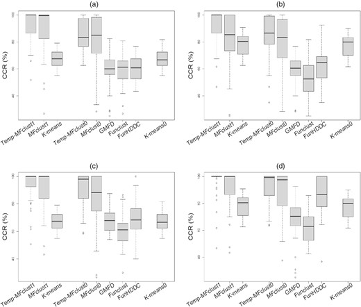
Clustering results of the simulation study in Section 3.2: correct classification rates (CCR) by different methods for each of the four cases of between-cluster separation; (a) fWeak-coWeak; (b) fWeak-coStrong; (c) fStrong-coWeak; (d) fStrong-coStrong. The sample size combination is .
Additionally, we investigated how much of dimension reduction occurs in applying the proposed MFclust1 by monitoring the estimated number of factors through the MCMC sampling. Figure S19 shows that the estimated number of factors (r) is much smaller than the original dimension () of the joint vector of basis coefficients and covariates. Finally, we conducted sensitivity analysis to check if the results are robust to different choices of hyperparameters for the DP and IBP in applying the proposed MFclust1 and MFclust0. Figure S20 indicates that clustering results are quite robust to varying choices of hyperparameters.
4 DATA APPLICATION
In this section, we apply the proposed models to the air pollution data described in Section 1. In Section 4.1, we cluster the annual trajectories of the daily mean concentrations of , and in 2010, while incorporating the spatial coordinates and two socio-economic indicators. In Section 4.2, we conduct clustering of the annual trajectories of and in 1987, 1992, 1997, 2002, 2007 and 2012 with temporal dependency while incorporating the spatial coordinates.
4.1 Clustering the annual trajectories of , and in 2010
We analysed the time-series data for daily mean concentrations of , and collected from 25 cities in Canada in 2010. We consider the spatial coordinate (i.e., latitude and longitude), GDP and %Unemp as city-specific covariates. We apply the proposed model described in Section 2.1, both with and without city-specific covariates, abbreviated as 'MFclust1' and 'MFclust0', respectively. Before clustering, we standardise each covariate. We use the reparametrized cubic B-spline basis with 20 equidistant internal knots. For posterior sampling, we truncate the DP with , for which the truncation error bound is calculated as with and . We set the hyperparameters as follows: and . We run the MCMC algorithm for 15,000 iterations and discard the first 10,000 samples as burn-ins.
Figure 5a–d shows the clustering results from MFclust0. Without incorporating the covariates, two clusters were identified (Table S1 lists the names of cities in each cluster). Cluster 1 (black) includes 23 cities (92 ), for which the annual trajectory of peaks in April and troughs in October with large amplitude (Figure 5a), while the level of peaks in February and troughs in August with small amplitude (Figure 5b). The level of shows wiggly trajectories with small amplitudes. Cluster 2 (red) includes two cities (8 ), Calgary and Edmonton, for which the level of peaks in April and troughs in January, whereas the level of shows an opposite trajectory with a peak in January and a trough in July. The level of shows wiggly trajectories. All three trajectories in cluster 2 show larger amplitudes than those of cluster 1.
![Clustering results of the data application in Section 4.1: (a)–(c) and (e)–(g) cluster-specific mean curves with 95 % credible intervals for O3, NO2 and PM2.5 estimated from MFclust0 and MFclust1; (d), (h) map of clusters obtained from MFclust0 and MFclust1; (i) scatter plot for gross domestic product and unemployment rate with clusters indicated [Colour figure can be viewed at https://dbpia.nl.go.kr]](https://oup.silverchair-cdn.com/oup/backfile/Content_public/Journal/jrsssc/71/5/10.1111_rssc.12589/1/m_rssc12589-fig-5.jpeg?Expires=1749138626&Signature=GtySlvhriqjGAe7hyAh86am-J327ZWD2sErr3NKH3VYlf7QoNOOhpie~C1vFVjEMWYIIuxE9hf6WgZMRzDfsBnRJ4PRm4jEOESfOPB7a-kMXxPMv8IKz9zSTWqUmZZLm~lCvp-EBMXDO4SWX3vSmm6ImynySL9CK96jZZ9yOjg-G45y9PmLCUz7IWBbaPcoiN8DTCgVRB21H3GHus08jQTyZoWOPLC9tnS~vgRmtzI0CAJR0wlMJZGGrm1DbT~LykBPAyN6Vqa6fWR0-o0kqqWgVtFWrYvNnNVt6E1SVdR-ZFZyKGU412~Nn1sxeFbL2Ocexb2rjC3jeatvMJVlfWA__&Key-Pair-Id=APKAIE5G5CRDK6RD3PGA)
Clustering results of the data application in Section 4.1: (a)–(c) and (e)–(g) cluster-specific mean curves with 95 credible intervals for , and estimated from MFclust0 and MFclust1; (d), (h) map of clusters obtained from MFclust0 and MFclust1; (i) scatter plot for gross domestic product and unemployment rate with clusters indicated [Colour figure can be viewed at https://dbpia.nl.go.kr]
Figure 5e–i shows the clustering results from MFclust1. By incorporating the spatial coordinate, GDP and %Unemp, three clusters were identified (Table S2 lists the names of cities in each cluster). Compared with MFclust0, MFclust1 clustered the cities that are geographically more adjacent and similar in socio-economic conditions while clustering based on the annual trajectories of , and . Cluster 1 (black) includes 17 cities (68 ) that are located in the east which show low GDP and relatively high levels of %Unemp (Figure 5h,i). Cluster 2 (red) is equivalent to cluster 2 identified by MFclust0, which includes the two cities, Calgary and Edmonton. Incorporating the GDP and %Unemp into clustering revealed that these two cities have much higher level of GDP and lower level of %Unemp. Finally, cluster 3 (blue) includes western six cities that show low GDP and low %Unemp and the seasonal fluctuations in the levels of and are similar to cluster 1.
Overall, our results indicate that the cities with higher GDP (Calgary and Edmonton) showed larger amplitude in the seasonal patterns of , and , and higher levels of throughout the year. In addition, western cities showed lower level of than eastern cities based on the results of clustering with the spatial coordinates.
4.2 Clustering the annual trajectories of and in 1987–2012 with temporal dependency
We analyse the time-series data for daily mean concentrations of and collected for 25 cities in 1987, 1992, 1997, 2002, 2007 and 2012. For city-specific covariates, we include spatial coordinates. We apply the proposed model described in Section 2.2, with and without city-specific coordinates, denoted by 'Temp-MFclust1' and 'Temp-MFclust0', respectively. For the basis, we use a reparametrised cubic B-spline basis with 20 equidistant internal knots. For posterior sampling, we truncated the dHDP with in the stick-breaking representation of . The hyperparameter is set as follows: . We run the MCMC algorithm for 25,000 iterations and discard the first 20,000 samples as burn-ins.
Since the results from the Temp-MFclust1 and Temp-MFclust0 are similar, we present only the result of the Temp-MFclust1 in Figure 6 (see Figure S22 and Table S3 for the result of Temp-MFclust0). By incorporating the spatial coordinate, five clusters were identified (Table S4 lists the names of cities in each cluster in the years 1987, 1992, 1997, 2002, 2007 and 2012). Figure 6a,b shows the cluster-specific mean curves for and . Figure 6c–h shows how the spatial pattern of the clusters changed over time. In 1987 (Figure 6c), the cities around Toronto belonged to cluster 2 (red) while most of the other cities belonged to cluster 1 (black). However, in 2002 (Figure 6f), none of the cities remained in clusters 1 and 2 as the cities around Toronto moved to cluster 5 (cyan) and other cities moved to cluster 3 (blue) and 4 (green), which remain roughly the same in 2007 and 2012.
![Clustering results from the Temp-MFclust1 in data application of Section 4.2; (a) and (b) cluster-specific mean curves with credible intervals for O3 and NO2, respectively; (c)–(h) map of clusters in 1987, 1992, 1997, 2002, 2007 and 2012, respectively [Colour figure can be viewed at https://dbpia.nl.go.kr]](https://oup.silverchair-cdn.com/oup/backfile/Content_public/Journal/jrsssc/71/5/10.1111_rssc.12589/1/m_rssc12589-fig-6.jpeg?Expires=1749138626&Signature=mbbQpH8yF7JQ6qajFfrCIIb4Ij8KjfhhN2GqU8MUXTrYIUfKmri8rjGh884lLZQPOETrX06ZhEINQoZ98FYAMx36EbsgFkJtbNrGsri3nrk5pGciPHXLJ5XcEI~L~4RShgINrNKKtXeD85fUtKlJhae3JALSvTeGOs3UxkgwaLWGkYfYvmU7Qit2u9aTlFdsD8ChEYDODFg9pMmlfSKornITfQZ~i-L4zbKhWYfpel2W7rND9kDY3iorc3hjjbvuc1xx6f-gFbX8Oeyge36rIReHM4OYgkcZPPJM5MF~6~cEhB4Laltr4Y8zuCbAzEQKxzZk2pdQ51wpu40UJkOurw__&Key-Pair-Id=APKAIE5G5CRDK6RD3PGA)
Clustering results from the Temp-MFclust1 in data application of Section 4.2; (a) and (b) cluster-specific mean curves with credible intervals for and , respectively; (c)–(h) map of clusters in 1987, 1992, 1997, 2002, 2007 and 2012, respectively [Colour figure can be viewed at https://dbpia.nl.go.kr]
These results imply that, in earlier years, most of the cities showed lower levels of and higher levels of , similar to the trajectories of clusters 1 and 2. However, the cities around Toronto have changed the seasonal patterns, showing higher levels of and lower levels of . In addition, the two cities, Calgary and Edmonton, changed the seasonal curve of dramatically from 1997, showing a U-shaped seasonality with a higher level of in winter. Overall, our results indicate that the annual trajectories of and have changed, showing temporal dependency from 1987 through 2012 in Canada in most of the 25 cities.
5 DISCUSSION AND CONCLUSION
In this paper, we propose a non-parametric Bayesian sparse latent factor model for covariate-dependent multivariate functional clustering and apply it to cluster the seasonal curves of multiple air pollutants incorporating location-specific covariates. We further extend the model to cluster the seasonal curves observed in multiple years with temporal dependency. Simulation studies show that our proposed models perform better than other competing methods. Our data application reveals that the annual trajectories of the levels of , and for 25 cities in Canada are grouped into two or five clusters, the geographical and socio-economic indicators seem to play a role in clustering the seasonal curves of pollutants, and the clustering structure has changed over the decades with temporal dependency.
In functional data clustering, basis expansion representation of functional data is a frequent solution for dimension reduction. One of the widely used tools to represent the functional curves through a low-dimensional vector is a FPCA (Jacques & Preda, 2013, 2014; Schmutz et al., 2020), where a finite number of basis functions are derived by eigen decomposition of the empirical covariance function of the observed curves, and each curve is then represented by a vector of eigenscores with respect to the estimated basis. It has been proven that an equivalent representation of the functional curve to the FPCA approach can be obtained if an orthonormal basis (i.e., Fourier basis) is chosen and a usual multivariate PCA is applied to the corresponding basis coefficients (Ramsay & Silverman 2005). Our proposed methods rely on the basis expansion with a cubic B-spline basis with reparametrisation, which does not lead to an equivalent formulation to the FPCA approach. This may be regarded as a drawback of the proposed model from the FPCA point of view. However, by including a sparse latent factor model within the hierarchy, our model leads to an analogous formulation to the FPCA approach as noted in Montagna et al. (2012). Additionally, orthogonality in the basis enhances interpretability of the elements in the eigen-decomposition, but this is not a primary concern in our application since our aim is to conduct a covariate-dependent functional clustering and a sparse latent factor model with basis function approach is adopted as a dimension reduction tool while linking the functional data with a covariate vector which is potentially high-dimensional.
In sparse Bayesian latent factor modelling, there are other alternative priors than the IBP for the factor loading matrix such as the multiplicative gamma process shrinkage prior (MGP) (Bhattacharya & Dunson, 2011). While the IBP induces sparsity by generating a binary matrix which allows for many of the factor loadings to be zero, the MGP makes the elements in the loading matrix to shrink towards zero as the column index increases. Thus, a loading matrix generated from the MGP has infinitely many nonzero columns, and one needs to truncate the number of columns with an adaptive procedure in the MCMC sampling for practical use. Furthermore, Durante (2017) noted that in using the MGP, the desirable shrinkage property is not guaranteed if the hyperparameters are not carefully chosen depending on the model. Recently, Legramanti et al. (2020) proposed an alternative prior, called a cumulative shrinkage prior (CSP), to overcome such limitation of the MGP. Though the CSP was shown to perform better than the MGP in their simulation study, it was not compared with the IBP. Future research on the comparison of these priors would be warranted to provide guidelines to practical users.
As our proposed models rely on the MCMC sampling to approximate the posterior distributions for inference, it takes much longer time to fit the proposed models than to fit the competing models. For example, in Section 3.1, it took 5 min 45 s for the 15,000 MCMC iterations to fit the MFclust1 for the sample size combination of . Meanwhile, it took 0.66, 12.01, 0.58, 15.08, and 0.51 s for the competing methods of K-means, GMFD, Funclust, FunHDDC and K-means0, respectively. In Section 3.2, it took 11 min 40 s for the 25,000 iterations to fit the Temp-MFclust1 while 1,49, 1.06, 1.75, 1.81, and 0.51 s were taken for each of the competing methods. These quantities rely on an R (R Core Team, 2020) implementation run on an Intel Core i9-9900KF CPU desktop computer with 64GB of RAM. The increased computing time may be a drawback of our proposed methods, but it should be worth spending to obtain better clustering results.
The proposed models are motivated by a problem of clustering the seasonal curves of multiple air pollutants, but they can be applied to a general setting of multivariate functional clustering when incorporating covariates or/and temporal dependency is desired. Our models do not require the functional data to be completely observed or observed at equally spaced grid points. Because we obtain a lower-dimensional representation of the functional data through basis expansion, our methods can be applied to multivariate functional data that are observed sparsely or at unequally spaced grid points. In addition, our model can accommodate either continuous or categorical covariates, which should be useful in many applications such as social science, biology, and epidemiology.
DATA AVAILABILITY STATEMENT
The data that support the findings of this study are available on request from the corresponding author. The data are not publicly available due to privacy or ethical restrictions.R and C++ code used in this article is available at the Github website (https://github.com/yangdw01/MFclust) and the data used in the application can be requested from the corresponding author ([email protected]).
ACKNOWLEDGEMENTS
This research was supported by the Senior Research grant (2019R1A2C1086194) from the National Research Foundation (NRF) of Korea funded by the Ministry of Science, Information and Communication Technologies, the Basic Science Research grant (2019R1A2C1010018) from the NRF of Korea funded by the Ministry of Education, and the Government-wide R D Fund project for Infectious Disease (HG18C0025).
REFERENCES
Author notes
Funding information Government-wide R & D Fund project for Infectious Disease Research, HG18C0025; National Research Foundation of Korea, 2019R1A2C1086194; 2019R1A2C1010018
