


Abstract
Studies of species distribution patterns traditionally have been conducted at a single scale, often overlooking species–environment relationships operating at finer or coarser scales. Testing diversity-related hypotheses at multiple scales requires a robust sampling design that is nested across scales. Our chief motivation in this study was to quantify the contributions of different predictors of herbaceous species richness at a range of local scales.
Here, we develop a hierarchically nested sampling design that is balanced across scales, in order to study the role of several environmental factors in determining herbaceous species distribution at various scales simultaneously. We focus on the impact of woody vegetation, a relatively unexplored factor, as well as that of soil and topography. Light detection and ranging (LiDAR) imaging enabled precise characterization of the 3D structure of the woody vegetation, while acoustic spectrophotometry allowed a particularly high-resolution mapping of soil CaCO3 and organic matter contents.
We found that woody vegetation was the dominant explanatory variable at all three scales (10, 100 and 1000 m2), accounting for more than 60% of the total explained variance. In addition, we found that the species richness–environment relationship was scale dependent. Many studies that explicitly address the issue of scale do so by comparing local and regional scales. Our results show that efforts to conserve plant communities should take into account scale dependence when analyzing species richness–environment relationships, even at much finer resolutions than local vs. regional. In addition, conserving heterogeneity in woody vegetation structure at multiple scales is a key to conserving diverse herbaceous communities.
INTRODUCTION
Ecologists have been trying for many years to arrive at a comprehensive description of species distribution patterns and the mechanisms explaining these patterns (Gaston 2000; Rosenzweig 1995; Whittaker et al. 2001). Studies of species distribution patterns and of correlations between species and environment traditionally have been conducted at a single scale of observation. There is an increasing recognition that different types of ecological processes that influence species richness are important drivers at different scales (Allen et al. 1984). For example, Crawley and Harral (2001) suggested that at small scales (1 m2 or less), ecological interactions are the most important processes controlling plant diversity in a system, but at larger scales, drivers such as topography, management, geology and hydrology are more important because they influence habitat type. Although variability and spatial configuration of ecological processes and environmental factors should have effects on species distribution at all scales, their effects may vary, as the relative importance of the underlying ecological drivers may change across scales. Thus, studies conducted at a single spatial scale may overlook species–environment relationship patterns at finer or coarser scales (Best and Stauffer 1986). Therefore, in order to maintain biodiversity, it is crucial to examine species–environment relationships at multiple spatial scales (Perevolotsky 2005).
A number of approaches have been used to develop predictive models for species–environment relationships. Common to most of these approaches is the use of topography, soil and climate as predictors (Davies et al. 2005; Stohlgren et al. 2000, 2005) and only seldom has woody vegetation been incorporated as an important determinant of species distribution (Jones et al. 1994; Shachak et al. 2008). Organisms can affect their immediate environment, and they do so in proportion to the scale and nature of their activity. In terms of their impact on species composition and richness, woody plants can be considered dominant factors that have an extensive effect on their environment, changing resource distribution in space and time (House et al. 2003). Small-scale environmental modifications caused by trees and shrubs have been widely investigated in arid and semiarid systems (Haworth and McPherson 1995; Holzapfel et al. 2006; Tielbörger and Kadmon 1997). The effects of woody vegetation on herbaceous species can occur via amelioration of harsh environmental conditions, alteration of substrate characteristics or increased resource availability (Belsky and Canham 1994; Callaway 1995). Experimental manipulations suggest that factors related to soil fertility (Belsky and Canham 1994) and amelioration of radiant-energy regimes (Parker and Muller 1982) show a range of interactions that influence herbaceous production. Woody vegetation may affect herbaceous vegetation via rainfall interception (Maestre, Cortina et al. 2003), litter accumulation (Moro et al. 1997), shading (Maestre et al. 2003), alteration of soil moisture (Maestre et al. 2003) and enhancement of soil nutrient pools (C, N, P and cations; Cortina and Maestre 2005), or a combination of these factors. These effects depend on leaf area, canopy architecture and rooting patterns of the woody vegetation (Padien and Lajtha 1992; Schlesinger et al. 1996; Scholes and Archer 1997). Mediterranean ecosystems, commonly referred to as vegetation mosaics, are highly heterogeneous at a broad range of spatial scales, starting from a grain size as small as a few meters (Bar Massada et al. 2008; Di Castri et al. 1981; Naveh 1975; Noy-Meir et al. 1989; Pausas 1999; Shoshany 2000). The fine-grained mosaic is characterized by woody patches at different heights and sizes, herbaceous clearings, exposed rocks and bare ground (Perevolotsky et al. 2002). Thus, we expected that the major effect of woody vegetation on plant species would be manifested chiefly at fine scales.
Many studies that explicitly address the issue of scale do so by comparing local (up to tens of square meters) and regional scales (spanning broad geographic ranges; Belote et al. 2009; Bosch et al. 2004). Our chief motivation in this study was to quantify the contribution of several predictors of herbaceous species richness at a range of local scales. We address two hypotheses, which pertain to Mediterranean landscapes as well as to a more general ecological context: (i) the relative importance of various environmental predictors of herbaceous species richness will be scale dependent even for a narrow range of scales (10–1000 m2); and (ii) the impact of woody vegetation on the richness of herbaceous species will be expressed chiefly at fine scales (10 m2), whereas the impact of topography and soil will be expressed chiefly at coarse scales (1000 m2).
MATERIALS AND METHODS
Study site
The study was conducted in Ramat Hanadiv Nature Park, located at the southern tip of Mt Carmel in northern Israel (32°309N, 34°579E), an area of 4.5 km2 surrounded by human settlements and agricultural fields. The area is a plateau located at an elevation of 120 m a.s.l. The soil is mainly Xerochrept, developed on hard limestone or dolomite (Kaplan 1989). The climate is eastern Mediterranean, characterized by relatively cool, wet winters and hot, dry summers. The vegetation is mostly eastern Mediterranean scrubland, dominated by dwarf shrubs (Sarcopoterium spinosum), low summer deciduous shrubs (Calicotome villosa), evergreen medium shrubs (Pistacia lentiscus) and tall evergreen shrubs (Phillyrea latifolia). Additionally, there are several scattered planted forest groves in the area, consisting mostly of conifer plantations (mainly Pinus halepensis, Pinus brutia and Cupressus sempervirens). The area has very rich herbaceous flora (Hadar et al. 1999).
Field sampling
In the spring of 2007, we recorded vascular plants using 4374 quadrats of 20×20cm. Plant species were identified by a team of botanists. A total of 325 herbaceous species were recorded. Table 1 presents the mean number of herbaceous species sampled in each scale.
minimum, maximum and mean of the number of herbaceous species found in each scale
| Scale (m2) | Minimum | Maximum | Mean |
|---|---|---|---|
| 10 | 0 | 55 | 15.89 |
| 100 | 0 | 64 | 30.73 |
| 1000 | 15 | 100 | 55.74 |
| Scale (m2) | Minimum | Maximum | Mean |
|---|---|---|---|
| 10 | 0 | 55 | 15.89 |
| 100 | 0 | 64 | 30.73 |
| 1000 | 15 | 100 | 55.74 |
Testing hypotheses regarding diversity at multiple scales requires a robust sampling design that is nested and balanced across a wide range of scales. Such a design has rarely been applied before in ecological studies (Noda 2004; Urban 2002). We developed a hierarchically nested sampling design that is balanced across scales (Fig. 1). This means that when ascending from smaller to larger units, the change in scale is consistently incremental. Each sampling unit comprised three subunits of the next lower level. For example, three sampling units of 20×20cm were nested within one sampling unit of 1 m2 and three sampling units of 1 m2 were nested within one sampling unit of 10 m2. Overall, this sampling scheme was nested within two units of 1 km2 each (Fig. 1). The exact geographic coordinates of each 10 m2 quadrat were verified using real-time kinematic global positioning system with a precision of 1–2cm. Species richness at each of the examined scales—10, 100 or 1000 m2—was calculated as the total number of species observed in all quadrats located in each unit (Fig. 1).
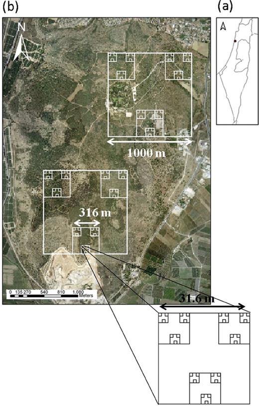
(a) location of the study site in Israel. Circle indicates Ramat Hanadiv Nature Park. (b) Aerial photo of Ramat Hanadiv study site and the hierarchical sampling scheme used in this study. The figure shows the scale ranging from 106 through 1 m2.
Environmental variables
We tested three sets of environmental variables: soil, woody vegetation pattern and topography, selecting two variables for each set. We tested all of the variables for multicollinearity by examining cross-correlations among variables; in all cases, cross-correlations were lower than 0.6.
Soil
A single soil sample was collected in each 10-m2 sampling unit using the sampling design described in the previous section (Fig. 1). The surface litter, if present, was removed, and the top 5cm of soil was sampled. Samples were air-dried and passed through a 2-mm sieve, then ground in a three-ball grinder.
In order to characterize soil properties, we selected three major soil chemical traits, which together provided a general understanding of the soil: pH, CaCO3 and organic matter. We used photoacoustic spectroscopy, which is a spectral technique that is rapid and inexpensive relative to the conventional methods of soil characterization (Du et al. 2007; Linker et al. 2005). Fourier-transformed infrared photoacoustic spectroscopy is based on the absorption of electromagnetic radiation by the sample and nonradiative relaxation that leads to local warming of the sample. Pressure fluctuations are then generated by thermal expansion, which can be detected by a very sensitive microphone. This method allowed us to characterize large areas at high resolution.
For 417 samples, we determined the pH, CaCO3 and organic matter concentrations using photoacoustic spectroscopy. Quantitative analysis of the spectra was performed using partial least squares. The samples were split randomly into calibration and validation sets, containing 75% and 25% (whose pH, CaCO3 and organic matter concentrations were determined by conventional chemical methods) of the samples, respectively. The root mean square of the determination errors was used to estimate model performance (for a detailed description of the method, see Du et al. 2008). Plotting the predicted versus the actual values of the validation data revealed that CaCO3 and organic matter had high R2 values (0.97 and 0.72, respectively), whereas pH had low R2 value (0.3). Consequently, pH was excluded from further analysis.
Each soil sample represented one sampling unit of 10 m2, and respective averages were calculated for 100- and 1000-m2 units.
Woody vegetation patterns
Woody vegetation pattern was characterized by the percentage of woody cover and woody vegetation height. A binary map of woody and nonwoody vegetation was generated from a digital color orthophoto of the study area (Fig. 1). Woody cover was quantified for each sampling unit using FRAGSTATS software (McGarigal et al. 2002).
Vegetation height was assessed by Ofek™ aerial photography acquired in 2005 with an Optech™ ALTM2050 LiDAR (light detection and ranging) system, using the single-return method with a horizontal spacing of ~2 m between points. The vertical accuracy of the LiDAR points was 0.15 m, and the planimetric accuracy was 0.75 m.
Topography
Initially, topography consisted of four variables: elevation, slope, north–south and east–west components of aspect. The east–west gradient had the lowest explained variance at all scales and was therefore excluded from the analysis. Elevation was also excluded from the analysis, as it had significantly high correlation with the other two variables.
Aspect and slope were determined for each sampling plot using a digital elevation model (pixel size = 2 m). The north–south component of aspect is a variable ranging from 0–180°, where north = 0°, south = 180° and east = west. Slope and aspect were averaged to derive values for the 10, 100 and 1000 m2 plots, respectively.
Spatial variables
The presence of spatial autocorrelation within ecological data results in a lack of independence of data points (Legendre and Legendre 1998; Lichstein et al. 2002). In order to quantify and remove the spatial autocorrelation effects from the analysis, we included spatial variables constructed from the geographic coordinates (X, Y) of each plot (Borcard et al. 1992; Hobson et al. 2000; Legendre 1993). We generated a cubic trend surface polynomial with nine variable terms (the geographic coordinates (X, Y), as well as X2, Y2, XY, X3, Y3, X2Y and XY2), which is appropriate for capturing broad-scale spatial trends (Lichstein et al. 2002).
Data analysis
We used redundancy analysis (RDA; ter Braak and Prentice 1986) to quantify the variance explained by the environmental and the spatial variables. In RDA, a univariate response variable is predicted by a standard linear multiple regression, and the variance is quantified by sum-of-squares (Birks 1996; Okland et al. 2006; ter Braak and Smilauer 2002).
In the RDA for species richness, spatial variables were considered covariables in order to remove their effects. For each analysis, we recorded the statistical significance, as measured by a Monte Carlo unrestricted permutation test with 499 permutations of all canonical axes (ter Braak and Smilauer 2002).
The significance of each explanatory variable was measured using a Monte Carlo permutation test with 499 randomizations. These analyses were conducted with CANOCO version 4.5 (ter Braak and Smilauer 2002). For each analysis, we recorded the sum of canonical eigenvalues and divided it by the total variation in the species data (total inertia) to estimate the proportion of the total variance explained by a set of variables (Greenacre 1984). To calculate the proportion of the total variance explained by each specific variable (also termed marginal contribution), we divided the explained variance singly (i.e. using this particular variable as the only environmental variable) by the total inertia.
We used variation partitioning approach to determine both the pure and the shared effects of the six environmental predictors on plant species richness at each scale (Cushman and McGarigal 2002), using a series of (partial) regression analyses with RDA (for full description of the method, see Cushman and McGarigal 2002).
Geostatistic analysis
Geostatistic analysis was applied to quantify the range of variability of each predictor. Semivariance analysis examines the contribution of all pairs of points that are separated by a given distance (lag) to the total sample variance. We fitted an exponential model to the distribution of the semivariances as a function of their lag distances, using GS+ (Gamma Design Software).
The nugget-to-sill ratio was used to classify the spatial dependence of the environmental variables (Table 2; Cambardella et al. 1994). If this ratio was smaller than 0.25, then the variable was considered to be spatially dependent or strongly distributed. When this ratio was between 0.25 and 0.75, the variable was considered to be moderately spatially dependent.
variogram model parameters for all environmental variables
| Variable | Nugget (C0) | Sill (C0 + C) | Range (m) | C0/C0 + C |
|---|---|---|---|---|
| Woody cover % | 95 | 929 | 24 | 0.102 |
| Vegetation height (m2) | 0.001 | 1.999 | 36 | 0.001 |
| Northness Angle | 50 | 7 210 | 2 502 | 0.007 |
| Slope Angle | 5.38 | 16.69 | 204 | 0.322 |
| CaCO3 (g[CaCO3]/g[dry soil]) | 7.4 | 105 | 105 | 0.070 |
| Organic matter (mg[OM]/g[dry soil]) | 100 | 945 | 21 | 0.106 |
The model fitted to the semivariogram quantified the scale of heterogeneity (patch size, Ettema and Wardle 2002), meaning the scale at which the variability is the largest. For example, in fine-scale heterogeneity, there are many small and fragmented patches (Fig. 2a) and in coarse-scale heterogeneity, there are only a few large patches that are continuous (Fig. 2b).

an insulation of fitted models to the semivariogram quantifies the scale of heterogeneity (patch size): (a) fine-scale heterogeneity; (b) coarse-scale heterogeneity.
RESULTS
Species richness
The percentage of the total variance explained by each group of variables varied across spatial scales (Fig. 3). Woody vegetation was the dominant group of predictors at all scales (over 90% of the explained variance for both fine and medium scales); however, its explanatory power was smaller at coarse scale (about 60% of the explained variance). Soil variables were a more important group of predictors at the coarse scale (39%) compared withat the fine scale (12%). Topography explained a greater percentage of variance at coarse scale (39%) than at fine scale (26%).
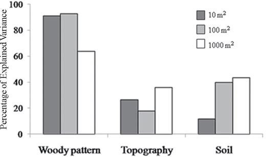
the variance explained by the three groups of predictors of species richness given as percentages of the total explained variance.
Among the different predictors comprising the three groups of variables, woody cover accounted for the highest percentage of the explained variance at all three scales (Fig. 4). The percentage of the explained variance of three variables varied considerably across scales: woody cover decreased by 42%, CaCO3 increased by 250% and organic matter increased by 316% between fine and coarse scales (Fig. 4). At all scales, species richness was (i) negatively related to vegetation cover and height, slope and CaCO3 and (ii) positively related to northness.
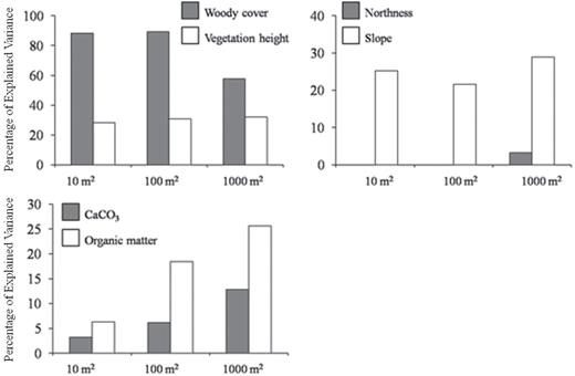
the variance explained by the six environmental predictors of species richness given as percentages of the total explained variance.
Decomposing the explained variation in species richness datasets into variation components showed clear differences between predictors and between scales. In general, the variation partitioning revealed that most of the explained variation in species richness at all three scales was related to woody pattern and that the explained variation was smaller at the coarse scale (Fig. 5). Soil and topography groups of variables explained more variation at the coarse scale than at the finer scales (Fig. 5). The largest pure effect at all three scales was of woody cover. The pure effect of two variables varied considerably across scales: woody cover decreased by ~10%, and organic matter increased by 8.5% between fine and coarse scales (Fig. 4). Overall, these results were congruent with the results of the previous analysis.
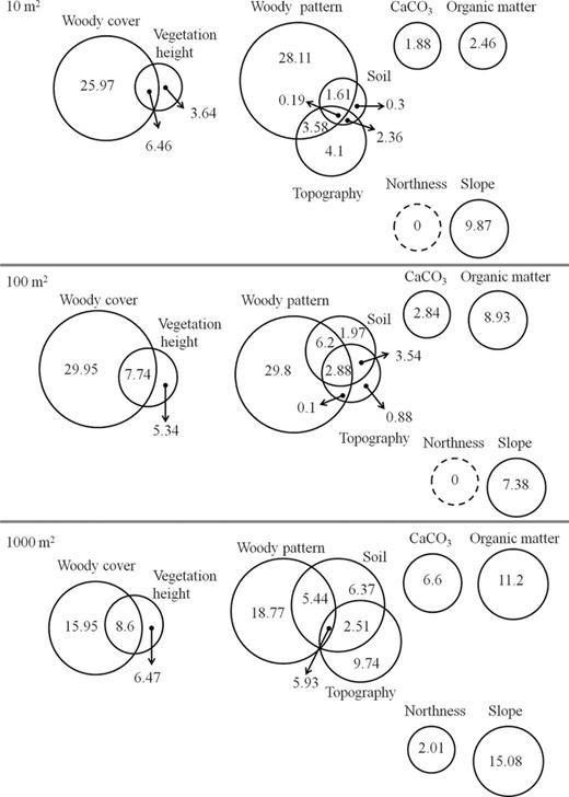
results of variation partitioning (%) of the six environmental predictors at the three studied scales. The areas of the circles represent the fraction of total variability explained.
Geostatistic analysis
We used semivariogram analysis to describe the scale of heterogeneity of the six environmental variables (Table 2). All of the empirical semivariograms fit well to the exponential model, indicating the existence of spatial dependence. The total variance explained by the structural variance (spatial dependence) was high and ranged between 0.678 and 0.999. The nugget-to-sill ratio showed a strong spatial dependence for all variables except slope, which showed moderate spatial dependence. The range of variability varied greatly between the environmental variables. Woody cover, vegetation height and organic matter had small ranges, indicating fine-scale heterogeneity, whereas northness, slope and CaCO3 had large ranges, indicating coarse-scale heterogeneity (Table 2).
DISCUSSION
Do environmental determinants of biodiversity differ between scales?
The relationships between species richness and environmental variables varied considerably across scales, such that with the increase in scale, the effects of woody vegetation decreased and the effects of soil and topography increased. One possible explanation of this phenomenon is that the scale of heterogeneity of the environmental variables is different, as was revealed by the semivariogram analysis. Woody vegetation cover, vegetation height and organic matter can be considered three characteristics of woody vegetation. The maximum variability of all three parameters was found to be at the small scale, indicating fine-scale heterogeneity, whereas maximum variability for northness, slope and CaCO3 was found at broader scales.
Slope and aspect strongly affect the amount of solar radiation reaching the surface. Solar radiation influences soil moisture, soil temperature and water evaporation (Bennie et al. 2008). CaCO3 affects soil pH and thus controls nutrient availability for plants and mobility of these elements in soil (Sarmadian et al. 2010). CaCO3 content differs between soil types. For example, Rendzina has high CaCO3 content, whereas Hamra and Terra Rosa have low CaCO3 content (Du et al. 2007, 2008). Thus, CaCO3 is expected to be heterogeneous, particularly at large scales.
We should, however, be very careful when interpreting this particular result. When analyzing spatial data, one should keep in mind that the observed impact of a given predictor is affected by the spatial resolution at which it was measured. Therefore, a direct comparison between the impacts of different independent variables, measured at different spatial resolutions, may be misleading. This is an inherent problem in many spatially explicit studies, which is seldom addressed. However, this was not a problem when comparing the change in explained variance of the six variables across scales as we compared them at specific and well-defined scales.
Many studies that explicitly address the issue of scale do so by comparing local (up to tens of square meters) and regional scales (spanning broad geographic scale; Bosch et al. 2004; Boyero 2003; Grand and Cushman 2003). We showed that scale dependence between environmental variables and species richness is apparent at fine scales even for a narrow range of scales (10–1000 m2). We speculate that the scale-dependence pattern we observed would be even more obvious if a broader range of scales were examined. Our study shows that scale needs to be studied at much finer resolutions than local vs. regional.
The impact of woody vegetation on herbaceous species
Woody vegetation pattern was characterized by the percentage of woody cover and woody vegetation height. Using these variables, we were able to characterize the 3D structure of woody vegetation, as opposed to the 2D vegetation description in most studies of landscape effects on species distribution (Kie et al. 2002; Kumar et al. 2006). Researchers have suggested that vertical vegetation stratification affects plant species diversity (Kumar et al. 2006). For example, the spatial structure of the canopy in a forest greatly influences understory plant regeneration and succession patterns (Blank and Carmel 2012; Clark et al. 1996; Moeur 1997) and may affect community structure and biodiversity patterns. Sunlight penetration through the canopy is directly related to the 3D spatial pattern of vegetation and influences the interactions between organisms and their physical environments (Blank and Carmel 2012; Stohlgren et al. 2000).
In this work, we showed that woody vegetation affected plant species richness at all the studied scales, but its explanatory power at the coarse scale was smaller than that at the fine scale. As suggested by the variogram, the maximum variability of woody vegetation was found to be at fine scales. Mediterranean ecosystems are highly heterogeneous at a broad range of spatial scales, starting from a grain size as small as a few meters (Bar Massada et al. 2008; Di Castri et al. 1981; Naveh 1975; Noy-Meir et al. 1989; Pausas 1999; Shoshany 2000). Therefore, we expected that the major effect of woody vegetation on plant species would manifest chiefly at fine scales. However, we found that woody vegetation was the prominent group of variables at all three scales, accounting for between 60% and 90% of the total explained variance.
Separate studies found that in Mediterranean ecosystems, woody vegetation affects plant species richness at fine scales (up to tens of square meters, e.g. Agrawal 2001; Casado et al. 2004) and at broader scales (thousands of square meters; Atauri and de Lucio 2001); however, its effect across a narrow range of small scales has not been studied systematically.
The effects of woody vegetation on herbaceous species can occur via amelioration of harsh environmental conditions, alteration of substrate characteristics or increased resource availability (Belsky and Canham 1994; Callaway 1995). In addition, the effects of woody vegetation on its immediate environment were associated with the nurse-plant syndrome, in which seedlings of many species frequently overcome a harsh environment by growing below the canopies of adult shrubs or trees, where more benign conditions prevail (Franco and Nobel 1989; Lloret et al. 2005). Complex combinations of competition and facilitation operate simultaneously among plant species (Aguiar and Sala 1994; Callaway and Walker 1997; Chapin et al. 1994; Walker and Chapin 1986). Both negative interactions (interference; Grime 1979; Tilman 1988) and positive interactions (facilitation; Bertness and Hacker 1994; Callaway and Pugnaire 1999) change along gradients of resource availability, so that plant interactions are best viewed as dynamic relationships that depend on abiotic conditions. It has been suggested that positive interactions among plants are stronger in stressful areas, whereas negative interactions predominate in less stressful environments (Bertness and Callaway 1994). A study conducted along the aridity gradient in Israel found that the net effects of shrubs on annuals, expressed as relative interaction intensity, indicated a steady and consistent shift from net positive or neutral effects in the desert (most likely, the main causes are amelioration of drought stress by canopy shade or improved soil structure; Boeken and Orenstein 2001; Segoli et al. 2008) to net negative effects in the mesic part of the gradient (most likely, the main causes are competition for light, nutrients and water; Danin and Orshan 1990; Holzapfel et al. 2006; Shachak et al. 2008). Our study site is located in a Mediterranean ecosystem characterized by a less stressful environment than that of desert ecosystems. Thus, in accordance with Holzapfel et al. (2006), we found that the relationship between woody vegetation predictors and species richness was negative, implying negative net effect of woody vegetation on herbaceous plants. This result was consistent at all three scales.
Concluding remarks
Woody vegetation height and cover were found to be the most important environmental variables affecting species richness. The effect of woody vegetation on herbaceous species distribution has heretofore been relatively unexplored. In this study, it appears that woody vegetation is an important element in controlling the spatial distribution of herbaceous species across scales. This finding is important for conservation and management of biodiversity. Nowadays, it is possible not only to quantify the spatial pattern of woody vegetation in small and large areas using remote-sensing methodologies, but also to change its cover and spatial distribution using different management regimes, such as grazing, fire and clearcutting (Bar Massada et al. 2008; Henkin et al. 2007). In addition, this study shows that species–environment relationships are scale dependent. This means that generalization is very difficult and extrapolation should be undertaken with caution. In order to study species distribution, we recommend using a multiscale sampling scheme, enabling conclusions at different spatial scales concurrently.
FUNDING
The Eshkol Foundation of the Israel Ministry of Science and Technology.
This version was created to add an author name previously omitted.
ACKNOWLEDGEMENTS
We thank the botanists Yair Or, Bosmat Segal, Ran Lotan, Reut Luria, Rebeka Nukrian and Gabi Abraham. Special thanks to Liat Hadar and Ramat Hanadiv Nature Park officials for their help. We also thank Joshua Kob, Eyal Freedman, Noa Shmuelov, Sara Ellwood-Hofi, Michal Givoni, Roi Tamari, Adi Maymon, Amir Spiegel, Itay Halperin and Dvora Lotan for their help in the field work. Avi Perevolotsky has provided useful advice and productive comments. We thank Rafi Linker for his help with the soil characterization process.
REFERENCES


