Simulating the evolution of a clonal trait in plants with sexual and vegetative reproduction

Abstract

INTRODUCTION

Phenotypic optimality models of life-history evolution, such as evolutionary stable strategy (ESS) models, predict the evolution of an optimal phenotype (Metz et al. 1992; Waxman and Gavrilets 2005). For many phenotypic characters, the optimum occurs at intermediate trait values and optima at extreme trait values are an exception. However, in nature the evolution of a genotype corresponding to an optimal phenotype at intermediate trait values may be constrained by the genetic mechanisms of segregation, recombination and mutation. If intermediate phenotypes maximize fitness and allelic effects are additive, these phenotypes are expressed by heterozygous genotypes. In this case, evolution may not lead to the optimum predicted by an ESS because every recombination event will give rise to homozygotes corresponding to non-optimal phenotypes. Under idealized population dynamic assumptions of sexually reproducing organisms with non-overlapping generations, such fitness profiles characterized by selection for heterozygotes have been recognized to give rise to a stable genetic polymorphism (Hartl and Clark 1989).

However, many organisms have more complex life histories (Silvertown et al. 1997). Our study objects, clonal plants, have both sexual and vegetative reproduction, overlapping generations of ramets and genets and spatially explicit interactions between plant modules (Schmid 1990). Possibly due to the complexity of their life cycle, there are very few phenotypic and no gametic models (i.e. models explicitly including segregation and recombination and linking the allelic composition of genotypes to phenotypes) of the life-history evolution of clonal plants.

Among the few phenotypic models, some provide examples for intermediate phenotypic optima (Winkler and Fischer 2001). This led us to compare the outcomes of the evolution of clonal plant life histories in ESS models with gametic models in a situation where intermediate values of a phenotypic trait maximize fitness.

Sexual and vegetative reproduction differ in several phenotypic and genetic consequences (Sackville Hamilton et al. 1987). Phenotypic differences between the two modes of reproduction concern dispersal distance, timing of offspring production and establishment and the success of establishment. Moreover, both modes may be linked phenotypically by a trade-off in resource allocation (Prati and Schmid 2000). Genetically, vegetative offspring are identical to the parent, while genotypes of sexual offspring are determined by segregation and recombination. Lastly, a higher allocation to sexual reproduction may affect the rate of evolutionary change.

The fitness and population dynamics of clonal plants are affected by interactions of plant modules with spatially and temporally heterogeneous abiotic factors and with neighbouring plants and hence they depend on local density and on dispersal (Crawley and May 1987; Fahrig et al. 1994; Inghe 1989; Sintes et al. 2006; Winkler and Schmid 1995; Winkler et al. 1999). Dispersal of clonal offspring is often limited and may be further constrained by trade-offs, e.g. between the number of stolon branches and average stolon length (Meyer and Schmid 1999a; Sackville Hamilton et al. 1987).

The complexity of clonal life cycles and the need to consider spatially explicit interactions make the assessment of fitness very difficult for clonal plants as no analytical expression captures all determinants of clonal plant fitness. In earlier spatially explicit individual-based (SEIB) phenotypic models, we assessed clonal plant fitness as invasibility of a resident population by an immigrant phenotype (Metz et al. 1992) and showed that this fitness measure can approximately be predicted by single-phenotype simulations (Stöcklin and Winkler 2004; Winkler and Fischer 2001).

Fitness profiles obtained with these previous models revealed a number of situations where fitness was maximized at intermediate values of a phenotypic trait. For the gametic models presented here we used a spatially heterogeneous disturbance regime, where intermediate stolon internode length (distance between parent module and vegetative offspring) maximizes fitness because it optimizes the likelihood that vegetative offspring modules establish in empty sites after disturbance (Winkler and Fischer 1999, 2001).

Gametic models of life-history evolution explicitly couple phenotypes and underlying genotypes. In our study, we developed two types of gametic models. The first type considers the simplest case of one locus with two alleles and additive action of alleles; there were only three phenotypic values, i.e. three stolon internode lengths. Because most quantitative traits are affected by variation at few loci of large effect (Hall et al. 2006; Stearns and Hoekstra 2000), we also studied a second type considering the five-loci case with two alleles per locus of equal and additive effects, resulting in 11 different phenotypes.

We explored the evolution of stolon internode length with three model types that either were entirely phenotypic and spatially explicit (phenotypic SEIB model) or gametic, but not spatially explicit (‘Constant selection models’, see below) or both gametic and spatially explicit (gametic SEIB models). First, we calculated the fitness profile for the three, respectively 11, phenotypes with an entirely phenotypic spatially explicit SEIB model. Second, we used these fitness values in the widely accepted gametic, but not spatially explicit, constant selection model (CSM), where fitness values for different phenotypes are treated as fixed magnitudes independent of environmental variation (Hartl and Clark 1989). The CSM is in so far a gametic model as it considers the link between allele frequencies and fitness. Therefore, it allowed us predicting the frequencies of alleles, genotypes and phenotypes. However, while using constant fitness values obtained from single-phenotype SEIB simulations approximates the outcome of real evolution, it implies averaging over many stochastic demographic events and spatial interactions and it ignores density effects. Moreover, the CSM ignores genetic stochasticity. Furthermore, because only sexual reproduction is explicitly considered, the relative proportions of the sexual and vegetative modes of reproduction cannot be varied in such a model. Third, to overcome these shortcomings, we introduced segregation, recombination and mutation into more realistic gametic spatially explicit individual-based stochastic one-locus and five-loci simulation models (gametic SEIB models). Here, fitness of different phenotypes evolved during the interplay of demographic events and of intra- and interphenotype module interactions. Moreover, only the gametic SEIB models allowed us to study evolution for different proportions of vegetative and sexual reproduction.

We used the described models to derive (i) predictions from the fitness profiles in the one-locus and five-loci cases, (ii) fitness and allele frequencies evolving in the CSM, (iii) fitness and allele frequencies evolving in the gametic SEIB models under different degrees of sexual recruitment and with different mutation rates and (iv) the degree and role of locus fixation.

METHODS

Phenotypic model: the SEIB simulation model (phenotypic SEIB model)

We simulated plant population dynamics on a two-dimensional cellular grid consisting of 70 × 70 square cells arranged in a torus form (Winkler and Fischer 2001). Each of the cells could either be empty or host a part of a plant. We modelled growth, reproduction, dispersal and competition as stochastic events. The species we had in mind when developing the simulation models were perennials with vegetative and sexual reproduction.

We modelled module dynamics in annual steps. Each step included a sequence of four reproductive iterations each including module growth, seed production and seed dispersal, stolon formation, stolon elongation and establishment of vegetative offspring. Individual modules distributed over the grid were characterized by their property of reproducing either exclusively sexually with probability P_S or exclusively vegetatively with probability (1 − P_S) at the time of module birth (as in Watson et al. 1997). The probability of reproduction in each reproductive iteration depended on local density. According to its reproductive property, a module either produced N_S seeds or N_V stolons. Seed and stolon productions were modelled following Poisson distributions with parameters N_S0 and N_V0 and truncation at N_S = 1.2 N_S0 and N_V = 4, respectively. The standard values for vegetative and sexual fecundities were mean stolon number N_V0 = 2.0 and mean seed number N_S0 = 100. Parameters roughly correspond to field data for Prunella vulgaris (Winkler and Schmid 1995) or were chosen as in Winkler and Fischer (2001). After production, seeds were distributed randomly over the simulation grid and deposited in grid cells. Up to four stolons grew away from their parent modules with an internode length L_V, which was drawn from a uniform distribution between 0.9 L_V0 and 1.1 L_V0 (see (1) below). The branching angle α of the stolons was randomly varied by +10, 0 or −10 degrees from standard values. These standard values depended on the number of produced stolons and were 0 degree deviation from the parent stolon for one produced stolon, +60 and −60 degrees for two produced stolons, +60, 0 and −60 degrees for three produced stolons and two stolons with +60 and two with −60 degrees for four produced stolons (Winkler and Schmid 1995). The random variation ensured that all stolons had different branching angles. If a potential establishment site for an offspring module at the apex of a stolon was already occupied, establishment did not occur and the apex died. If several offspring modules competed for an empty microsite (grid cell), only one randomly selected one could establish. After establishment, modules were allowed to grow to a given full size and start reproduction. Maximal module size was three-by-three cells.

Once a year (in fall), disturbance gaps were created with a given probability and spatial extent. A disturbance event killed all affected modules together with their newly formed stolons, but did not affect seeds. After disturbance, seeds were allowed to germinate and seedlings established with probability P_E if the germination site was not occupied by other modules. Only one randomly selected seedling was allowed to establish per cell. Established seedlings grew and reached the reproductive potential in the next annual cycle.

The value for seedling establishment probability P_E determined the success of sexual reproduction relative to vegetative reproduction. For this study, we applied a disturbance scenario where each disturbance affected only cell (corresponding to the ‘small disturbances’ in Winkler and Fischer 2001) with a probability of disturbance of 0.3 for each cell.

Assessment of fitness

In the phenotypic SEIB model, we assessed long-term fitness of clonal plants as the relative competitive success of an invading phenotype against a resident stationary phenotype. Previously, we had derived an approximate expression for this measure of long-term fitness (competitiveness) from a simple additive model of vegetative and sexual reproduction (Winkler and Fischer 1999). It is a function of demographic parameters and parameters denoting the effectiveness of space utilization for reproduction. This fitness measure increases monotonically with stationary cover of a phenotype. We obtained the components of the fitness measure from the simulation model as given in Winkler and Fischer (2001). Here, we calculated it for each mono-phenotype population from simulations averaged over 50 years, where a stationary state had been reached in a forerun period of also 50 years.

With small disturbance gaps, phenotype fitness W (which had been called competitiveness in Winkler and Fischer 2001) depends unimodally on internode length L_V0 and hence on allele frequency f_a, i.e. fitness is maximized at an intermediate internode length (Winkler and Fischer 2001). This optimum is reached at parameter values c = 3.5, b = 2.0 in (1) below. At the optimal intermediate internode length that depends on the size and density of gaps, stolons preferentially meet disturbance gaps (Winkler and Fischer 1999). However, if internodes are shorter than the optimal length, offspring modules interact with their parent modules and fitness is decreased. Conversely, when internodes are longer than the optimal length, the likelihood decreases that offspring modules are placed in gaps, and fitness is also decreased.

Gametic models: combination of allele frequencies and phenotypes

To integrate genetics into the simulation model, we assumed two different gametic models:

• 1) One-locus model: one locus with two additively acting alleles a and A. This model gave rise to three different genotypes and phenotypes and three different values for the frequency f_a of allele a per genome, 0, 0.5 or 1.

• 2) One-loci model: five loci, each with two additively acting alleles a and A. The phenotypic effects of all alleles a and A were of the same magnitude and either negative (allele a) or positive (allele A). This gave rise to 243 different genotypes and 11 different ‘genotypic doses’ or frequency values f_a for allele a across the five loci.

In both gametic models, we assumed that the phenotype, i.e. the mean internode length L_V0, was linked to the frequency f_a of allele a in the genome of a module via

(1)

i.e. the higher the frequency f_a of allele a, the shorter the internode.

Moreover, because our previous study (Winkler and Fischer 2001) suggests an asymmetric fitness profile (also see Fig. 1 below), we also studied the importance of this asymmetry for the predictions of the one-locus gametic models by assuming different values of L_V0 for the aa homozygotes. These values ranged from 1.75 to 2.4, whereas the L_V0 values for AA homozygotes and heterozygotes were still given by (1).

Figure 1:

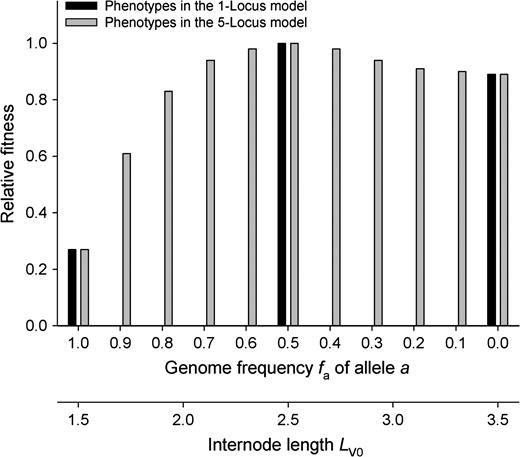
Relative fitness as a function of stolon internode length L_V0 and genotype allele frequency f_a with mean number of stolons N_V0 = 2 in the phenotypic SEIB model. Fitness was calculated for phenotypes with given stolon internode length. Values of f_a corresponding to the gametic models with one or five loci were linked with internode length L_V0 by (1).

Open in new tabDownload slide

Gametic CSM

The evolutionary processes of segregation and recombination, mutation and phenotypic selection lead to realized population allele frequencies p_aopt and p_Aopt = 1 − p_aopt. In the CSM (Hartl and Clark 1989), which is not spatially explicit and assumes constant fitness of a given genotype, p_aopt is determined by a maximization of population fitness W*. Here, W* as a function of p = p_a and q = (1 − p) = p_A is given by

(2)

where N = number of loci, r = genotype index and W_r+1 = fitness of phenotype linked to genotype r + 1. With given values for W_r+1, the optimum p_aopt of allele frequency a can be obtained by numerical evaluation. In the CSM, fitness values W_r+1 are assumed to be empirically obtained values known from previous field studies or experiments. In our context, they were obtained from single-phenotype SEIB simulations as described above.

Gametic SEIB models

Again, we defined the genotype of each module by the combination of alleles A or a at the one locus or five loci. Each flowering module acted as a seed-producing maternal module to which a paternal module was assigned at random from the set of all other flowering modules. To determine a new genotype separately for each seed, we simulated segregation and recombination by randomly sampling alleles from the paternal and maternal genomes for each locus, i.e. without any linkage disequilibrium. When we allowed for mutation, alleles were mutated with a small probability μ to the alternative one (A into a or a into A) at segregation (i.e. we did not consider somatic mutations here; see Orive (2001) for a model of the evolutionary fate of somatic mutations in clonal plants). To qualitatively demonstrate the effects of mutations, we used either unrealistically high μ = 0.01, to illustrate a very sharp contrast to the situation without mutations (μ = 0), or we used the still high, but more realistic value μ = 0.0001.

According to the frequency f_a of allele a in the module genome, a vegetative offspring module reached a certain parent–offspring distance L_V (stolon internode length) varying around mean L_V0 obeying (1). Thus, there was variation among genotypes in the distance between parent and vegetative offspring module and in the likelihood of the latter to meet disturbance gaps. Thus, the evolution of mean allele frequency p_aopt in the population was an inherent consequence of the spatially explicit simulation process.

We started evolutionary simulations with overall module densities similar to the stationary one. Initial allele frequency p_a of allele a in the module population was p_a0 = 0.5. The genotypic composition of the starting module population followed the Hardy–Weinberg distribution. We followed evolution in each simulation over a period of 600 and 3000 years. All results given here were averaged over 30 runs.

After 600 and 3000 years, respectively, we counted the number of fixed loci. In the one-locus case, we determined the proportion of runs that led to fixation, whereas in the five-loci scenario we averaged the proportion of fixed loci per run. It is important to note that complete fixation after 600 and 3000 years could also occur in the presence of mutations. Of course, at later stages mutations could reintroduce polymorphism into populations, which, however, was not the subject of the current study.

We parameterized sexual reproduction either to equal efficiency of resource utilization for both sexual and clonal reproduction, i.e. so that shifts in P_S, the percentage of sexual reproduction, did not lead to a shift in total population size (Winkler and Fischer 2001), or we assumed a lower efficiency of sexual reproduction, a situation common in clonal plants where vegetative offspring usually have higher rates of establishment than seedlings do (Meyer and Schmid 1999b). We achieved these two situations by setting the probability P_E of seedling establishment probability to either P_E = 0.0075 or P_E = 0.0025, respectively.

RESULTS

Fitness profiles

First we used the phenotypic SEIB simulation model to calculate fitness values (competitiveness) for different populations each consisting of only one phenotype. According to the two different gametic models, there were 3 and 11 different phenotypes representing all possible values of genome allele frequencies f_a and hence of stolon internode length L_V0. In both cases, L_V0 = 2.5 resulted in optimal fitness, corresponding to a frequency of allele a in the population of f_a = p_a = 0.5 (Fig. 1).

For a model of purely asexual evolution without any genetic changes, the distribution of fitness values of Fig. 1 implied that, starting evolution with a mixture of all possible genotypes, genotypes with f_a = 0.5 would outcompete all others. In the case of one locus, this would be the heterozygote. In the case of five loci, it could be one or more genotypes each with frequency f_a = 0.5.

Evolution in the CSM

Second, we used the CSM (2) to calculate mean population fitness W* corresponding to different preset values of population allele frequency p_a for the one-locus and five-loci gametic models (Fig. 2). Here, the fitness values W_r for the different possible genotypes were taken from Fig. 1.

Figure 2:

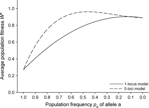
Average population fitness W* of modules of a clonal plant as a function of population allele frequency p_a(2) under consideration of genetic segregation, recombination and population dynamics according to the gametic CSM.

Open in new tabDownload slide

Under the assumptions of the CSM, fitness W* was optimized for population frequencies of p_aopt = 0.125 (one-locus model) and p_aopt = 0.45 (five-loci model). Thus, the predicted outcome of evolution in the one-locus model sharply differed from that of the purely phenotypic one (which corresponded to p_aopt = 0.5), whereas under the five-loci assumption the difference between the predictions of the gametic and phenotypic models was much smaller.

Evolution in the one-locus gametic SEIB simulation model

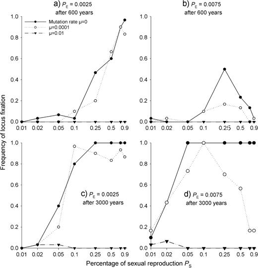
Third we simulated evolution of the model clonal plant with the one-locus gametic SEIB model. First, we modelled the case without mutations. If there was no sexual reproduction (proportion of sexual reproduction P_S = 0), the homozygous genotypes aa and AA were displaced by selection after 425 ± 120 years as expected from the phenotypic prediction due to the higher fitness of the heterozygous genotype (Fig. 1). As long as the proportion of sexual reproduction P_S became not too high, its increase pronouncedly decreased population allele frequency p_a from 0.5 (Fig. 3), reflecting that segregation and recombination became more important with higher sexual reproduction and thus allowed the population to evolve towards lower frequencies of the low-fitness short-stolon genotypes. Clearly, this was even more pronounced with higher seedling establishment probability P_E (cf. Fig. 3a and c with 3b and d, respectively). Allele frequency p_a even evolved to values <0.125, i.e. below the ones predicted by the CSM, illustrating that not only the maintenance of a variety of genotypes in the population due to recombination played a role but also the fixation of non-optimal genotypes.

Figure 3:

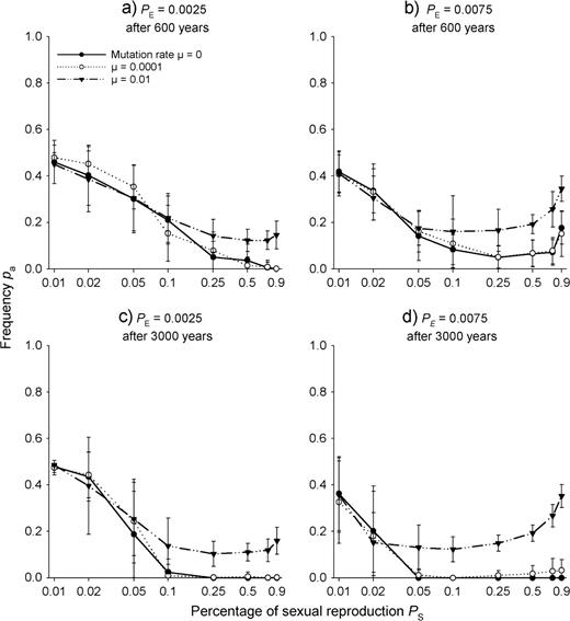
Population frequencies p_a of allele a in a stationary population of the clonal plant after evolution over 600 years (a and b) and over 3000 years (c and d) for different proportions of sexual reproduction P_S and different mutation rates μ. The gametic SEIB model assumed one locus with two alleles a and A linked to internode length L_V0 by (1). Shown are means and standard deviations from 30 runs. Simulations were done with two different values of seedling establishment probability P_E. The x-axis is log scaled.

Open in new tabDownload slide

However, especially at high values of seedling establishment P_E, with increasing proportion of sexual reproduction P_S, vegetative reproduction and therefore fitness-determining stolon internode length became less important. Therefore, after 600 years and beyond some critical value of the proportion of sexual reproduction P_S, population allele frequencies p_a evolved, which deviated less from 0.5 than the ones that had evolved at lower proportion of sexual reproduction P_S. However, after 3000 years, the unimportance of vegetative reproduction at higher sexual reproduction P_S and therefore lower selection pressure to maintain allele a in the population was reflected by fixation of allele A when only AA homozygotes with long internodes (i.e. the homozygotes with relatively high fitness) remained in the population (i.e. the population arrived at p_a = 0; Fig. 3c and d).

In our 70 × 70 cell system, low mutation rates (μ = 0.0001) prevented the evolutionary trap of complete displacement of heterozygotes aA and therefore allele a in the course of 600 and 3000 years at high proportions of sexual reproduction P_S and at high seedling establishment probability P_E, when sexual reproduction was frequent enough to reintroduce allele a via mutation (remember that we did not consider somatic mutations). With high mutation rates (μ = 0.01), allele a was never lost from the population, and changes of establishment probability P_E and increasing duration of evolution did not change the qualitative picture of increasing frequency of allele a at higher sexual reproduction P_S.

Without mutations, the degree of locus fixation of course increased with increasing time (Fig. 4). Even with low seedling establishment probability P_E, the locus was always fixed after 3000 years when there was at least 25% sexual reproduction (Fig. 4c and d). At a mutation rate of 0.0001, mutations prevented some fixation even for 3000 years, especially if sexual reproduction was sufficiently effective (Fig. 4c and d). At the higher mutation rate of 0.01, mutations prevented fixation almost completely. Only for small P_S values of ∼0.02, there remained a very small probability for fixation after long periods (Fig. 4c and d).

Figure 4:

Locus fixation rates of allele A in the one-locus gametic SEIB model after 600 (a and b) and 3000 (c and d) years of evolution for different proportions of sexual reproduction P_S, different mutation rates and different seedling establishment probabilities P_E. Here, we only consider fixation of allele A, because allele a never went to fixation in the one-locus case. The x-axis is log scaled.

Open in new tabDownload slide

For the one-locus gametic SEIB model, we also studied cases where the internode length of the aa homozygotes was either smaller or larger than L_aa = 2.1, i.e. than the value resulting in a symmetric profile of simulated fitness estimates (see Fig. 1). Up to L_aa = 2.1, the deviation of the evolving population allele frequency p_a from the phenotypically expected value p_a = 0.5 decreased with increasing L_aa (Fig. 5). For even longer internode lengths the deviation increased again, this time in the direction of increasing p_a.

Figure 5:

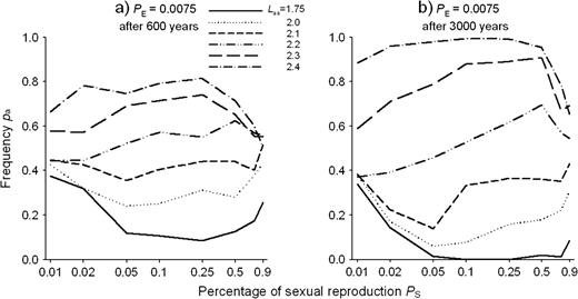
Population frequencies p_a of allele a in a stationary population of the clonal plant after evolution over (a) 600 years and (b) 3000 years for different proportions of sexual reproduction P_S. The gametic SEIB model assumed one locus with two alleles a and A linked to internode length L_V0 by (1). However, values for L_aa, the internode length for the aa homozygotes in a module, varied independent of (1). The values for L_aa are given in the legend. A value of 2.1 corresponds to the case of a symmetric fitness profile. Shown are means from 30 runs. Seedling establishment probability was P_E = 0.0075 and mutation rate 0 for all simulations. The x-axis is log scaled.

Open in new tabDownload slide

Overall, these results of the one-locus gametic SEIB model illustrate that populations of clonal plants with both sexual and vegetative reproduction will deviate, for an asymmetric fitness profile, both from the prediction corresponding to entirely vegetative reproduction of the optimum phenotype (i.e. corresponding to p_a = 0.5) and from the prediction of the CSM of entirely sexual populations (i.e. p_a = 0.125) and that the maintenance of non-optimal genotypes, mutation preventing fixation and the relative importance of sexual reproduction all play a role in shaping p_a.

Evolution in the five-loci gametic SEIB simulation model

Assuming the five-loci gametic SEIB model, the outcome of evolution in the entirely vegetative case (P_S = 0) only slightly deviated from the prediction of the fitness profile of Fig. 1. In 83.3% of all runs, one genotype survived after 3000 years, and only in 16.7% of the cases, a second genotype was still present. In 80% of all cases, only a genotype or a genotype combination with p_a = 0.5 corresponding to the phenotypic optimum (Fig. 1) remained in the final population. However, 16.7% of the runs ended with one or two genotypes with allele frequency p_a = 0.4 and 3.3% of the runs even with p_a = 0.3. Overall, therefore, the mean population allele frequency of all simulation runs after 3000 years was 0.477, i.e. it deviated less from 0.5 than the prediction of p_a = 0.45 by the five-loci CSM.

In contrast to the one-locus case, evolution of the p_a values only slightly depended on the proportion of sexual reproduction P_S (Fig. 6), seedling establishment success P_E (results not shown), evolution period (Fig. 6avs. Fig. 6b) and mutation rate μ (Fig. 6). Nevertheless, similar to the five-loci CSM, the results slightly but consistently deviated from the phenotypic optimum p_a = 0.50.

Figure 6:

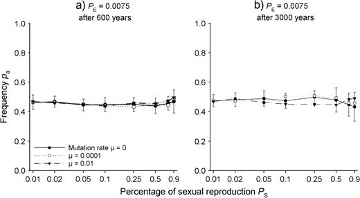
Population frequencies p_a of allele a in the gametic SEIB model after evolution over 600 (a) and 3000 (b) years for different proportions of sexual reproduction P_S and different mutation rates μ assuming five loci with two alleles linked to the internode length L_V0 by (1). Seedling establishment probability P_E = 0.0075. The x-axis is log scaled.

Open in new tabDownload slide

For the five-loci model, hardly any locus was already fixed after 600 years, regardless of the rate of mutations (Fig. 7a). However, after 3000 years and without mutations (μ = 0), a high proportion of loci was fixed (Fig. 7b), in some runs at four or even all five loci. In these cases, we obtained p_a = 0.4 as combination of two fixed aa- and three fixed AA loci, or in some cases also 0.6, which became possible due to the flatness of the profile near the optimum. A mutation rate of μ = 0.0001 reduced the rate of fixation when sexual reproduction was larger than P_S = 0.05, and a mutation rate of μ = 0.01 completely prevented fixation at such proportions of sexual reproduction.

Figure 7:

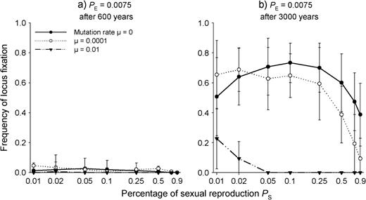
Locus fixation rates for any of the alleles a or A in the five-loci gametic SEIB model after 600 (a) and 3000 (b) years of evolution for different proportions of sexual reproduction P_S and different mutation rates. Seedling establishment probability P_E = 0.0075. The x-axis is log scaled.

Open in new tabDownload slide

Overall, these results illustrate that, compared with populations in the one-locus case, in the five-loci case, populations of clonal plants with both sexual and vegetative reproduction evolve allele frequencies which deviate much less from the prediction derived assuming entirely vegetative reproduction and the phenotypic optimum (i.e. prediction of p_a = 0.5) and from the prediction of p_a derived assuming entirely sexual reproduction and the CSM prediction of (i.e. p_a = 0.45).

DISCUSSION

Fitness profiles

The fitness profile relating stolon internode length to fitness in our study was asymmetric around the phenotypic optimum realized by genotypes with even allele frequency. We think it is highly likely that natural fitness profiles are also asymmetric. Nevertheless, theoretical studies often assume symmetric ones, probably due to the numerical simplicity of, say, parabolic relationships. Much of the deviations of evolving allele frequency from the one expected for genotypes corresponding to the optimal phenotype are due to this asymmetry (Fig. 5). However, even with a symmetric shape, which would remove deviations in the predictions of allele frequencies, the distribution of genotypes coming about due to recombination would still predict the occurrence of many genotypes with phenotypes deviating from the optimal one (Fig. 5).

Of course, in nature different loci have fitness effects of different magnitudes. Therefore, fixation at any locus would cause a deviation from the optimal genotype. However, this mechanism is beyond the scope of our current study.

Studies looking for quantitative trait loci (QTL) report a moderate number of major genes affecting quantitative traits, sometimes only one or two (Stearns and Hoekstra 2000). Therefore, we selected the one-locus and five-loci cases for our gametic models. Of course, because the goal was to study evolution of a certain range of phenotypes, we selected both cases to span the same phenotypic range. It is nevertheless interesting to note that in the five-loci case, many loci went to fixation, which narrowed the phenotypic space actually scanned by the evolving genotypes. This suggests that in nature, genetic variation at QTL is maintained by effects not included in the model, such as spatial heterogeneity between patches, different scales of disturbances or biotic interactions.

Constant selection model

The CSM (2) requires an a priori determination of relative fitness values. Moreover, it explicitly assumes sexual reproduction with segregation and recombination. Therefore, it can only be applied to clonal plants if the clone is treated as the individual and if non-overlapping sexual generations are assumed. However, fitness cannot simply be derived from demographic transition rates for the complex life cycle of clonal plants characterized by a mix of sexual and vegetative reproduction, module and genet (clone) individuals, overlapping generations for both types of individuals and density-dependent and spatially explicit interactions between modules. However, as we showed earlier, for clonal plants, relative fitness of a phenotype realized in competitive situations can be reliably predicted from phenotypic SEIB simulations (Winkler and Fischer 2001). In our context, we used CSM as a reference to investigate deviations from this entirely phenotypic model. These deviations mainly arose due to segregation and recombination, which continuously led to the production of non-optimal genotypes. It must be kept in mind, however, that part of the deviations between the predictions of the phenotypic model and CSM can also be due to the implicit mean-field approximation necessary because of the assumption of constant relative fitness.

In the CSM, fitness profiles become discrete because only a limited number of phenotypes, in our cases 3 or 11, are possible. Asymmetric fitness profiles imply the possibility that the asymmetry around the optimum differs between the cases with more or fewer phenotypes. In our one-locus case, the extreme phenotypes of Fig. 1 differed in fitness by a factor of 3.3, while in our five-loci profiles the three asymmetrically distributed phenotypes at the short-internode and at the long internode ends of the interval differed in fitness only by a factor of 1.21 (weighted according to the number of genotypes corresponding to the phenotypes). This difference in skewness of the finer and coarser discrete fitness profiles explains why the CSM predicts stronger deviations from even allele frequencies for the one-locus than for the five-loci case. Of course, depending on the shape of the fitness profile, a case might arise where predictions of the five-loci model would deviate more strongly than those of the one-locus case. However, we think it is likely that most fitness profiles decrease monotonically, though asymmetrically, from the optimum in both directions, at least locally. Therefore, the higher deviation for the fewer-locus case loci found in our study may well constitute the rule rather than the exception.

Gametic SEIB models

As discussed above, clonal plants deviate from the simplifying assumptions of the CSM. In the CSM, any fitness differences are directly linked to sexual reproduction, whereas in many clonal plants sexual reproduction is relatively rare (Schläpfer and Fischer 1998). Moreover, fitness differences may arise between clonal phenotypes that only differ in vegetative characteristics such as stolon internode length, but not in rates of seed production. Furthermore, even if differences between phenotypes in the number of sexual offspring are large, they may still be of little fitness effect. This is exemplified by Fig. 3, where seedling establishment probability P_E has hardly any effects over large ranges of proportions of sexual reproduction P_S. All these considerations indicate that the CSM is not appropriate to study the evolution of clonal plants. Moreover, because the CSM does not differentiate between sexual and vegetative modes of reproduction, it does not allow for studying the effect of the relative allocation to both modes of reproduction.

The gametic SEIB simulations in the one-locus case deviated the stronger from the predictions of the phenotypic model the higher the degree of asymmetry of the underlying fitness profile was (Fig. 5). Moreover, they deviated from the predictions of the CSM. The gametic SEIB model results may be considered a compromise between those of phenotypic model and CSM, the balance between the two depending on the proportion of sexual reproduction P_S (Fig. 3). This is best explained by the action of two opposing effects. Selection for the optimum phenotype would act to shift allele frequencies towards p_aopt = 0.5. However, with increasing proportion of sexual reproduction P_S, segregation and recombination were more able to shift the evolving allele frequency away from this phenotypic optimum closer to the prediction of the CSM of p_aopt = 0.125 (Fig. 2). This implies that phenotypic models will be able to predict the outcome of selection for organisms with only a very low ratio of sexual to vegetative recruitment. In our example, a proportion of only 10⁻⁴ successful seedling per vegetatively generated module (corresponding to P_S = 0.02 … 0.05 in Figs 3c and d) is sufficient to drive the result towards the CSM prediction.

In the one-locus case, for a high proportion of sexual reproduction P_S > 0.10 and a sufficiently large evolution period, the resulting population allele frequency p_a averaged over many runs not only approached the CSM prediction but also was even lower (Fig. 3). This was due to the fact that the system could approach either of two different stationary states: (i) the state of optimum fitness with a genotype mixture where at least genotype aA was still present, even though with low frequency and (ii) an absorbing suboptimal state with only genotype AA, with only slightly lower population fitness than the optimum state (Fig. 2). Without mutations, this absorbing state constituted an evolutionary trap. The fact that the possibility for genetic drift to such fixation was not negligible is due to the much lower fitness difference of heterozygotes to AA genotypes than to aa genotypes. Of course, mutations of sufficient rate allowed the system to escape this evolutionary trap.

In the five-loci case, both pure phenotypic selection (Fig. 1) and selection under the CSM (Fig. 2) predicted similar allele frequencies of p_a = 0.5 and 0.45, respectively. The latter did not deviate very much from the outcomes of simulations with the full gametic SEIB model and this was not changed by presence or rate of mutations. In this case, the proportion of sexual reproduction P_S had only a small effect on evolving allele frequencies.

In the five-loci case, after 600 years, almost no locus went to fixation in our 70 × 70 cell system. However, after 3000 years, a high percentage of loci was fixed, sometimes four or all five. Partial fixation constrained further evolution, which in the absence of mutations proceeded until complete fixation. However, in contrast to the one-locus case, complete fixation could still result in phenotypes close to the optimum, when some loci were fixed for a and others for A.

CONCLUSIONS

Outcomes of simulated evolution deviated from the phenotypic optimum. This had two major reasons. First, heterozygotes were phenotypically superior to homozygotes. Second, the fitness profile was asymmetric. In nature, this situation may well constitute the rule rather than the exception. Moreover, outcomes of gametic SEIB models also deviated from the predictions of evolution with the CSM, indicating that only gametic SEIB models were able to capture the relevant dynamics. In our example, the deviations between gametic SEIB model and CSM were especially pronounced in the one-locus case because of the stronger asymmetry of the fitness profile. This suggests that the evolution of traits governed by a small number of QTLs will be even less predictable by simple models than the one of traits governed by several or many QTL. We conclude that evolution is considerably constrained by genetic mechanisms and that predictions of phenotypic models and, especially for few loci, also from CSMs need to be interpreted with caution.

Our results imply relevance to the applicability of genetic algorithms in general, i.e. of computational search procedures designed to solve complicated optimization problems in technical and biological contexts (Holland 1975, Sumida et al. 1990; for an ecological application, see e.g. Rose et al. 2002). Such techniques mimic genetic and evolutionary processes and are based on the assumption that in this way optima on fitness landscapes can be found. Our example shows that, when such an algorithm is applied, one has to take care to really meet the optimum of a predefined landscape even in simple cases.

Optimal phenotypes in our situations could better be achieved if they were influenced by allelic variation at several loci of small effect rather than by allelic variation at one locus of larger effect. This suggests that natural selection might favour genetic mechanisms involving many loci with small effects rather than mechanisms with few loci with large effects. It will be interesting to see whether this idea will be confirmed in studies of the molecular nature underlying phenotypic variation in ancestral and derived lines.

Helpful and stimulating comments by Karin Johst and Mark van Kleunen are gratefully acknowledged.

References