


Abstract
Based on Norwegian administrative registers, we provide new empirical evidence on the effects of the childhood neighborhood’s socioeconomic status on early educational performance. A neighborhood’s status is measured annually by its adult inhabitants’ earnings ranks within larger commuting zones, and the childhood neighborhood status is the average status of the neighborhoods inhabited from the year after birth to age 15. Identification of causal effects relies on within-family comparisons only. Our results reveal a distinct hump-shaped relationship between the socioeconomic status of the childhood neighborhood and school results at age 15–16, such that the optimal neighborhood is of medium rank.
1. Introduction
Deciding where to live is among the most important decisions families make over their lifetime. People choose their neighborhood based on a number of factors, such as affordability, proximity to work, school quality, public safety, social networks and social status. These choices then typically lead to a sorting of families closely linked to their earnings; those with high earnings end up in high-earnings neighborhoods whereas those with low earnings end up in low-earnings neighborhoods. Recent empirical evidence shows that this tendency of residential segregation has risen over the past decades both in the USA and Europe, such that neighborhoods have become more homogenous in terms of family income and/or socioeconomic status (Jagowsky, 1996; Bischoff and Reardon, 2013; Marcińczak et al., 2016; Musterd et al., 2017; Reardon et al., 2018). At the same time, existing evidence also indicates that the quality of the childhood neighborhood has a large and potentially long-lasting influence on the educational and economic outcomes of offspring (Crowder and South, 2011; Wodtke et al., 2011; Chetty et al., 2016; Chyn, 2018; Chetty and Hendren, 2018a, 2018b; Chetty et al., 2020). Taken together, these two pieces of evidence point toward a future with growing inequality and lower social mobility.
The purpose of the present paper is to examine empirically how the socioeconomic status of the childhood neighborhood affects early educational performance. Our paper adds to the literature in several ways. First, while much of the existing literature either focus on the impact of moving away from (or into) particularly deprived neighborhoods (e.g. Kling et al., 2007; Clampet-Lundquist and Massey, 2008; Ludwig et al., 2008; Weinhardt, 2014; Chetty et al., 2016; Chyn, 2018), or on effects primarily identified for minority groups (e.g. Damm, 2014; Galster et al., 2016), we examine neighborhood effects across the complete neighborhood status distribution, with a focus on possible non-linearities. This is potentially important, as there is no reason to assume that the marginal effect of, say, moving to a socioeconomically higher-ranked neighborhood is the same (or even has the same sign) throughout the neighborhood status distribution. Second, in contrast to some of the most influential recent studies of neighborhood effects (Chetty and Hendren, 2018a, 2018b; Chetty et al., 2020), the neighborhoods examined in our paper are small and socially homogenous residential communities, with considerable face-to-face interaction among residents. Finally, whereas much of the existing empirical evidence on causal neighborhood effects is derived from US data, we provide evidence from a European welfare state, with considerably less overall economic inequality and smaller differences in the standards of local environments and amenities.
In the main part of our analysis, we use grade point average (GPA) measured at age 15/16 as the primary offspring outcome and we use earnings ranks of the adult population (ages 30–60) to identify a neighborhood’s socioeconomic status. Earning ranks are calculated within commuting zones (CZs) and sex-age-cells, and each neighborhood is characterized in terms of its average inhabitant rank (AIR), with ranks defined in terms of vigintiles (5% bins). While these choices form the basis for the main exposition in this paper, we show that our results are robust with respect to alternative educational and economic outcomes, as well as to alternative neighborhood ranking algorithms. The latter include rankings based on household earnings, household net income (including transfers), male earnings only and educational attainment, respectively.
In line with recent research emphasizing the temporal dimension of neighborhood effects (Crowder and South, 2011; Wodtke et al., 2011; Chetty and Hendren, 2018a, 2018b; Chetty et al., 2020), we focus on the cumulative neighborhood exposure during childhood as the key explanatory variable, measured as the average status of neighborhoods inhabited from the first year after birth to age 15. Throughout the analysis, we use family-fixed effects to eliminate biases following from non-random sorting into neighborhoods. Hence, in essence, we compare full siblings who have been exposed to different neighborhood environments during childhood, either because they have moved residence and/or because the neighborhood they live in has changed. The key identifying assumption is that events associated with changes in neighborhood status affect siblings equally; that is, that their influence does not vary systematically with the age at which they occur. Since the validity of this assumption can be questioned, we assess the consequences of manipulating the sources of identifying variation, both with respect to the ranking of neighborhoods (excluding/including time-variation in individual ranks) and with respect to sources of variation in exposure (excluding/including stayers and movers). We also examine robustness with respect to the inclusion of a wide range of control variables, including the families’ own time-varying earnings ranks. Arguably, we can also sign the expected bias resulting from any remaining unaccounted-for confounding shocks. Based on the plausible assumption that events responsible for raising a family’s neighborhood class are not systematically associated with events that have negative influences on the offspring’s school results, the bias will be positive; that is, it will tend to overstate the positive influence of living in higher class neighborhoods.
Our results reveal a conspicuous hump-shaped and almost symmetric relationship between childhood neighborhood rank and GPA score. Hence, we confirm previous findings that moving upwards from economically disadvantaged neighborhoods contributes to an improvement in offspring educational outcomes. However, the ‘best’ neighborhood to grow up in—in terms of maximizing junior high school GPA score—is a middle-class (medium-ranked) neighborhood. To our knowledge, this important non-linearity has not previously been recognized in the literature. The estimated negative effect of spending childhood in upper-class neighborhoods is statistically significant and robust, both with respect to the choice of specific outcome, with respect to functional form assumptions, with respect to the inclusion of controls for the families’ own social mobility, and with respect to the sources of identification.
2. Data and definitions
Our data contain residential information for all persons living in Norway from 1993 and onwards. Combined with our GPA data, which are recorded by age 15/16 and updated until 2015, we can examine the relationship between childhood neighborhood characteristics and GPA score for all offspring born between 1992 and 1999. Our socioeconomic characterization of neighborhoods is based on the residents’ earnings ranks within larger CZs (travel-to-work-areas). The choice of CZs (rather than the whole country) as the foundation for ranking ensures that rank differences are primarily driven by differences in human capital resources and not by differences in overall economic conditions.
We first divide Norway into 160 different CZs using the classification developed by the Norwegian Institute for Urban and Regional Research, with the purpose of facilitating regional analyses. The division is based on a combination of observed commuting patterns and estimated travel times to regional centers; see Gundersen and Jukvam (2013).1 We then provide a status/class rank to all prime age (age 30–60) individuals living in each CZ. On average, a CZ consists of 11,938 prime-age individuals, but the variation is large, from less than hundred in the smallest isolated islands to around 600,000 in the capital area. Hence, the population-weighted mean is much larger than the unweighted mean, and the average person lives in a CZ with 160,000 adults; see Figure 1(a) for a description of the population-weighted size distribution.
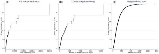
The cumulative population-weighted size distributions of CZ and neighborhoods in Norway.
Notes: Size is measured by the number of adult (age 30–60) residents. The data points in (a) and (b) correspond to the 160 CZs, whereas the data points in (c) correspond to the 12,640 neighborhoods included in our analysis.
The economic ranking of individuals is done separately for each year from 1993 through 2015 on the basis of observed labor earnings. In our baseline specification, all residents between age 30 and 60 are assigned a vigintile rank based on their position in the CZ’s age- and gender-specific distribution of labor earnings. Hence, each person is for each calendar year attributed a rank number from 1 to 20, describing his/her earnings rank relative to all others of the same age and sex living in the same CZ.2 The choice of individual (age-specific) earnings as the primary ranking criterion is motived by the argument that Norway is a country where there is a strong labor market participation norm, with similar labor force participation rates for men and women, and little evidence for widespread within-household specialization based on relative earnings (Raaum et al., 2008). However, our results are robust with respect to a wide range of alternative ranking criteria, based on, for example, male earnings only, household earnings, household net income and educational attainment, and also robust with respect to ranking within wider age groups and within all adults.
The CZs are further divided into neighborhoods. The neighborhoods used in our analysis correspond to the ‘basic statistical units’ defined by Statistics Norway for the purpose of providing an efficient statistical foundation for analyses and local and regional policy planning. According to Statistics Norway (1999), the main criteria used to define the basic units are that they constitute a coherent and connected geographical area, that they are stable over time, and that they are homogenous with respect to the natural environment, communications and the type of housing and building structure.
Having established individual ranks within CZs, we characterize each neighborhood in terms of its AIR. On average, a CZ consists of 79 neighborhoods with an average number of 152 prime-age residents. Again, the variation is large, and the average inhabitant lives in a CZ with 704 neighborhoods, and in a neighborhood with 322 prime-aged residents; see Figure 1(b, c) for a description of the population-weighted size distributions. The smallest CZs have just a single neighborhood (implying that they will have no role to play in our empirical analysis), whereas the largest have approximately 2,000 neighborhoods. And the neighborhood size varies from just 10 prime-age residents in the smallest to 2,800 in the largest.3
In order to examine the influence of the childhood neighborhood on offspring outcomes, we follow Ginther et al. (2000), Crowder and South (2011), Wodtke et al. (2011) and Chetty and Hendren (2018a, 2018b) in that we focus on the impact of accumulated exposure to different local environments during childhood and adolescence, and not on the environment experienced at a particular point in time. We thus compute the average neighborhood rank exposure for each offspring as the weighted average of the neighborhood inhabitant rank (leaving out the offspring’s own parents) he/she has been exposed to, such that each age 1,…,15, is attributed a weight of 1/15. The resultant variable thus indicates the average neighborhood inhabitant rank, an individual has been exposed to over the complete period from the year after birth to age 15.4
Our primary outcome variable is going to be the GPA from junior high school (lower secondary education), typically measured at age 15–16, during the last year of compulsory school. GPA is computed as the average grade (on a scale from 0 to 6) obtained in all subjects, and includes both final assessment and national exam grades. As the key explanatory variable is defined in terms of ranks within CZs, we also define the GPA outcome in terms of rank (percentile) in the distribution of GPA scores within the same zones. This makes it easier to interpret the estimated effects and has the advantage that the marginal distribution of the outcome is by construction the same across CZs and years. Toward the end of the paper (Section 6), we present some additional results based on educational and economic outcomes measured later in life; that is, (i) an indicator variable for completed high school (upper secondary education) by age 21, (ii) the number of non-compulsory education years attained by year 2020 and (iii) labor earnings at age 30–32. The latter outcome is not yet available for the 1992–1999 cohorts; hence, this particular analysis is based on the 1980–1987 cohorts instead, with neighborhood status during adolescence () as the explanatory variable of interest.
3. Why neighborhoods matter
Characteristics of the childhood neighborhood may influence adolescent and adult outcomes through a number of channels; see, for example, Harding et al. (2011), Sharkey and Faber (2014) and Graham (2018) for recent overviews of the literature. The causal effects fall into two main categories, those related to the characteristics of the neighborhood itself and those related to the people living there. The first category comprises factors like the physical environment (air and water quality, traffic noise, access to parks and playgrounds), public amenities (quality of schools and childcare facilities) and infrastructure. The second comprises the quality of the social environment, the existence of good and bad role models and other peer influences.
Although the AIR metric outlined in the previous section describes the people living in a neighborhood rather than its amenities and environment, it may be correlated with the latter factors, as wealthier people are likely to choose neighborhoods with higher standards. However, as our analysis is conducted within a welfare state more or less designed to equalize living conditions across neighborhoods, we expect the differences in these conditions to be much smaller than in, say, a US context; see, for example, Borge (2010, 2013) for a description of equalization mechanisms in the Norwegian system for allocation of resources across local governments.
A potentially important source of neighborhood influence on educational performance is the choice of primary and lower secondary school. The vast majority of Norwegian children attend their local school; hence, children from the same neighborhood typically also attend the same school. However, the neighborhoods examined in this paper are much smaller than the school districts, and many school districts cover neighborhoods with quite different socioeconomic statuses. The average (median) number of neighborhoods belonging to a junior high school’s catchment area is 13.1 (11), and the average (median) inhabitant rank distance between the highest and the lowest ranked neighborhood belonging to the same catchment area is 3.5 (3.4). School resources are allocated in a way that appears to be inversely related to the neighborhood ranks of pupils. Based on the data described in the previous section and data on the number of employees at each junior high school (collected from the Norwegian employer-employee register), we show in Online Appendix A that there is a significant negative relationship between the school’s teacher-student ratio and the students’ neighborhood rank. This does not necessarily imply that schools in lower-class areas provide a better learning environment, however, as the extra resources are intended to compensate for a more disadvantaged composition of students.
Although neighborhoods are characterized in terms of the neighbors’ earnings rank, we do not think of the earnings themselves as the primary causal factor. Rather, we think of earnings rank as a proxy for a number of potentially important peer attributes, such as parenting style, cognitive and social ability, educational attainment, self-control, aspirations and work morale. We know from existing evidence that parental earnings rank is positively correlated with educational and economic outcomes in the offspring generation (Chetty et al., 2014, Pekkarinen et al., 2017; Markussen and Røed, 2020); hence, we expect that neighborhoods with high average earnings ranks are also characterized by high average levels of human capital, both in the parent and offspring generations. This implies that children growing up in upper-class neighborhoods tend to have peers with more human capital than children growing up in lower-class neighborhoods.
There is a large existing literature on neighborhood effects covering a wide range of outcomes, from physical and mental health to criminal behavior to education and adult earnings. Yet, according to a comprehensive survey by Oakes et al. (2015), there is little consensus on the nature and direction of the effects, and the vast majority of contributions fail to deal with the most fundamental identification problems. With respect to peer influences on academic achievement, there is also an extensive literature focusing on the social interaction within classrooms. A typical finding in this literature is that higher-achieving peers have moderate beneficial effects on most pupils, yet with considerable effect heterogeneity; see, for example, Sacerdote (2011) and Epple and Romano (2011) for overviews.
Within the psychology literature, a prevalent finding is that higher-achieving peers have negative ‘relative deprivation’ effects on academic self-concept and academic achievement, and this phenomenon has been labeled the big-fish-little-pond effect; see, for example, Marsh (1987) and Marsh and Hau (2003). Similar results have also recently been reported in the economics literature. In particular, it has been shown that higher ordinal ability rank within a school cohort improves test scores (Murphy and Weinhardt, 2020), reduces risky behaviors, and raises expectations regarding own educational achievement (Elsner and Isphording, 2018). The finding of negative influences of higher-achieving peers has a long tradition within a literature discussing what is known as the ‘relative age effect’. This label refers to the age variation occurring within grade cohorts in education and sports due to the use of a single cutoff date for enrolment into age-specific groups. Based on the resultant presumed random-assignment-like source of within-group age variation, it has been shown that the oldest members of the groups have been given a lasting advantage, both in education (Bedard and Dhuey, 2006) and in sports (Barnsley et al., 1992; Allen and Barnsley, 1993; Delorme et al., 2010; González-Villora et al., 2015). The existence of a lasting advantage in education is questioned, however, by Black et al. (2011), who find no evidence of a long-term effect of school starting age on education and earnings in Norway.
4. Sources of identification and graphical evidence
In the raw data, there is a strong positive correlation between neighborhood rank exposure and GPA percentile rank; see Online Appendix B. Offspring growing up in upper-class neighborhoods do systematically better. This does of course not provide any evidence of causality. As we expect massive selectivity in the sorting of families into neighborhoods with different ranks, we base the causal analysis on sibling comparisons only, as originally pioneered in this setting by Aaronson (1998). Identification thus comes from families with at least two children born between 1992 and 1999, where the children have been exposed to varying neighborhood characteristics, either because they have moved or because the neighborhood they live in has changed. This leaves us with 227,202 observations divided between 106,099 families.
Figure 2(a) shows the distributions of childhood neighborhood ranks in the population and in the sibling sample. The two distributions are hardly distinguishable, suggesting that there are no external validity problems related to the use of siblings data. The majority of offspring in our data grew up in middle-class neighborhoods, with close to 10.5 (the value corresponding to random assignment of individuals across neighborhoods). These offspring typically also grew up in diverse neighborhoods. Using the expected earnings rank distance between two randomly chosen adults in a neighborhood as a measure of diversity, we find that offspring with between 10 and 11 on average had been exposed to a rank distance of 6.4, close to what we would have seen under random assignment.5

The distribution of for all offspring in the siblings data (a) and the corresponding sibling differences (b).
Notes: The number of observations in the total sample is 429,919. Number of observations in the sibling data (estimation sample) is 227,202 divided between 106,099 families. Panel (b) shows the distribution of all calculable sibling differences (youngest minus oldest). For example, in a family with four children, there will be six such differences (#2-#1, #3-#1, #4-#1, #3-#2, #4-#2 and #4-#3).
Figure 2(b) presents the variation in that can actually be exploited in the causal analysis, namely the distribution of within-family differences. It reveals that the foundation for identification is limited, as the difference in between siblings rarely exceeds 1. It also indicates a slight asymmetry, in the sense that it is more common that the youngest sibling experience the highest than vice versa.
Figure 3 gives a descriptive overview of the relationship between siblings’ differences in and their differences in GPA rank. Panel (a) contains a binned scatterplot showing, for all sibling pairs, the mean difference in GPA score between the youngest and the oldest sibling by the corresponding difference in their (with bin size equal to 0.02). Although there appears to be a slight negative relationship between the difference in and the difference in GPA within families, the association is weak and statistically insignificant.6 The main takeaway from Panel (a) is that of a non-existing systematic relationship. However, if neighborhood effects are non-linear, such that the impact of sibling differences in neighborhood exposure depends on the location of the change, Panel (a) might well conceal a causal relationship. It appears plausible that, say, moving upwards from a very poor neighborhood has a different effect than moving upwards from an already rich neighborhood.
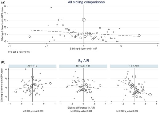
Sibling differences in schooling outcome (GPA) and neighborhood rank .
Notes: Panel (a) shows a binned scatterplot of the relationship between sibling differences in AIR (youngest minus oldest) and the corresponding differences in GPA score. Bin size is 0.02 between −0.5 and +0.5, with the bottom and top data points including all observations below and above these thresholds, respectively. Circle sizes are proportional to the fraction of observation in each bin. Panel (b) is constructed in the same way, with sibling pairs sorted into the different panels according to their average AIR. The dashed lines are linear regression lines (weighted by the number of observations in each bin), and slope coefficients are reported below each line with p-value.
To assess the case for non-linearity, we divide in Panel (b) the sibling pairs into three groups, by their average A more illuminating pattern emerges: At low levels of , a positive difference is associated with improved GPA rank, whereas at high levels of , the same difference is associated with reduced GPA rank. While the former of these effects is borderline statistically significant (p = 0.093), the latter is highly significant (p = 0.003). In the middle, there appears to be no effect at all. In Panel (a), these positive and negative influences apparently cancel out, concealing the underlying systematic relationship.
The use of sibling comparisons to identify causal neighborhood effects implies that our analysis will not be biased by any systematic sorting into neighborhoods based on stable family characteristics. However, we cannot rule out confounders generated by events that influence both a family’s neighborhood quality and their offspring outcomes. There are essentially three sources of identification in our data: (i) families who move to a new neighborhood, (ii) families who stay in the same neighborhood, but are exposed to changed neighborhood status due to in- and outmigration of others and (iii) families who stay, but are exposed to changed neighborhood status due to economic mobility of existing neighbors. These sources of identification represent different levels of intervention, where the movers have been subjected to a family-level intervention, whereas the stayers have been subjected to a neighborhood-level intervention; see Sampson (2008) for a discussion of neighborhood effect interpretations in this context.
Each source of variation in raises distinct concerns regarding possible confounders. For example, a move to a new neighborhood can be triggered by a wealth shock, a job loss or a divorce; and such events may have different direct effects on offspring depending on their age. A change in the rank of an existing neighborhood can be triggered by local events such as a major plant closure or the establishment of new employment opportunities, which again may affect siblings differently. It is thus of interest to see how each source of variation in contributes to identification of estimated neighborhood effects.
As a first step toward setting up a causal statistical model, we divide the sibling pairs into a large number of bins based on each pair’s average . We then estimate the marginal effect of on GPA score separately within each bin by means of linear regressions. With almost all sibling-pair-averages located between 7.5 and 13.5 and with a bin size equal to 0.1, we obtain 66 such bins and a corresponding number of estimated slope parameters. Figure 4 plots these 66 marginal effect estimates against the siblings’ average levels of , together with a (weighted) regression line through the points. Panel (a) shows the results for the complete sibling sample, whereas Panels (b)–(d) show results for each of the three identification sources separately. Although there is much noise in these estimations, it seems clear that the estimated marginal effects display a tendency to decline systematically with the level of regardless of identification source.
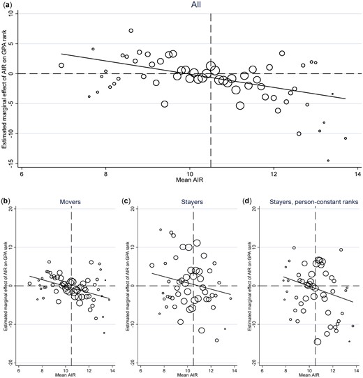
Estimated marginal impacts (point estimates) of neighborhood rank exposure on GPA score by the siblings mean .
Notes: Each data point in Panel (a) is the estimated slope parameter from bin-specific regressions of the following kind: where the differences are taken within siblings (youngest minus oldest). There are 66 bins of size 0.1, and the sizes of the circles are proportional to the fraction of observations behind each regression. The solid line is a weighted regression line through the 66 data points. Panels (b)–(d) show the corresponding statistics based on different identification sources. Panel (b) is based on families who move at least once during the observation period (# of siblings = 155,447). Panel (c) is based on families who do not move (# of siblings = 71,755). Panel (d) is based on the same sibling pairs as Panel (c), but with neighborhood ranks calculated from person-constant ranks. These ranks are computed as the average earnings rank obtained for each person; see Online Appendix D for details.
5. Parametric regression analysis
Based on the descriptive patterns laid out in the previous section, it is clear that a parametric regression model aimed at statistical inference has to take the potential non-linearity of the relationship between and GPA rank into account. In its simplest form, we estimate the following baseline model: where is the GPA score percentile rank (in the CZ) for offspring i belonging to family j, and born in year t, is some unknown function, is a family fixed effect, is a birth-year fixed effect, and BO and GENDER are birth-order- and gender-fixed effects, respectively.7 In the context of Equation (1), identification of the effects of requires that the residual term is uncorrelated with the included terms, conditional on the family fixed effect and the other control variables. The plausibility of this assumption may vary somewhat across the sources of identification, and it is arguably less disputable for stayers (who have been exposed to a neighborhood-level intervention) than for movers (who have been exposed to a family-level intervention). An important point to note, however, is that as long as unaccounted-for shocks that are favorable to offspring outcomes raise the probability of moving to (or staying in) a higher-ranked neighborhood, whereas adverse shocks raise the probability of residing in a lower-ranked neighborhood, the omission of such shocks imposes a positive bias on the impact of ; that is, in the context of Equation (1), they will imply that
We begin by estimating alternative versions of Equation (1), where we represent the effects of thorough polynomial or spline functions. Results for the full sample are displayed in Figure 5(a), where we have used polynomials from degree one to three, plus linear and cubic splines. Within the range of actual support (note the vertical lines marking the 1st and 99th percentiles of the distribution; see also Figure 2), the estimated impact of neighborhood rank () follows a distinct quadratic pattern. All the non-linear specifications form an almost symmetric concave relationship between neighborhood rank and GPA rank, with the best outcome obtained when growing up in medium-ranked neighborhoods. Panels (b)–(d) show the estimated effect profiles based on the three different sources of identification discussed in the previous section. A second-order polynomial fits the data well regardless of identification source.
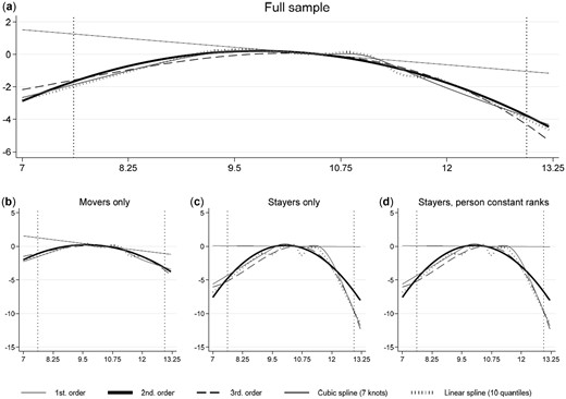
The estimated impacts of neighborhood rank exposure on GPA score percentile with alternative polynomial and spline functions and alternative sources of identification.
Notes: The linear and cubic spline functions are computed with the mkspline command in Stata and the location of knots for the cubic spline are determined by the percentiles recommended in Harrell (2001). Panel (a) shows the estimated functions from Equation (1) with measured on the horizontal axis. Panels (b) and (c) show the same for families who move at least once and families who don’t move during the observation period, respectively (# siblings equal to 155,447 in the mover-sample and 71,755 in the stayer-sample). Panel (d) shows the results for stayers, but with neighborhood ranks calculated from person-constant ranks; see note to Figure 4. The vertical dotted lines indicate the first and 99th percentile in the full sample distribution of located at 7.6 and 12.9, respectively.
Although the estimated hump-shape appears to be more accentuated in the stayer than in the mover sample, it is important to bear in mind that the identifying variation in neighborhood rank is heavily concentrated in the middle of the rank distribution, implying that the statistical uncertainty regarding these functional forms is considerable. The difference between the two estimated second-order polynomials shown in Panels (b) and (c) is thus not statistically significant (p-value: 0.63). To ensure sufficient power, we build our discussion of the main results and the subsequent robustness analyses on the full sample. We return to additional separate analyses for movers and stayers in Online Appendix C, including separate analysis for movers moving upwards and downwards, and stayers staying in upwards-moving and downwards-moving neighborhoods. In Online Appendix D we provide, both for the complete sample and for movers and stayers separately, an analysis where we re-rank neighborhoods based on fixed individual inhabitant earnings ranks only (defined as the average rank obtained for all available earnings years). These different exercises show that our main findings are robust with respect to which of these sources that forms the basis for identification, except for movers moving downwards where we do not find any significant effects.
Given the large variation in the sizes of Norwegian neighborhoods (conf. Figure 1), a possible concern is that the identifying variation in neighborhood status within families is dominated by very small neighborhoods—for which AIR may be influenced by just a few movements into or out of the neighborhood. In Online Appendix E, we provide a separate analysis for families who have never lived in a ‘small’ neighborhood, varying the definition of ‘small’ from below 50 to below 200 adult inhabitants (the latter implies that we drop 63% of the observations). The results show that our main findings are robust with respect to the neighborhood size distribution. If anything, the finding of a concave relationship between neighborhood status and GPA score becomes even clearer when we zoom in on families who have lived in larger neighborhoods.
Based on the finding of a concave functional form relationship in the relevant area of actual neighborhood rank support, we present in Column I of Table 1 the estimated parameters following from a baseline model which is quadratic in . Both the linear and the quadratic terms are statistically significant. The resultant profile of marginal effects is shown in Figure 6 as the baseline (solid bold line), with a 95% confidence interval. It is notable that this line is remarkably similar to the marginal effect profile based on 66 separate regressions displayed in Figure 4(a), above. While there are considerable positive impacts of moving to higher-ranked neighborhoods from the bottom part of the neighborhood rank distribution, there are at least as large negative effects at the top. The turning point is located at the center of the distribution; hence, the optimal childhood neighborhood (in terms of maximizing GPA score) appears to be a medium one, with average rank around 10–11.
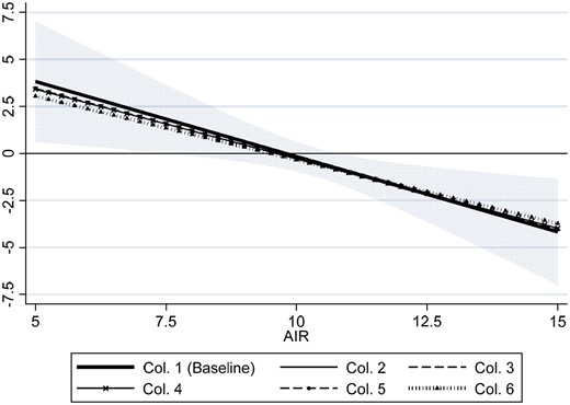
Estimated marginal impact of neighborhood rank exposure on GPA score percentile with 95% pointwise confidence intervals for the baseline model.
Note: Column numbers refer to the columns in Table 1.
Estimated effects of neighborhood rank exposure on GPA score rank (within CZ) at age 15/16 (standard errors in parentheses)
| I (Baseline) | II | III | IV | V | VI | |
|---|---|---|---|---|---|---|
| Neighborhood rank | 7.812*** (3.101) | 7.815*** (3.100) | 7.855*** (3.102) | 7.113** (3.125) | 7.211** (3.150) | 6.434** (3.138) |
| Neighborhood rank squared | −0.400*** (0.149) | −0.399*** (0.149) | −0.398*** (0.149) | −0.370** (0.148) | −0.375** (0.150) | −0.339** (0.148) |
| Own parents’ (time-varying) rank | −0.132 (0.138) | −0.129 (0.138) | −0.130 (0.138) | −0.125 (0.139) | −0.126 (0.139) | |
| Avg. earnings rank of schoolmates’ parents | −0.661*** (0.144) | −0.733*** (0.146) | −0.699*** (0.180) | −1.191*** (0.170) | ||
| Immigrant share among schoolmates | −3.366** (1.562) | −2.925 (1.820) | −2.951* (1.669) | |||
| Immigrant share among neighbors | −5.506 (7.519) | −5.228 (7.570) | −5.518 (7.274) | |||
| School-fixed effects | No | No | No | No | Yes | Yes |
| Avg. GPA score rank among schoolmates | 0.252*** (0.024) | |||||
| N | 227,202 | 227,198 | 227,198 | 227,198 | 227,166 | 227,057 |
| R2 | 0.7551 | 0.7551 | 0.7552 | 0.7552 | 0.7591 | 0.7598 |
| R2 adjusted | 0.5405 | 0.5405 | 0.5406 | 0.5406 | 0.5432 | 0.5445 |
Notes: All models include family fixed effects and also contain controls for within-family birth order (six dummy variables), birth-year (seven dummy variables) and sex. Standard errors are clustered at the school level. */**/*** indicates statistical significance at the 10/5/1% levels.
To interpret the magnitudes of the estimated marginal effects, recall that is measured in vigintiles, whereas GPA rank is measured in percentiles. Hence, for example, the marginal effect approximately equal to 2 at implies that moving at birth from such a low-class neighborhood to a neighborhood where the adult population on average is ranked 1 vigintile higher improves the GPA rank by 2 percentiles, ceteris paribus. Correspondingly, the effect close to −2 at implies that the same upwards movement from such a high-class neighborhood reduces the GPA rank by 2 percentiles.
We now explore how the estimated neighborhood effects change as we add in a range of contextual control variables in a step-by-step fashion; see Table 1, Columns II–VI, with graphical illustrations of the implied marginal effect profiles in Figure 6. As discussed above, our identification strategy may be threatened if siblings exposed to different neighborhoods have also been exposed to different family circumstances in a way that confounds our estimated neighborhood effects. To assess the empirical relevance of this concern, we add into the model a control for the parents’ own time-varying socioeconomic status. This is done in the same fashion as for the neighborhood ranks, such that for each offspring, we compute the parents’ average annual (age-specific) vigintile earnings rank (within the CZ) during the offspring’s age 1–15. The result from this exercise is presented in Table 1, Column II. It indicates that the time-varying parental rank variable has no effect on the offspring GPA outcome, and that the inclusion of this variable does not change the estimated neighborhood effects.
One potential mechanism behind the neighborhood effect is that the choice of neighborhood in practice determines the choice of school, and through that also the composition of schoolmates. In our data, as much as 87% of the siblings attend the same junior high school, however, hence most of the identifying variation in neighborhood exposure is within-school-districts.8 Still, the composition of classmates may vary within schools from year to year, and to examine this potential contextual effect, we add into the model control for the average earnings rank of the schoolmates’ parents.9 In doing so, we first compute each parent’s average earnings rank taken over years with offspring in the dataset, and then compute the average of the resultant variable at the school-year-level. The estimated impacts of the childhood neighborhood remain the same, suggesting that the composition of junior high school classmates is not an important factor behind the identified neighborhood effects; see Column III. Still, it is notable that the prevalence of higher-ranked co-students is estimated to have a significant negative effect on own achievement, confirming that higher relative position within a group is beneficial also in a classroom setting.
Another potentially important contextual factor is the residential pattern of immigrants. A neighborhood’s socioeconomic class is closely related to its fraction of immigrants from low-income countries. In our data, the fraction of immigrants from developing countries and Eastern Europe declines rapidly with a neighborhood’s socioeconomic status through the lower half of the neighborhood rank distribution, from around 40–50% in the lowest ranked neighborhoods to less than 10% in middle and upper-class neighborhoods. There is a literature indicating that the learning environment within schools may be affected by the fraction of immigrant (or foreign language) students; see, for example, Ohinata and van Ours (2013) and Diette and Oyelere (2017). Hence, a natural question to ask is whether neighborhood effects identified here pick up some effects of being exposed to immigrants. In Column IV, we report estimation results from a model where we also control for exposure to immigrants from low-income countries, both among neighbors during childhood (defined in exactly the same way as only with the neighborhood’s immigrant share instead of income rank), and among schoolmates. The point estimates indicate a negative influence of high immigrant exposure, and for schoolmates the effect is also statistically significant at the 5% level. However, controlling for these variables does not alter either the estimated impact of neighborhood rank or the estimated impact of the schoolmates’ class background.
School choice may influence GPA, not only due to peer composition, but also due to variation in school quality (e.g. related to the compensating resource allocation described in Section 3) and differences in GPA standards. In particular, it is possible that teachers’ GPA standards to some extent are adjusted to student composition, such that it is easier to obtain a high GPA score in a school with low overall student performance. A systematic relationship between neighborhood rank and school quality or GPA standards does not invalidate the causal nature of the estimated neighborhood effect. Regardless of its source, a student’s GPA score has important real consequences, as it may determine whether a desired upper secondary education becomes a reality. However, it does induce some ambiguity to its interpretation. To sort out neighborhood effects operating through school quality or grading standards, we add school-fixed effects into the model (Column V) and the average GPA score rank among schoolmates (Column VI). The latter variable is subject to a reflection problem (Manski, 1993), as the schoolmates both affect and are affected by the focal individual, making it difficult to interpret the estimated coefficient. However, in our setting it serves primarily as an extra control variable. As it turns out, neither the inclusion of school-fixed effects nor the added control for schoolmates’ GPA score appear to change the estimated neighborhood effects to any noticeable extent.
While we have identified a hump-shaped relationship between childhood neighborhood rank and GPA score, we have entered all the control variables linearly, including the rank of schoolmates’ parents. This choice is convenient in the sense that it makes it easier to interpret the estimated coefficients. However, it is also supported by the data. In Online Appendix F, we report estimates based on models in which all the control variables enter through quadratic terms. As can be seen there, none of the added second-order terms are significantly different from zero, and their inclusion does not noticeably change the estimated impacts of neighborhood rank.
Our empirical strategy relies on the idea that neighborhoods are appropriately ranked on the basis of their adult men’s and women’s age-specific earnings rank within CZs. It is possible to argue for alternative ranking algorithms. For example, assortative mating may imply that some persons (typically women) have low earnings, not because they have low human capital, but because they share household with a rich spouse. We have thus re-estimated our (baseline and full) model based on a number of alternative ranking criteria: (i) based on male earnings only, (ii) based on household earnings, (iii) based on household net income and (iv) based on educational attainment. In addition, we have re-estimated the models based on rankings within wider (10-year) age ranges and also without age and gender cells at all. The results from these exercises are presented in Online Appendix G. They show that our main conclusions are robust with respect to the choice of ranking criterion.
Throughout this section, we have assumed that the neighborhood effects are appropriately represented by total exposure during age 1–15, and that they are independent of gender and on own family background. In Online Appendix H, we present estimates from less restrictive models; that is, we allow different phases of childhood to differ in importance, and we also allow the effects to vary by sex and own family background. The results indicate that the effects are similar both across childhood phases and gender, although they point toward somewhat larger effects for girls than for boys, and that the neighborhood influence is largest during the junior high school period. With respect to own class background, the evidence points toward larger effects for middle and upper-class offspring.
6. Educational and economic outcomes at higher age
Given that GPA standards may respond to student composition (such that GPA does not fully reflect learning), it is of interest to examine outcomes that capture subsequent educational achievements also. The existing literature shows that skills accumulated in early childhood are complementary to later learning (Cuhna et al., 2006); hence, it is probable that the effects identified for junior high school performance persist into higher ages. Our data contain educational attainment records up to and including the year 2020; hence, we can follow all the birth cohorts included in our analysis (1992–1999) to (at least) age 21. This makes it possible to check whether an upper secondary education has been completed within reasonable time (normal progression implies completion by age 19 or 20, depending on track, and, in our data, 78.2% has completed by age 21).
Columns I and II of Table 2 show results when we use high school completion by age 21 as a dichotomous outcome. We focus on the baseline specification and the model with all control variables included, that is, the models corresponding to Columns I and VI in Table 1. Estimated marginal effects from the baseline specification are reported in Figure 7(a). Whereas point estimates indicate a hump-shaped relationship between and high school completion, again with around 10.5 offering the best chances, the statistical uncertainty is too large to reject other functional forms. We suspect that the information content in the dichotomous completion outcome is too small to facilitate sufficiently precise causal identification. The vast majority of siblings (71.4%) has the same high school completion outcome, and given that we use family-fixed effects, these siblings cannot contribute to identification at all. To squeeze more information out of the data, we thus exploit records on years of educational attainment by 2020 (the last available year with educational information in our data) for all the cohorts in our dataset, realizing that this introduces an asymmetry such that earlier birth cohorts are observed at higher ages than later cohorts. The inclusion of cohort-fixed effects ensures control for the resultant differences in average attainment across cohorts. The results, shown in Table 2, Columns III and IV and in Figure 7(b), indicate a highly significant concave relationship between and years of education.
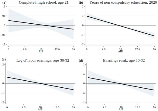
Estimated marginal impact of neighborhood rank exposure on educational and adult economic outcomes with 95% pointwise confidence intervals.
Note: The reported marginal effects build on the baseline models; see note to Table 2 for details.
Estimated effects of childhood/adolescence neighborhood rank exposure on educational and earnings outcomes (standard errors in parentheses)
| High school graduation by age 21 | Years of education by age 21–28 | Log(labor earnings) | Earnings rank | |||||
|---|---|---|---|---|---|---|---|---|
| Age 30–32 | Age 30–32 | |||||||
| I | II | III | IV | V | VI | VII | VIII | |
| Baseline | All controls | Baseline | All controls | Baseline | All controls | Baseline | All controls | |
| Neighborhood rank | 0.049 (0.061) | 0.045 (0.063) | 2.016*** (0.314) | 2.011*** (0.324) | ||||
| Neighborhood rank squared | −0.002 (0.003) | −0.002 (0.003) | −0.104*** (0.015) | −0.104*** (0.015) | ||||
| Neighborhood rank | 0.132* (0.069) | 0.127* (0.068) | 0.636* (0.372) | 0.572 (0.373) | ||||
| Neighborhood rank squared | −0.007** (0.003) | −0.007** (0.003) | −0.033* (0.018) | −0.031* (0.018) | ||||
| Own parents’ (time-varying) rank | −0.002 (0.003) | −0.069*** (0.013) | ||||||
| Avg. earnings rank of schoolmates’ parents | 0.001 (0.003) | 0.006 (0.017) | ||||||
| Immigrant share among schoolmates | 0.002 (0.030) | −0.060 (0.161) | ||||||
| Immigrant share among neighbors | −0.038 (0.131) | −0.037 (0.663) | ||||||
| Avg. GPA score rank among schoolmates | 0.000 (0.000) | −0.001 (0.002) | ||||||
| School-fixed effects | No | Yes | No | Yes | No | No | No | No |
| Birth-year-by-commuting-zone fixed effects | No | No | No | No | No | Yes | No | Yes |
| N | 227,202 | 227,057 | 227,202 | 227,057 | 197,915 | 207,433 | 207,433 | 197,915 |
| R2 | 0.5996 | 0.6056 | 0.6742 | 0.6786 | 0.619 | 0.622 | 0.622 | 0.619 |
Notes: The results reported in Columns I–IV are based on the 1992–1999 birth cohorts, whereas the results in Columns V–VIII are based on the 1980–1987 cohorts. All models include family fixed effects and controls for within family birth order (six dummy variables), birth-year (seven dummy variables) and sex. In Columns I–IV, standard errors are clustered at the school level. In Columns V–VIII, standard errors are clustered at the commuting-zone-by-year level. */**/*** indicates statistical significance at the 10/5/1% levels.
To examine outcomes at even higher ages, we obviously need to look at sibling cohorts born before 1992–1999. The price we have to pay for this is that we will have less than complete information about the neighborhoods inhabited at very low age (as residential information is available from 1993 only). However, as we show in Online Appendix H, the neighborhoods inhabited during junior high school seem to be of particular importance; hence, it is arguably of interest to see how adult outcomes depend on the socioeconomic status of neighborhoods inhabited during adolescence. To shed some light on longer-term effects, we thus use data for the 1980–1987 birth cohorts to examine the causal relationship between neighborhood rank experienced during age 13–15 and labor earnings obtained at age 30–32 (adjusted for aggregate wage growth). We specify two different outcomes based on age 30–32 earnings:10 (i) log(average annual earnings), excluding zero-observations (4.6% of the sample) and (ii) earnings rank (compared with other members of the same birth cohort who grew up in the same CZ).
The statistical approach is the same as in the baseline GPA model above; that is, we use family fixed effects, birth-year fixed effects and controls for birth order and gender. In addition, in a ‘full model’ we control for commuting-zone-by-birth-year fixed effects.11 Estimation results are reported in Table 2, Columns V–VIII, with marginal effects displayed in Figure 7(c, d). Both models estimate a hump-shaped relationship between neighborhood rank and adult earnings, with statistically significant second-order terms.
7. Concluding remarks
We have provided evidence that there is a distinct hump-shaped causal relationship between the socioeconomic rank of childhood neighborhoods and early educational performance. While we have used GPA rank from junior high school as the primary outcome, we have also shown that the hump-shaped effects persist into later educational achievements and adult earnings. It is a robust result that the best expected performance is achieved when growing up in middle-class neighborhoods. Our findings imply that residential segregation may be harmful for offspring from all classes, with a possible exception for offspring from the very bottom of the class distribution. However, segregation does not necessarily increase the inequality between high and low-status offspring. Our results therefore turn upside down the popular notion that while segregation is certain to increase inequality, it has indeterminate effects on average child development; see, for example, Mayer (2002).
The analysis provided in this paper cannot be used to sort out exactly what kind of mechanisms that are behind the identified neighborhood effects. Based on the existing literature, we hypothesize that the favorable effects of moving from low to middle-class neighborhoods reflect positive peer influences arising from socializing with people who are resourceful in terms of human capital and family support, and of being less exposed to children and adolescents with social and behavioral problems. The adverse effect of moving even further up in the neighborhood hierarchy may reflect the negative relative deprivation effect of experiencing a declining relative position, which can arise both due to lower attention from peers and teachers and due to lower self-confidence and educational ambitions.
While it seems probable that the choice of primary and junior high school is an important mediator of neighborhood influences, our results speaks against school choice as the dominating mechanism. The estimated hump-shaped effect of childhood neighborhood status remains almost unchanged when the analysis controls for school-fixed effects and the socioeconomic composition of schoolmates in the final year of junior high school.
Our results are relevant for parents making residential decisions with an eye to possible consequences for their offspring, and the main takeaway for them is that the widespread view that it is best for the kids to grow up in wealthy neighborhoods may be misplaced. Our results are also of relevance for city planners and developers making decisions about new housing projects. The finding that neighborhoods with a representative socioeconomic composition provide the best environment for child development suggest that neighborhoods can benefit from having a diverse housing standard, allowing people from different classes to live together. According to our results, offspring from both lower and upper-class families could benefit from living together in the same neighborhoods instead of segregating into lower and upper-class neighborhoods.
The identification of a hump-shaped causal relationship between the socioeconomic status of the childhood neighborhood and subsequent educational performance confirms the influential findings reported, for example, by Chetty and Hendren (2018a, 2018b) and Chetty et al. (2020) that moving children out of deprived neighborhoods may improve their economic opportunities considerably. However, our results indicate that it is not necessarily beneficial to move too far up the socioeconomic ladder, and for children already living in middle-class neighborhoods, a similar upwards movement may actually be detrimental to their future educational prospects.
Neighborhood effects identified from Norwegian data can of course not automatically be generalized. Like other Scandinavian and some Northern European countries, Norway is a country with a relatively ambitious welfare state, low overall earnings inequality and low (absolute) poverty rates. Tax and transfer systems are designed to ensure equal standards of schools and childcare institutions across neighborhoods, and the overall degree of residential segregation is probably smaller than in many other countries. However, it is arguably important to understand the role of neighborhood effects under such circumstances also. And by examining neighborhood effects in different countries, we may come closer to an understanding of the many potential mechanisms that lie behind the different empirical findings. Although other forces may dominate under other circumstances, it is hard to see why the mechanisms responsible for generating a hump-shaped relationship between a neighborhood’s socioeconomic status and offspring’s educational performance should be completely absent in other countries.
Supplementary material
Supplementary data for this paper are available at Journal of Economic Geography online.
Footnotes
The commuting zones are defined in accordance with Eurostat’s (Eurostat, 2015) call for a set of common principles for the delineation of labor market regions in Europe. With some adaptations related to minimum size, it largely follows the EU guidelines described in Franconi et al. (2017).
We use vigintiles (5% bins) rather than percentiles to reduce problems with ties in connection with zero earnings. In cases where more than 5% have zero earnings, we use a lottery to distribute the zero-earners across the bottom vigintiles.
The large variation in neighborhood sizes may represent a challenge in the modeling of neighborhood effects, as the variation in some key neighborhood characteristics will tend to be larger in small neighborhoods for purely statistical reasons. We return to this issue in Section 5.
Note that there is no sampling error of the type discussed in Mogstad et al. (2022) in our rank variables, as we use complete population data throughout the analysis. Yet, although the ranks correctly describe the economic status of the adults living in the neighborhood over the relevant period, they cannot be interpreted as generic neighborhood characteristics. There might be some uncertainty regarding the appropriateness of the specific metrics we use and about the information content in ranks of small neighborhoods. We deal with this problem by specifying a wide range of alternative rank algorithms, and show in Online Appendix G that our results are robust with respect to the way neighborhoods are ranked.
Given the uniform distribution of ranks in our data, random assignment would give an average rank distance in the whole population of 6.67, whereas the observed rank difference in our data (taken over all observations) is 6.3. It is notable that we find a significant positive correlation between a neighborhood’s rank and its diversity. Defining average rank difference in the same way as average inhabitant rank such that it reflects the average exposure to expected rank differences over neighborhoods inhabited between age 1 and 15, the correlation coefficient between the two metrics is 0.48.
It is also notable that virtually the whole distribution of GPA score differences lies below zero, but this results from the well-known birth order effect; that is, the first-born sibling does better in school.
A family is defined as siblings having both the mother and the father in common, without any requirement that the family stays together.
We have estimated the model separately for siblings attending the same junior high school. The estimated concavity then becomes a bit stronger (in the baseline model, the coefficient on the linear term becomes 9.98 instead of 7.81, whereas the coefficient on the second order term becomes −0.50 instead of −0.40).
Schoolmate characteristics refer to schoolmates in the final year of junior high school; that is, at age 15/16 (when GPA is measured). We do not have data on schoolmates in earlier years; hence, we are not able to compute a cumulative exposure variable similar to the one used to characterize neighborhoods.
For the 1987 (1986) birth cohort, we use earnings obtained at age 30 (30 and 31) only.
Note that we cannot control for the school environment or schoolmate characteristics in this model, as these data are not available for the 1980–1987 cohorts.
Acknowledgements
The authors would like to thank Gunn Birkelund, Nathan Hendren, Anders Imenes, Andreas Kotsadam, Mikko Moilanen, Bence Boje-Kovacs and Trond Petersen, seminar participants in Philadelphia, Torino, Amsterdam, Oslo and Tromsø, two anonymous referees, and the Editor for comments and discussions. Administrative registers made available by Statistics Norway have been essential.
Funding
This research has received support from the Norwegian Research Council (grants # 236992 and 236793).
Conflict of interest statement
There are no conflicts of interest.
