


Abstract
Differences in access to high-speed broadband between urban and rural locations are known as the ‘digital divide’. Governments around the world have committed to spending considerable amounts of money to alleviate disparities in broadband infrastructure. However, to date, there is limited causal evidence for broadband and firm performance with even less of an understanding on whether the effects are distinct between firms located in urban versus rural localities. In this article, we exploit geographical discontinuities in broadband availability across the UK to capture the causal effects on firms on both sides of this divide. We find for both urban and rural firms that broadband causes an increase in their size, but not labor productivity. In addition, we find evidence that these size effects are strongest for urban firms, but for both urban and rural firms, the effects are concentrated in knowledge-intensive industries.
1. Introduction
Inequalities in access to high-speed broadband between urban and rural areas are often referred to as the ‘digital divide’.1 Attempts at removing them can be found in commitments for universal broadband access at various levels of government. For example, the US National Broadband Plan commits $7.2 billion in loans and grants to enable universal broadband access across the USA (Federal Communications Commission, 2010); the UK Broadband Policy committed to provide broadband to all UK premises by 2015, which became a legal right under the 2017 Digital Economy Act (Department for Culture Media and Sport, 2013a, 2017) and the EU Digital Agenda for Europe targeted broadband access for all European citizens by 2013 (European Commission, 2010). Given these plans, it is important for policy makers to have a clear understanding of the causal effects of broadband technology and how they might differ across different types of firms in urban and rural locations.2
To date, there is limited causal evidence on the heterogeneous effects of broadband across space. Much of the existing literature on broadband performance focuses on urban areas. For these localities, the literature finds that broadband access correlates strongly with their introduction of new products, new processes and business models, to reach new customers and collaborators and generate new knowledge (Abramovsky and Griffith, 2006; Antras et al., 2006; OECD, 2008; Forman et al., 2015; Forman and van Zeebroeck, 2015). Accordingly, these firms are likely to have increased sales and employment, while evidence for similar productivity effects are more mixed.3 However, it is not necessarily the case that these same effects will occur for firms in rural localities, since firms are likely to be different and they may not share the same benefits of agglomeration. Whether the effects of broadband access on firm performance extend to those in rural areas remains largely unexplored, and rarely have been compared directly with urban areas.
This article’s primary contribution is to use geographic discontinuities in broadband availability to study the causal effect of broadband on the performance of firms on both sides of the digital divide. The discontinuity in broadband access we exploit stems from historic differences in the infrastructure underlying broadband Internet—the telephone network. This telecom infrastructure has a tree-like structure where firms and households are connected to a single specific aggregator known as the telephone exchange. We use the boundaries of adjacent telephone exchange areas, where broadband was made available at different times for identification. To describe this simply: at a moment in time, a firm on one side of the street can have access to broadband, while a firm on the other side does not, just because of being connected to a different local telephone exchange. This discontinuity in broadband access may then disappear for these neighbors the next time period as more local exchanges become enabled. We use this as an instrument for their adoption of broadband internet to test its effects on their performance within a fuzzy regression discontinuity (FRD) design. This is, as far as we are aware, the first paper to use a FRD approach to study the effects of information and communication technology (ICT) on firm performance.4
A second contribution is that this article uses urban and rural firms throughout the whole of mainland UK, utilizing discontinuities around more than 5600 telephone exchanges. Regression discontinuity designs can be vulnerable to external validity critiques, whereby the causal estimates are only informative for a minority of firms close to the particular discontinuity under consideration. Exploiting more than 5600 discontinuities for a large number of firms spread across a wide geography, allows us to avoid this criticism. These contrasts with the existing literature that is mainly based on data for urban firms, and the few studies of rural broadband are often constrained to a particular region or local authority.
Figure 1a–c provides initial evidence that discontinuities in broadband availability matter for adoption. Firms inside the broadband-enabled region are denoted by positive distance and those outside are denoted by negative distances.5 Given our focus on the digital divide, we also show this separately for urban and nonurban locations.6 As this figure shows, firms connected to exchanges enabled to deliver broadband were much more likely to use broadband than those firms located in areas where the local telephone exchange was not yet broadband enabled and this jump in use occurs clearly at the boundary of enabled and nonenabled exchange areas. The difference in firms’ broadband adoption propensity is around 30 percentage points over the whole of the UK (panel A), 40 percentage points in rural areas (panel B) and 30 percentage points in urban areas (panel C).7 We later show that the geographical boundary significantly affects the probably of broadband adoption, passing standard statistical tests for weak instruments.
(a) Broadband adoption propensity—all areas. (b) Broadband adoption propensity—rural areas. (c) Broadband adoption propensity—urban areas.
Notes: Broadband adoption propensity is calculated as the proportion of firms who report using broadband within the E-commerce survey. Distance from broadband boundary is measured in kilometers. The location of the boundary is determined by the postcode boundary of the telephone exchange area of broadband enable exchanges, up to a maximum distance (5.5 km) that firms could receive an ADSL broadband connection. Positive values of distance are given to plants in locations where broadband is available and negative values to plants in locations where it is not. Observations are grouped into 4 km bins and the data points in the figure represent the average value of observations within that bin. We also report the local polynomial regression lines using observations for different sides of the boundary. Discontinuities calculated for firms across the whole of mainland UK in Panel a and separated into those in urban and nonurban postcodes using the ONS postcode directory in (b) and (c).
Our key empirical finding demonstrates similar statistically significant causal effects of broadband use on firm performance in urban and rural areas—although they are significantly smaller in rural areas. For firms in both areas, we find that broadband causes firms to increase in size (measured by employment) but find no empirical evidence for labor productivity and only find a significant effect for the sales of urban firms. This contrasts with the Ordinary Least Square (OLS) regressions where we find strong positive correlations with size (employment and sales) and labor productivity. Extending these results we are also able to find heterogeneity across industries. Firms in both urban and rural areas operating in knowledge-intensive sectors benefit disproportionately from broadband. We find no evidence of broadband effects for rural firms in less knowledge-intensive sectors and little evidence for urban firms. These results point to the importance of knowledge complementarities for leveraging the gains from digital technologies.
Regression discontinuity frameworks have long been used in the applied economics and geography literature using a host of assignment factors including, school enrollment, test scores, vote shares, venture funding, poverty rates and so on (Angrist and Lavy, 1999; Asadullah, 2005; Goodman, 2008; van der Klaauw, 2008; Clark, 2009; Kerr et al., 2014).8 Similar to this article, there are also a number of studies that employ geographic and regional characteristics as assignment factors within a regression discontinuity design. Black (1999), for example, uses attendance district boundaries within cities to examine the impact of school quality on housing prices. Pence (2006) exploits regional variation in foreclosure laws across state borders to assess default rigidities on loan sizes. More recently, Giacomelli and Menon (2016) employee spatial discontinuity of contract enforcement to study its effect on firm size in Italy.
There are few examples of regression discontinuity used in the digital economics literature to address the endogeneity of broadband adoption. One exception is Faber et al. (2016) which also uses the discontinuity of telephone exchange station catchment areas throughout England to assess the impact of broadband speeds on educational attainment. As discussed previously, the baseline specifications in our article uses similar regional and temporal exogenous variation in broadband speeds to estimate the causal link between broadband and firm performance. Regression discontinuity designs lend themselves well to studies on geographic disparity in comparison to difference-in-difference (diff-n-diff) methods. For example, diff-n-diff methods make comparisons across two groups making it difficult to identify and control for differences in pre-trends between the two groups.
A small number of studies have constructed instruments based on the infrastructure of ICT (Abramovsky and Griffith, 2006; Grimes et al., 2012; Bertschek et al., 2013; Akerman et al. 2015; Haller and Lyons, 2015; Fabling and Grimes, 2016; DeStefano et al., 2018; Canzian et al., 2019). These studies often show a strong relationship between ICT and firm scale (such as employment), but the link to productivity is much more mixed (Bertschek et al., 2015). For instance, Haller and Lyons (2015) fail to find an impact of broadband on Irish firms’ productivity and Bertschek et al. (2013) find no labor productivity effect of broadband availability for German firms. These instruments are often constructed from measures of household broadband penetration at the region or municipality level, the rollouts of which may not be entirely randomly assigned. Other studies employ diff-n-diff or matching strategies, such as Younjun and Orazen (2017) or Whitacre et al. (2014), respectively. One of the benefits of using a regression discontinuity approach is that it only requires unobserved factors to be randomly assigned locally, that is, between the side of the street that has broadband access and the side that does not.
The majority of the micro-level evidence on broadband reflects urban localities, instead, this paper contributes to a less explored area in the literature that also considers rural locations.9,10 Some exceptions include Younjun and Orazen (2017) who find that broadband availability in rural US counties is positively correlated with firm entry, but those effects are concentrated in counties adjacent to urban counties and there is no effect in the most rural areas. Canzian et al. (2019) examine a commercial rollout program of higher-speed broadband (ADSL2+) in Trento, Italy. They find large effects on firm performance, a 40% increase in turnover over 2 years, relative to nontreated rural areas, with strongest effects in some service industries. These are much larger effects than those reported even in exclusively urban settings. In contrast, Fabritz (2013) finds that broadband availability is positively related to wages and employment in German postcodes and that this relationship is stronger in rural and semi-rural areas and strongest in services.
The rest of the article is organized as follows. The next section provides a description of the spatial discontinuity used to identify the effect of broadband adoption. Section 3 discusses the data and Section 4 outlines the empirical methodology. Section 5 illustrates a graphical analysis, Section 6 presents the econometric evidence for the whole of the UK and Section 7 considers heterogeneity in these effects across sectors. We draw some conclusions from the work in Section 8.
2. Broadband discontinuity
2.1. What is ADSL?
Our analysis focuses on Asymmetric Digital Subscriber Line (ADSL)11 broadband, which remains the dominant form of broadband access in many countries, particularly in rural areas ONS (2020).12 Moreover, throughout the sample period of our study, ADSL was the central option for broadband. For example, in 2012, over 85% of UK firms and 55% of households had an ADSL broadband connection (ONS, 2013). Speeds offered by ADSL broadband were a substantial improvement on those provided by earlier narrowband technologies, such as dial-up and ISDN. Over the period, we study ADSL could deliver connections speeds up to 8000 kb/s, compared to 128 kb/s and 64 kb/s under ISDN and dial-up, respectively. ADSL broadband was only available to customers up to 5500 m from their local exchange. Those premises further away (>5500 m) were denied broadband due to poor line quality.13
Each firm/household in the UK is connected to a single pre-determined local exchange using copper wires, which is in turn connected to the fiber-optic backbone of the telephone network (see Figure 2). The location of these exchange buildings was determined by the historical rollout of the telegraph/telephone, starting in the 19th century. The lack of inter-connections in backbone cabling means that it is extremely costly and not likely for households/businesses to switch telephone exchanges by digging up the cabling. A more obvious alternative would be to move to a different location. As this poses a potential threat to the identification strategy we adopt, we return to this point in Section 6.
Summary of UK telephone network.
The main alternative broadband technologies at this time were cable and leased line, which were more expensive and mainly available in urban areas and the rollout of these technologies does not coincide with our period of interest.14 Cable broadband was rolled out until 1998 and is only available in certain residential urban areas since it utilizes the network originally installed for cable television (Oftel, 2001). Leased line has been available since the 1990s and requires installation of a dedicated fiber-optic cable between the customer and their local exchange, which is particularly expensive in rural areas with long cable distances (Oftel, 2001). These technologies ensure that even in areas that were not ADSL enabled, firm broadband adoption is not zero.
Our identification strategy relies on a spatial discontinuity in the availability of ADSL broadband stemming from the historic provision of telephone services. BT had a monopoly on providing ADSL infrastructure in the UK,15 which prevented other companies from offering ADSL services.16
2.2. Spatial discontinuity construction
The large number of local telephone exchanges combined with a limited number of BT engineers meant that BT ADSL was rolled out across exchanges over a period stretching from November 1999 to 2007.17 By 2005, almost all premises had access to ADSL except the most rural localities. We compute the location of these spatial discontinuities in ADSL access for each year of the sample. These discontinuities reflect the boundaries of different telephone exchanges and whether they were ADSL enabled in that year. It follows that two neighboring firms, which happen to be attached to different telephone exchanges by historical accident, can have equal broadband access in some time periods (i.e. only a dial-up connection or both access to ADSL broadband), and different broadband access in another year. As more exchanges were enabled this created more locations where businesses were separated by a discontinuity in broadband access. The regression sample is, therefore, largely cross-sectional in nature, although there are some occasions where these differences in access persist and firms appear in the regression sample for multiple time periods.18 We return to this point in Section 6.
The discontinuity used in this article is based on the maximum distance at which broadband was made available to premises in the UK, those located ≤5500 m from the exchange. We, therefore, calculate the discontinuity as the boundary of postcodes connected to broadband-enabled telephone exchanges, up to a maximum of 5500 m from the exchange. Firms located just outside these broadband-enabled regions, that are either more than 5500 m from an enabled exchange or connected to a nonenabled exchange, were unable to access broadband.
Figures 3 and 4 illustrate the regional and temporal variation in broadband availability our study is exploiting at a more disaggregated level for the city of Birmingham.19 In Figure 3, the blue circles in the middle of each exchange station catchment area illustrates the location of the exchange box and the blue lines illustrate the technical boundaries that each exchange boxes delivers ADSL services up to. Turning next to Figure 4, the areas shaded in blue illustrate regions in Birmingham that received ADSL access as of 2000, while the unshaded areas reflect regions connected to exchange boxes that were enabled with broadband at a later year. It is evident from both figures that the exchange boxes are not always located in the most densely populated parts of the city and the technical boundaries of ADSL services do not only reside in the more sparsely populated areas. It is also apparent that the boundaries of the exchange do not necessarily follow some obvious geographic feature such as a river. Furthermore, areas within the city that receive broadband earlier do not neatly correspond to the more built-up parts of the city. This is due to the staggered timing of broadband rollout (even within urban settings), where the timing of enablement of a particular exchange was determined by the wear and tear of the existing infrastructure and the limited supply of telecoms engineers dispersed throughout the country during our sample period.
Location of exchange boxes and exchange catchment area boundaries, Birmingham 2005. The figure illustrates the location of exchange boxes and their boundaries for the city of Birmingham in 2005. The bold lines reflect the thresholds/technical boundaries of each exchange catchment area which rarely follows a straight line.
Exchange station catchment area boundaries, Birmingham 2000. The figure demonstrates the spatial variation in broadband availability in Birmingham for the year 2000. The shaded regions reflect exchange catchment areas enabled with broadband, while the unshaded regions reflect areas without broadband access.
3. Data
The micro data, we use is a panel of establishments called the Annual Business Inquiry (ABI) supplied by the UK Census Bureau (Office for National Statistics 2012).20 The ABI is a census of large businesses and a stratified random sample of smaller ones covering economic activity in all sectors of the economy aside from agriculture and finance from 1997 onward. The ABI provides information at two levels of aggregation: at the firm level and the plant level, and unique plant and firm identifiers permit merging with additional data. Precise location (postcode) data are available for each plant. Information on employment is available at the plant and firm level, which is then merged with data on plant exits using the UK business registry—Business Structure Database (BSD) (Office for National Statistics 2016). The BSD provides demographic information for every plant in the UK. We conduct our analysis of employment and exit decisions at the level of the plant. Other measures of performance, such as sales and labor productivity, are available only at the firm level. Unfortunately, consistent information on capital is not available for the sample and therefore we cannot assess the effects of broadband on TFP. The literature suggests that the effects of ICT tend to be more often found for labor productivity than for TFP, which should be borne in mind in the discussion of our findings in Section 6 (Cardona et al., 2013).21
Information on broadband adoption is obtained from the E-commerce survey, also conducted by the (Office for National Statistics 2011). The survey was first introduced in the year 2000 and is available annually thereafter. It is a stratified random sample of all firms with more than 10 employees for the 2000 survey and all firms (of any size) for later surveys.22 In this survey, broadband is defined as connection speeds exceeding 128kb/s and reflects any fixed-line broadband connection, which captures ADSL as well as other types of broadband that rely on wire connections, such as leased line connections and cable, but excludes cellular and satellite broadband. This explains why broadband adoption in our data is nonzero in non-ADSL-enabled areas.
When combining the E-commerce data, measured at the firm level, with the data on plant-level employment and exit probabilities, we assume that firm broadband use is common to all plants. To remove the possible heterogeneous effects of broadband on firms in the service and manufacturing sector (see Fabritz, 2013), we concentrate our analysis on service sector firms (the majority of the firms in the ABI data). We discuss using only firms from the manufacturing sector below and report these within Appendix Table A11.
We link the ONS micro data to a unique dataset from the office of the regulator for telecommunications in the UK, OFCOM, which details the postcode location and timing of ADSL enablement of every UK telephone exchange. We combine this with firm locations to map each firm to their nearest exchange using their straight line distance.23
We report summary statistics for the sample in Appendix Table A1. The unbalanced panel contains observations on 37,291 plant–year observations for service sector firms for the years 2000–2004. Of these plant–year observations, some 31,106 are for urban firms and 5950 are of rural firms. We report separate summary statistics for these two groups in Appendix Table A1. The sample as a whole consists of medium and large plants with a mean of 63 employees and an average (1-year) employment growth of 0.4% per annum. On average, 7% of plants exit in a given year. The sample sizes for employment growth and plant exits are somewhat smaller, since, respectively, the panel is unbalanced and not every plant can be matched with the BSD data. The mean level of firm sales is £55 million, with an average annual growth of 6.1% and sales per worker of £292,000. The mean firm is 15 years old, 24% of firms have more than one plant and 10% are foreign owned. For our key treatment variable, 59% of firms adopt broadband over our time period.
Plants and firms in urban locations are typically larger and more productive than those in rural locations. The mean level of employment, for example, is 66 for urban plants versus 45 for rural plants. Their sales per worker are £327,000 versus £152,000, respectively. These urban plants are also slightly older, but much more likely to be multi-plant or foreign owned. Their use of broadband also differs. Around 62% of urban firms use broadband compared to 43% amongst rural firms.
4. Empirical strategy
Regression discontinuity designs rely on the probability of receiving the treatment, in our case broadband adoption, being a discontinuous function of a determining variable, here distance to broadband-enabled areas. We employ a fuzzy discontinuity approach, since the availability of ADSL broadband will not perfectly predict firms’ broadband adoption. Some firms will choose not to adopt broadband, even when ADSL is available in their area. Whereas other firms will adopt broadband in BT areas where ADSL is not available, given the availability of alternative types of broadband during the sample period, such as leased line and cable connections. As noted previously, however, these technologies were used by a minority of firms during the sample period (ONS, 2013).
The function captures the relationship between proximity to the boundary of ADSL-service areas and the outcome and treatment variables. Parametric estimation utilizes all the data points and specifies a flexible polynomial for . Conversely, the nonparametric approach only uses data points close to the discontinuity, within a given ‘bandwidth’ of the boundary, and fits a local linear model to the subset of data. We predominantly apply parametric models—since we also interact our treatment with urban–rural dummies and multiple endogenous treatments are not possible using current nonparametric methods. Given this limitation, we consider the robustness of our findings to the use of local linear regressions for a range of bandwidths close to the boundary—in essence a nonparametric model for a specified bandwidth.
For the parametric estimation, we employ a variety of function forms for and choose the specification that minimizes the Akaike Information Criterion (following Lee and Lemieux, 2010). We consider linear, quadratic and cubic functions of , both with and without slope changes at the boundary.25 We present parametric results with control variables () and find results are unchanged excluding such controls.26 The sample period we study runs from 2000 to 2004. All results are presented with robust standard errors that are clustered at the firm level.
The parameter of interest, , captures the treatment effect of broadband adoption on our measures of firm performance. The key assumption is that the potential outcomes are a continuous function of the ratings variable (distance from the ADSL-enabled area) around the cutoff. Unfortunately, the continuity in potential outcomes is not directly testable, instead, we follow the literature and perform indirect tests, which are reported in Section 6 and the Appendix.
One concern could be that firms relocate to take advantage of ADSL availability. Lee (2008) demonstrates that a necessary condition for continuity in potential outcomes is that individuals are not able to precisely sort around the discontinuity. Given the substantial costs of moving and that because BT broadband was being rolled out across the UK these discontinuities were often short-lived, it seems highly unlikely many firms would choose to do so in our setting. We discuss this further and repeat our baseline analysis excluding plants that ever move (report a different postcode), including periods before or after our sample (1997–2008), in Section 6.
Another threat to validity is the presence of other discontinuities near the broadband boundary. In such cases, it would be difficult to separate the effect of broadband from the effects of the other discontinuities. One possible candidate in our data could be local authority boundaries, where there exist some differences in local taxation and public service provision. The concern does not seem likely in our setting since the broadband enablement areas does not correspond to any local authority and changes with broadband rollout over time. We repeat our baseline analysis using local linear regressions for narrow bandwidths around the boundary (2.5–10 km).
5. Graphs of discontinuity in key variables
In this section, we plot the key variables used in our analysis against distance from the ADSL boundary and fit local polynomial regression lines on either side of the boundary.27 As already described in Section 1, Figure 1a depicts broadband adoption against proximity to the area for which ADSL broadband is available, for the UK overall and separately for rural and urban areas, respectively. Plants located in non-ADSL broadband locations are shown with negative distances to the boundary and plants located inside regions with ADSL broadband display positive distances. Graphically, there appears to be evidence of a discontinuity in broadband adoption. Firms located just outside of broadband-enabled areas have a propensity to adopt broadband that is 30 percentage points lower than firms just inside the ADSL boundary (Figure 1a). Firms outside the ADSL broadband boundary could only access more costly and geographically constrained forms of broadband, leased-line connections, and cable. We find somewhat larger discontinuity of around 40 percentage points in rural locations, compared to a 30 percentage point discontinuity in urban areas (Figure 1b and c, respectively). This disparity could be due to the main alternative broadband technologies (cable and leased-line) being mainly present in urban localities.
Figure 5a–d graphs the key outcome variables against distance to the ADSL boundary for the whole of the UK (urban and rural areas).28 We note that for employment, exit and sales, there is suggestive evidence of a discontinuity at the broadband boundary. There appears to be no graphical evidence of a discontinuity for labor productivity.29 These figures provide the first evidence that broadband adoption impacts some measured firm/plant performance.30
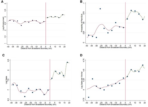
(a) Plant employment. (b) Plant exit propensity. (c) Firm sales. (d) Firm labor productivity.
Notes: The performance variables in Figure 5 (a–d) include plant employment in logs, the plant exit propensity (a plant alive in the business register in year t−1 being dead in year t), log firm sales and log firm sales per worker as a proxy for labor productivity (few firms report value added). Distance from broadband boundary is measured in kilometers. The location of the boundary is determined by the postcode boundary of the telephone exchange area of broadband enable exchanges, up to a maximum distance (5.5 km) that firms could receive an ADSL broadband connection. Positive values of distance are given to plants in locations where broadband is available and negative values to plants in locations where it is not. Observations are grouped into 4 km bins and the data points in the figure represent the average value of observations within that bin. We also report the local polynomial regression lines using observations for different sides of the boundary.
6. Regression results
6.1. OLS estimation
To provide a comparison with the existing literature, we begin by reporting simple conditional correlations between the use of broadband and firm/plant performance metrics. In Table 1, we present simple OLS regressions that show the correlation between broadband adoption and the size of the plant, as measured by the log of employment. To ensure comparability with the results using fuzzy regression-discontinuity estimators, we estimate these OLS regressions for the same set of observations we use in later sections of the paper. We find those that have adopted broadband are typically larger than those that have not (see regression 1), confirming the positive relationship found between employment and broadband use by Haller and Lyons (2015). We find that users of broadband are on average 70% larger than nonusers when we add a parsimonious set controls for age, foreign ownership and multi-plant status (Column 1).31 This figure increases to 114% when we also add year dummies (regression 2). This would appear to suggest that common year-specific shocks are an important presence in the data. Most firms in our regression sample are only observed once and excluding firms for whom geographic discontinuities in broadband infrastructure access persist across multiple years does not affect the results substantially (regression 3). Similarly, adding more restrictive fixed effects (FEs), including industry–year, as well as region dummies, does not substantially change the correlations beyond the inclusion of year dummies alone (regression 4)—with broadband being correlated with around 100% higher employment.32
OLS Correlations of plant employment and broadband use
| Dependent variable: | Plant employment | |||||||
|---|---|---|---|---|---|---|---|---|
| (1) | (2) | (3) | (4) | (5) | (6) | (7) | (8) | |
| — | — | — | — | |||||
| Broadband | 0.530*** | 0.762*** | 0.714*** | 0.695*** | — | — | — | — |
| (0.034) | (0.039) | (0.040) | (0.035) | — | — | — | — | |
| Broadband * Rural | — | — | — | — | 0.380*** | 0.638*** | 0.625*** | 0.607*** |
| — | — | — | — | (0.052) | (0.055) | (0.054) | (0.050) | |
| Broadband * Urban | — | — | — | — | 0.544*** | 0.772*** | 0.726*** | 0.708*** |
| — | — | — | — | (0.035) | (0.039) | (0.041) | (0.035) | |
| Year FE | — | √ | √ | — | — | √ | √ | — |
| Industry–Year FE | — | — | — | √ | — | — | — | √ |
| Region FE | — | — | — | √ | — | — | — | √ |
| Excluding panel obs. | — | — | √ | — | — | — | √ | — |
| Test Urban = Rural (t-stat) | — | — | — | — | 3.579*** | 2.954*** | 2.272** | 2.385** |
| Observations | 36,487 | 36,487 | 22,450 | 36,132 | 36,257 | 36,257 | 22,317 | 36,132 |
Notes: The table presents plant level regressions of broadband use on (log) employment. Excluding panel observations examines robustness to restricting the sample to plants only observed once in our regression sample. Data period 2000–2004. All regressions include control variables for firm age, foreign ownership and a multi-plant dummy, these coefficients are not reported for the sake of parsimony. All regressions include plants in both urban and rural locations across the UK. The variable ‘Broadband * Rural’ is defined as Broadband multiplied by a rural location dummy, similarly ‘Broadband * Urban’ is Broadband multiplied by an urban location dummy. Industries are measured at the three-digit SIC level and regions refer to government office regions. ***, ** and * indicate significance at the 1, 5 and 10% level, respectively, with standard errors clustered at the firm-level reported in parentheses.
In regressions 5–8, we allow the effects of broadband to differ between firms in urban and rural locations. Broadband users are on average 46% larger in rural areas and 72% larger in urban areas in regression 5. When we add the year dummies in Column 6 these effects increase to 90% and 115% respectively, and these correlations are largely unchanged by focusing on firms observed only once or adding various industry, year or region FEs (Columns 7 and 8). In the second from last row of the table, we report the result of a t-test for the null hypothesis that the effects of broadband in urban and rural locations are equal. In both cases, we reject the null and conclude that the effects of broadband are statistically significantly different for firms in these locations. That the effects of the internet are positive but smaller for firms in rural locations than urban areas is consistent with evidence from the existing literature (Fabritz, 2013; Younjun and Orazen, 2017).
We report the correlations between other plant and firm outcomes and broadband use in Appendix Table A2. We find adopting broadband is significantly positively correlated with the level and growth of firm sales and labor productivity (sales per employee), and significantly negatively correlated with plant exit rates. This also holds when we separate urban and rural firms. The evidence for a correlation with employment growth is weaker—we find a weak correlation with broadband amongst urban firms only. In general, the estimated coefficients follow the same pattern as employment and are larger for urban firms, with the exception of sales growth.
6.2. FRD estimation
Next, we present below our FRD results for plant-level employment, before considering urban and rural firms separately.33 For all our outcome variables, the polynomial that minimizes the Akaike Information Criterion is found to be either a linear (regressions 1 and 3) or a linear interaction model (regressions 2 and 4).34 Accordingly, we report both specifications and omit the results of higher order quadratic and cubic polynomials for brevity. In regressions 1 and 2 of the table, we again include firm age, multi-plant status and foreign ownership as controls and in regressions 3 and 4, we add year dummies to control for common shocks.
Pooling across all locations, we find strong evidence of a discontinuity in broadband adoption by plants at the boundary of ADSL-enabled telephone exchanges, as suggested by the earlier evidence in Figure 1a. In Table 2, the first-stage results show that being inside the ADSL-enabled boundary (denoted by the ‘ADSL Boundary’ variable) increases broadband adoption propensity by between 15% and 28% (see regressions 1–8) depending on the control variables added. The Cragg–Donald F-statistic suggests that this variable is a very strong predictor of broadband adoption, easily exceeding the Douglas and Stock (1997) critical values for strong instruments.
Fuzzy regression discontinuity estimates of the effects of broadband use on plant employment—all locations
| Dependent variable: | Plant employment | |||||||
|---|---|---|---|---|---|---|---|---|
| (1) | (2) | (3) | (4) | (5) | (6) | (7) | (8) | |
| Linear | Linear interaction | Linear | Linear interaction | Linear | Linear interaction | Linear | Linear interaction | |
| Second Stage: | ||||||||
| Broadband | 0.249 | 0.235 | 1.046*** | 1.031*** | 1.004*** | 0.979*** | 0.733*** | 0.727*** |
| (0.157) | (0.151) | (0.240) | (0.235) | (0.252) | (0.247) | (0.242) | (0.238) | |
| First Stage—Broadband: | ||||||||
| Boundary | 0.274*** | 0.283*** | 0.175*** | 0.178*** | 0.177*** | 0.180*** | 0.154*** | 0.156*** |
| (0.013) | (0.013) | (0.014) | (0.013) | (0.014) | (0.014) | (0.012) | (0.011) | |
| Year FE | — | — | √ | √ | √ | √ | — | — |
| Industry–Year FE | — | — | — | — | — | — | √ | √ |
| Region FE | — | — | — | — | — | — | √ | √ |
| Excluding panel obs. | — | — | — | — | √ | √ | — | — |
| Cragg–Donald F-Statistic | 915.33 | 978.17 | 399.73 | 411.80 | 276.55 | 284.22 | 317.88 | 322.83 |
| Kleibergen–Papp F-Statistic | 421.08 | 467.87 | 166.73 | 174.16 | 167.93 | 177.05 | 178.65 | 184.99 |
| Akaike Information Criterion | 134,350 | 134,376 | 133,354 | 133,331 | 79,856 | 79,829 | 126,579 | 80,826 |
| Observations | 36,487 | 36,487 | 36,487 | 36,487 | 22,450 | 22,450 | 36,132 | 36,132 |
Notes: The table presents parametric regression discontinuity estimates of the treatment effect of broadband use on plant (the log) of plant employment. Excluding panel, observations examine robustness to restricting the sample to plants only observed once in our data. Data period 2000–2004. We choose not to report the coefficient estimates for the polynomial functions and the other control variables (firm age, foreign ownership and a multi-plant dummy) for the sake of parsimony. The polynomial function is chosen according to the specification that minimizes the Akaike Information Criterion. The first-stage results refer to the effect of being attached to an ADSL broadband-enabled telephone exchange on the likelihood of a plant using broadband. All regressions include plants in both urban and rural locations across the UK. Industries are measured at the three-digit SIC level and regions refer to government office regions. ***, ** and * indicate significance at the 1, 5 and 10% level, respectively, with standard errors clustered at the firm-level reported in parentheses.
In the second stage, we find for the pooled urban and rural data that broadband adoption causes increases in employment.35 In this regard, we are able to confirm findings elsewhere in the literature that also found strong effects for ICT in rural locations including by Fabritz (2013), Younjun and Orazen (2017) and Canzian et al. (2019). According to the results in regression 1, adopting broadband because of being just inside the ADSL-enabled area does not lead to a statistically significant increase in employment (over the period 2000–2004). However, we find larger, positive employment effects when we control for common shocks using year dummies in regression 3 at 185%.
Our regression sample is largely cross-sectional and most plants (22,450 plants) therefore only appear in 1 year. We explore whether the inclusion of persistent differences in broadband access explain our findings in Columns 5 and 6 of Table 2, by excluding plants from the regression sample that are observed for more than one time period. This has no effect on the results compared to the remaining regressions in Table 2, suggesting the inclusion of the same plants at multiple points in time does not explain our main findings.
Finally, we include more restrictive (three-digit SIC) industry–year and region FEs in Columns 7 and 8, our preferred specification. These dummies control for time invariant regional differences, and also capture all industry changes over time that are common across firms. Including these additional FEs does not substantially affect our results, in our sample broadband leads to around 108% higher employment (over 2000–2004). Note the estimated coefficients are of a broadly similar magnitude to the earlier OLS estimates (see Table 1, Column 4).
In Table 3, we compare the effects of broadband on firms in urban and rural locations separately, a main contribution of this article. As reported in Appendix Table A3 the ADSL broadband boundary is a strong predictor of firm broadband adoption in both urban and rural locations, indicated by the size of the first-stage F-statistics, and consistent with earlier discontinuity graphs (Figure 1b and c). The second-stage results in Table 3 reveal some sensitivity of the results for rural firms to the inclusion of different control variables, namely year dummies. In Columns 1 and 2, where we control for age, foreign ownership and multi-plant status only, the effects of broadband on firm performance are apparent only for firms in urban areas. For rural firms, the effect of broadband on employment is statistically insignificant at conventional levels in Columns 1 and 2. This result appears to be driven by a failure to account for year-specific shocks. Once these are controlled for in Columns 3 and 4, we now find strong significant effects on employment amongst plants induced to adopt broadband because of the instrument. These results are consistent whether the distance polynomial is linear or a linear interaction. Moreover, this pattern of results continues to hold when we use plants separated by differences in access to broadband for only a single year (regressions 5 and 6). The pattern also persists by including industry–year and region FEs (regressions 7 and 8), our preferred specification.
Fuzzy regression discontinuity estimates of the effects of broadband use on plant employment—rural versus urban locations
| Dependent variable: | Plant employment | |||||||
|---|---|---|---|---|---|---|---|---|
| (1) | (2) | (3) | (4) | (5) | (6) | (7) | (8) | |
| Linear | Linear interaction | Linear | Linear interaction | Linear | Linear interaction | Linear | Linear Interaction | |
| Second Stage: | ||||||||
| Broadband * Rural | −0.170 | −0.191 | 0.802*** | 0.773*** | 0.814*** | 0.773*** | 0.490* | 0.476* |
| (0.158) | (0.152) | (0.271) | (0.265) | (0.274) | (0.268) | (0.265) | (0.261) | |
| Broadband * Urban | 0.232 | 0.216 | 1.007*** | 0.986*** | 0.991*** | 0.961*** | 0.706*** | 0.694*** |
| (0.159) | (0.153) | (0.243) | (0.239) | (0.251) | (0.247) | (0.244) | (0.241) | |
| Year FE | — | — | √ | √ | √ | √ | — | — |
| Industry–Year FE | — | — | — | — | — | — | √ | √ |
| Region FE | — | — | — | — | — | — | √ | √ |
| Excluding panel obs. | — | — | — | — | √ | √ | — | — |
| Cragg–Donald F-Statistic | 464.25 | 496.96 | 189.10 | 194.18 | 135.77 | 139.17 | 152.70 | 154.49 |
| Kleibergen–Papp F-Statistic | 215.27 | 240.90 | 74.94 | 78.28 | 79.72 | 83.91 | 82.92 | 85.57 |
| Akaike Information Criterion | 133,685 | 133,723 | 132,450 | 132,423 | 79,374 | 79,345 | 126,582 | 126,585 |
| Test Urban = Rural (t-stat) | 7.081*** | 7.106*** | 3.454*** | 3.625*** | 3.089*** | 3.299*** | 4.023*** | 4.051*** |
| Observations | 36,257 | 36,257 | 36,257 | 36,257 | 22,317 | 22,317 | 36,132 | 36,132 |
Notes: The table presents parametric regression discontinuity estimates of the treatment effect of broadband use on plant (the log) of plant employment. Excluding panel observations examines robustness to restricting the sample to plants only observed once in our data. Data period 2000–2004. We choose not to report the coefficient estimates for the polynomial functions and the other control variables (firm age, foreign ownership and a multi-plant dummy) for the sake of parsimony. The polynomial function is chosen according to the specification that minimizes the Akaike Information Criterion. Two treatment effects are estimated, interacting Broadband adoption with a rural dummy and an urban dummy. The first-stage results refer to the effect of being attached to an ADSL broadband-enabled telephone exchange on the likelihood of a plant using broadband. Industries are measured at the three-digit SIC level and regions refer to government office regions. The first-stage results are omitted for brevity and reported in Appendix Table A3. ***, ** and * indicate significance at the 1, 5 and 10% level, respectively, with standard errors clustered at the firm-level reported in parentheses.
The effect of broadband is positive but smaller in rural compared to urban regions, at 61% and 100%, respectively (see regression 8). This difference is confirmed by the statistical test of the hypothesis that they are equal (the results of this t-test are reported toward the bottom of the table). Comparing across the results leads us to conclude there is evidence of a causal effect of access to low-cost broadband on plant employment for urban and rural firms once we use a methodology that randomizes difficult to observe confounding factors such as managerial ability across treatment and control groups and once we control for common shocks to the economy.
We examine the robustness of these results to the inclusion of region–year and industry effects, to allow differences in shocks across NUTS-2-level regions reported in Appendix Table A5. They also continue to hold when we add both region–year and industry–year FEs in Appendix Appendix Table A6, out of a concern that unobserved industry or region differences may be adding noise to our estimations. If potentially confounding factors are randomly distributed along the geographic broadband discontinuity, then additional controls are not needed, but they can improve precision. We find that the identification remains largely unchanged compared to Tables 2 and 3, with similarly sized F-statistics and ADSL broadband availability leading to around a 15% increase in broadband adoption. With these additional FEs, in the second stage, we find that broadband leads to somewhat larger increases in employment than the baseline in Table 2. An increase in the employment of urban plants of around 150% in regression 4 in Appendix Table A5 and 116% in Appendix Table A6 (compared to 100% for the same regression in Table 2) and an increase in rural plant employment of around 108% in Appendix Table A5 and 76% in Appendix Table A6 (compared to 61% in Table 2).
In Table 4, we explore the effects of broadband on a range of other outcome variables. In regressions 1 and 2, we report the effect on plant exit. Information on sales is available only at the level of the firm within the ONS data, and we report the results for this variable in regressions 3 and 4. In regressions 5 and 6, we consider the effects on labor productivity, measured as sales per employee. The first stage of these regressions is reported in Appendix Table A8 for brevity. The results in regression 1 suggest no strong effect on the exit of plants. For sales, we find strong and statistically significant positive effects of broadband adoption on the sales of firms in urban areas, whereas for rural areas the point estimates are both smaller and not significantly different from zero. This difference is again confirmed from a t-test that the coefficients for urban and rural firms are equal reported toward the bottom of the table. For labor productivity, we find no significant effects, indicating that the sales and employment effects are broadly balanced. The absence of any effect on labor productivity in our results contrasts with a number of the studies reviewed by Cardona et al. (2013) or Bertschek et al. (2015) and would appear to suggest that significant effects found previously, including when using OLS estimators, are explained by the presence of unobservable confounders. Our results are consistent with DeStefano et al. (2018), who use a different identification strategy for firms in urban locations and find that broadband leads to an increase in firm scale, but not labor productivity or total factor productivity.
Fuzzy regression discontinuity estimates of the effects of broadband use on firm performance—rural versus urban locations
| Dependent variable: | Plant exit | Firm sales | Firm labor productivity | |||
|---|---|---|---|---|---|---|
| (1) | (2) | (3) | (4) | (5) | (6) | |
| Linear | Linear interaction | Linear | Linear interaction | Linear | Linear interaction | |
| Second Stage: | ||||||
| Broadband * Rural | −0.000 | 0.008 | 0.590 | 0.587 | 0.062 | 0.060 |
| (0.036) | (0.036) | (0.407) | (0.407) | (0.243) | (0.242) | |
| Broadband * Urban | 0.002 | 0.009 | 1.192*** | 1.204*** | 0.219 | 0.224 |
| (0.033) | (0.032) | (0.347) | (0.348) | (0.207) | (0.207) | |
| Industry–Year FE | √ | √ | √ | √ | √ | √ |
| Region FE | √ | √ | √ | √ | √ | √ |
| Cragg–Donald F-statistic | 148.82 | 150.32 | 76.21 | 75.89 | 76.21 | 75.89 |
| Kleibergen–Papp F-Statistic | 90.62 | 93.20 | 74.77 | 74.62 | 74.77 | 74.62 |
| Akaike Information Criterion | −374.18 | −349.67 | 66,284.76 | 66,277.01 | 50,401.61 | 50,396.79 |
| Test: Urban = Rural (t-stat) | 0.274 | 0.109 | 5.281*** | 5.417*** | 2.290** | 2.394** |
| Observations | 32,082 | 32,082 | 17,198 | 17,198 | 17,198 | 17,198 |
Notes: The table presents parametric regression discontinuity estimates of the treatment effect of broadband use on plant and firm-level outcomes. These outcomes include plant exit reflecting the propensity of death at t + 1, (the log) of firm sales and firm labor productivity that reflects sales per worker (value-added is not available for many firms). Data period 2000–2004. We choose not to report the coefficient estimates for the polynomial functions and the other control variables (firm age, foreign ownership and a multi-plant dummy) for the sake of parsimony. The polynomial function is chosen according to the specification that minimizes the Akaike Information Criterion. Two treatment effects are estimated, interacting Broadband adoption with a rural dummy and an urban dummy. The first-stage results refer to the effect of being attached to an ADSL broadband-enabled telephone exchange on the likelihood of a plant using broadband. The first-stage results are omitted for brevity and reported in Appendix Table A8. ***, ** and * indicate significance at the 1, 5 and 10% level, respectively, with standard errors clustered at the firm-level reported in parentheses.
A possibility might be that the effects of improved broadband access reveal themselves more clearly on the growth of employment (Appendix Table A9) or sales (Appendix Table A10). When considering plant employment growth or firm sales growth, the first-stage F-statistics are somewhat weaker than Tables 2 and 3, given fewer observations, but remain above conventional levels for a strong first stage.36 In the second stage, we find no significant effect of rural or urban broadband on employment growth or sales growth.
As a final exercise in this section, we consider the effect of broadband adoption on manufacturing firms. As shown in Appendix Table A11, we have a smaller number of observations in these regressions, but continue to find that the ADSL boundary is a strong predictor of broadband adoption amongst manufacturing firms. Being attached to an ADSL-enabled local telephone exchange increases the probability of adoption by around 12% in Columns 1 and 2. In the second stage, we find some positive effects on employment, but these are less precisely estimated than our baseline of services firms, which might reflect the smaller sample used in these regressions. We find marginally significant evidence for urban firms (at the 10% level), but with slightly smaller coefficients than services firms. For rural manufacturing firms, there are similarly sized point estimates as urban firms, but these have large standard errors so are not statistically different from zero.
6.3. Robustness tests of identifying assumptions
Our regression discontinuity approach relies on firms being unable to precisely sort around the discontinuity. Across the sample, 4124 (around 11%) of observations are of plants that report a different postcode at any point between 1997 and 2008. While it is unlikely that firms move to gain access to broadband given the costs of relocation and the short-term nature of the discontinuities in ADSL broadband access that we study, as a robustness test we rerun the baseline regressions excluding firms that changed postcodes at any time from 1997 to 2007.37 In Appendix Table A12, we repeat our baseline plant employment estimations, now excluding plants that ever move to a different postcode and find the baseline results are unchanged.
We further assess the robustness of our estimates by examining narrow bandwidths in close proximity to the broadband boundary (see Appendix Table A13). A concern that often arises for geographic discontinuities of the type, we use are that there are other discontinuities in our data that we are somehow conflating the results. To assess this, we estimate local linear regressions for a range of bandwidths, from 2.5 to 10 km.38 As shown in Appendix Table A13, the broadband discontinuity strongly predicts firm broadband adoption. In the second stage, the findings are somewhat weaker than the baseline estimates, with positive effects of broadband on employment for firms overall and for firms in urban areas in most specifications. For rural firms, the estimates are more imprecisely estimated, with relatively large standard errors, meaning the point estimates are not significantly different from zero.
7. Heterogeneity
Previous evidence from Bloom et al. (2014), DeStefano et al. (2020) and others have shown heterogeneity in the effects of ICT across industries. In this section, we use this evidence to motivate an exploration of heterogeneity in the effects of broadband across according to the knowledge intensity of the sector. We use three alternative measures. The first is an Organisation for Economic Co-operation and Development (OECD) indicator detailed in McNicoll et al. (2002) and which we label high knowledge sector (HKS) which takes into account expenditures in R&D toward technology development, the degree to which technology is being used and the overall skill of the workforce based on average occupational activities at the two-digit sector level. The second indicator is calculated using Eurostat (2014) and is defined as sectors where over a third of employees have tertiary level education labeled at Knowledge Intensive Activity (KIA) sectors. Finally, we use a measure of knowledge intensity based on R&D, where we define knowledge-intensive sectors as those in the top quartile of R&D expenditure using ONS data on R&D expenditures consistent with Galindo-Rueda and Verger (2016). In each case we allow the effects of these knowledge-intensive sectors to differ between firms in urban and rural locations. The dummy variables are specified such that the rural or urban dummy captures the effect of broadband in firms in low KIA/HKS sectors and the interaction between urban/rural and these KIA/HKS sectors is being measured relative to that. The results from this exercise are presented in Table 5.
Industry heterogeneity
| Dependent variable: | Plant employment | |||||
|---|---|---|---|---|---|---|
| (1) | (2) | (3) | (4) | (5) | (6) | |
| Linear | Linear interaction | Linear | Linear interaction | Linear | Linear interaction | |
| Second Stage: | ||||||
| Broadband * Rural | 0.141 | 0.132 | 0.192 | 0.185 | 0.388 | 0.372 |
| (0.306) | (0.301) | (0.300) | (0.295) | (0.271) | (0.267) | |
| Broadband * Rural* KIA | 0.857** | 0.861** | — | — | — | — |
| (0.361) | (0.360) | — | — | — | — | |
| Broadband * Rural* HKS | — | — | 0.811** | 0.812** | — | — |
| — | — | (0.359) | (0.358) | — | — | |
| Broadband * Rural* R&D | — | — | — | — | 1.166* | 1.174* |
| — | — | — | — | (0.669) | (0.669) | |
| Broadband * Urban | 0.271 | 0.264 | 0.322 | 0.316 | 0.602** | 0.589** |
| (0.287) | (0.282) | (0.278) | (0.274) | (0.250) | (0.247) | |
| Broadband * Urban * KIA | 1.145*** | 1.148*** | — | — | — | — |
| (0.298) | (0.297) | — | — | — | — | |
| Broadband * Urban * HKS | — | — | 1.158*** | 1.159*** | — | — |
| — | — | (0.298) | (0.298) | — | — | |
| Broadband * Urban * R&D | — | — | — | — | 1.172** | 1.179** |
| — | — | — | — | (0.537) | (0.536) | |
| Industry–Year FE | √ | √ | √ | √ | √ | √ |
| Region FE | √ | √ | √ | √ | √ | √ |
| Cragg–Donald F-statistic | 72.39 | 73.58 | 74.81 | 75.87 | 76.03 | 76.92 |
| Kleibergen–Papp F-Statistic | 34.74 | 36.22 | 38.11 | 39.61 | 41.46 | 42.81 |
| Akaike Information Criterion | 127,105 | 127,114 | 127,095 | 127,101 | 126,651 | 126,659 |
| Observations | 36,132 | 36,132 | 36,132 | 36,132 | 36,132 | 36,132 |
Notes: The table presents parametric regression discontinuity estimates of the treatment effect of broadband use on plant and firm-level outcomes. These outcomes include (the log) of plant employment. KIA refers to knowledge-intensive sectors, those where at least 33% of the workforce have a tertiary education as defined by Eurostat (2014). R&D intensity is calculated by taking the ratio of R&D expenditure over gross value added at the two-digit sector level similar to consistent to Galindo-Rueda and Verger (2016). Firms are then classified as being in R&D intensive if their sector is in the top quartile of R&D intensity. HKS is a composite measure which takes into account expenditures in R&D toward technology development, the degree to which technology is being used and the overall skill of the workforce based on average occupational activities at the two-digit sector level (McNicoll et al., 2002). Data period 2000–2004. We choose not to report the coefficient estimates for the polynomial functions and the other control variables (firm age, foreign ownership and a multi-plant dummy) for the sake of parsimony. Industries are measured at the three-digit SIC level and regions refer to government office regions. The polynomial function is chosen according to the specification that minimizes the Akaike Information Criterion. Two treatment effects are estimated, interacting Broadband adoption with a rural dummy and an urban dummy. The first-stage results refer to the effect of being attached to an ADSL broadband-enabled telephone exchange on the likelihood of a plant using broadband. The first-stage results are omitted for brevity. ***, ** and * indicate significance at the 1, 5 and 10% level, respectively, with standard errors clustered at the firm level reported in parentheses.
We find strong evidence of heterogeneity across industries with the positive employment effects of broadband concentrated within a subset of sectors. For rural firms, we find broadband in low KIA, low HKS or low R&D intensity sectors has effects that are much smaller than the earlier estimates we derived across all sectors and that these are not significantly different from zero (see the coefficients on Broadband*Rural in Table 5). In contrast, rural firms in high KIA sectors have 137% higher employment effects of broadband than those in low KIA sectors and similarly rural firms in high HKS or high R&D intensive sectors have 125% and 224%, respectively, greater employment effects than their low-intensity counterparts. This suggests the earlier effects for rural firms observed earlier are concentrated in firms operating in knowledge and R&D intensive sectors.
For urban firms, we also find no employment effects of broadband in low-KIA or low-HKS sectors, but broadband adoption leads to 80% increase in employment in less R&D-intensive sectors. Similarly, the employment effects of broadband are much larger for urban firms in high KIA, HKS or R&D sectors. Urban firms engaged in KIA sectors have 214% higher employment effects of broadband than those less knowledge intensive. Of note is that the effects of urban firms in high knowledge-intensive sectors appear to be larger than rural firms operating in these same sectors.39 This would appear to suggest agglomeration factors such as knowledge spillovers or well-developed input and labor markets also play a role in increasing the benefits from broadband adoption amongst urban firms (Combes et al., 2012).
8. Conclusion
This article tests the effects of broadband Internet on firm performance in urban and rural areas. We employ a novel FRD design using geographic discontinuities in broadband availability to elicit causal effects for firms across the whole of the UK. Using this empirical design, we find strong evidence in support of the view that greater access to broadband infrastructure significantly increases the likelihood of adoption in both rural and urban areas. In urban localities, our findings confirm the literature to date, broadband leads to an increase in firm scale (measured by employment or sales) but the link with labor productivity is not statistically significant. We are also able to confirm positive, but smaller effects for rural firms. Given the discontinuity we study likely leads to balance in difficult to observe confounders across treatment and control these results point to an interpretation of causal effects. It, therefore, seems that universal broadband policies may lead to substantial economic benefits to firms in rural areas. However, these effects are not universal, but they are concentrated in firms operating in knowledge-intensive sectors. These benefits likely depend on the local industry composition, especially the ability to benefit from knowledge-intensive activities, and may not materialize for rural firms universally.
Our results provide support to the expectations underlying universal broadband policies. Both domestic policy makers and international agencies have supported policies aimed firstly at improving access to and secondly the speed of internet connections across countries with a view to increasing both employment and productivity. Direct policy interventions have included actions to stimulate demand as well as those to affect the supply side, such as obligations for universal service and subsides for infrastructure provision. For example, in the last decade, the European Commission launched a number of initiatives including eEurope, eEurope2005 and i2010 (Falch, 2007); while US action was provided through the Federal Rural Broadband Access Loans and the Community Connect Broadband Grant programs as well as other initiatives at the state and local government level. In 2010, the UK Government announced a target of universal access to basic broadband by 2013, super-fast broadband by 2015 and for the UK to have the fastest network speeds of the five largest EU economies. It has committed £1.7 billion of public funds to support private investment in broadband infrastructure between 2013 and 2017 (Department for Culture Media and Sport, 2013b). The UK Culture Secretary (Jeremy Hunt) explained the motivation behind this as ‘(T)he reason we want to do this is very simple—it is about jobs’. Whilst this article cannot comment on the effect of advances in speeds due to super-fast broadband, our results indicate that this view has empirical support.
Funding
Harvard Business School, Division of Research and Faculty Development provided funds for the research.
Footnotes
This work contains statistical data from the Office for National Statistics (ONS) and supplied by the Secure Data Service at the UK Data Archive. The data are Crown Copyright and reproduced with the permission of the controller of HMSO and Queen s Printer for Scotland. The use of the data in this work does not imply the endorsement of ONS or the Secure Data Service at the UK Data Archive in relation to the interpretation or analysis of the data. This work uses research datasets, which may not exactly reproduce National Statistics aggregates.
For example, 62% of the EU has access to 30 Mbps broadband, whereas in rural areas only 18% do so (European Commission, 2014).
Our data allow us to measure some outcomes, such as employment, at the level of the plant and others, such as sales, as the more aggregated level of the firm. We focus our analysis on employment. We abstract from this point in the introduction and use the more familiar term of firms for ease.
See for example, Van Gaasbeck (2008), Grimes et al. (2012), Kolko (2012), Bertschek et al. (2013), Akerman et al. (2015), and Haller and Lyons (2015).
In this regard, our empirical design is closest to Falck et al. (2014) who study the effect of differences in internet access on voting behavior in Germany and, written concurrent with this paper, Faber et al. (2016) who study broadband access on educational attainment, and Ahlfeldt et al. (2017) who study the effect on property prices, both for the UK.
In the next section of the paper, we provide more detail on the location of the discontinuities that we exploit.
It is also worthy to note that the spatial discontinuity exists for the availability of broadband but no other technologies, in particular mobile technologies, that developed around this time.
In Figure 1, firms in non-enabled areas have non-zero broadband take-up due to the availability of leased line and cable broadband prior to the start of our sample, which is particularly the case in urban areas.
See Lee and Lemieux (2010) for a review of the literature on regression discontinuity designs.
Akerman et al. (2015) report that Norwegian firms that start to use broadband increase their use of skilled labor and Bloom et al. (2014) which explore the effects of intranets on the level of decision making cross-European data. In both cases these effects are short-run, occurring within a three-year window. Evidence of other firm level impacts in a variety of country contexts can be found in Van Gaasbeck (2008), Grimes et al. (2012), Kolko (2012), Bertschek et al. (2013) and Haller and Lyons (2015).
To our knowledge, only one broadband delivery program explicitly targeting rural areas has been evaluated to date (the US Rural Broadband Loan Program), providing mixed results with positive effects on local employment, wages and firm entry (Kandilov and Renkow, 2010; Younjun and Orazem, 2017). Based on propensity score matching strategies, Whitacre et al. (2014) find that higher levels of broadband adoption in US rural areas led to increased income growth and unemployment reduction.
The asymmetry refers to greater bandwidth allocated downstream than upstream, meaning faster download speeds at the expense of slower uploading of data.
In urban areas in the UK, high-speed fibre-broadband was rolled out from 2009 until 2014.
Telephone services could be delivered up to 16 km. The signal for voice calls is boosted by so-called loading coils, meaning that the quality of telephone signals could potentially be maintained for up to 16 km from the exchange (Macassey, 1985). Loading coils are not compatible with ADSL.
Cable broadband packages available were also a little more costly than ADSL, at £15–£35 per month for a 2–10 Mbits/second cable connection, compared to £12–£17 per month an average 1 Mbits/second ADSL connection (Downes, 2007).
The exception to this is in the North East of England where, as a result of a historical accident, a small number of exchanges are operated by a separate telecoms provider. The working version of this paper used this region as a robustness test. The results suggest that the effects of broadband are statistically insignificant, but with a large standard error such that they are poorly identified zero effects. For this reason we have not included these results in the paper.
The enablement of ADSL required that the local exchange be equipped with DSL capability and the end-user premises were fitted with a modem and micro-filter device (ADSL splitter). The ability of other providers to install their own ADSL equipment, known as Local Loop Unbundling, was negligible until at least 2005, when fewer than 2% of telephone lines were ‘unbundled’ for other providers to offer services (Cadman, 2012).
BT had been trialing ADSL since 1994 and analysis at the time suggests that BT delayed rolling out ADSL in order to protect its national monopoly on existing narrowband technologies, such as ISDN (BBC News, 1999).
Within the regression sample of 36,487 some 3384 observations are for the year 2000. This increases to 4614 and 4701 in 2001 and 2002, increasing again in 2003 to 9234 and 15,123 in 2004.
Figures for the city of London are reported within Faber et al. (2016), who follow the same approach as this paper.
See Griffith (1999) for a description of the data, the data references are noted at the end of the paper.
Note that this is likely because any labor productivity effect encompasses both improvements in TFP as well as capital deepening (Cardona et al., 2013).
Given the change in the sampling frame after the initial survey in 2000, we have tested the effect of excluding the observations from this year. The results from this are reported in Table A7 and are consistent with the baseline.
We find the very similar results using data from PointTopic, which for a subset of UK postcodes details the telephone exchange each postcode is connected to (see DeStefano et al., 2018). A similar exercise, for the North-East of the UK shows the crow-flies mapping is a good proxy and encompasses all of the zip codes OFCOM identifies as being served by KC.
We do not include time subscripts on observations to reflect the fact that the location of the discontinuity in broadband access changes across time. Neighboring plants/firms only appear in the regression sample when they are separated by a discontinuity in broadband access. We return to this point in Section 6.
An alternative mechanism of specification selection in sharp discontinuity designs is to employ an F-test method (Lee and Lemieux, 2010), however, this is not appropriate for a fuzzy design, since two-stage least squares estimation R-squared are not informative (Wooldridge, 2010).
Results are available upon request.
We group the observations into 4 km bins, which is suggested by both the F-test and bin dummy methods of Lee and Lemieux (2010).
Graphs of the key outcome variables against distance to the ADSL for urban and rural firms are consistent with the empirical results. The figures are excluded for brevity and are available upon request.
Appendix Figure A1(A and B) graphs sales growth and employment growth against distance to the ADSL boundary. These show evidence of a discontinuity for sales growth, but not employment growth.
While there is some noise on both sides of the threshold (which is common amongst RDDs), say 20 km from the boundary, importantly the discontinuity present in Figure 5(A–C) and absent in 5D is precisely around the threshold.
Since the regression is log-linear, 70% is calculated as exp(0.530)−1, using the estimated coefficient from Column 1.
Note we later consider robustness to including even more restrictive fixed effects.
A linear interaction model is a linear model with a change in slope at the discontinuity.
This result also holds for rural firms when we estimate them separately (Table A4). For urban firms estimated alone we do not find any second stage effects, likely because the identification is weaker than when estimating only rural firms or in the pooled sample.
The sample size is lower in terms of growth rather than level variables, since it requires a balanced panel of observations.
Note that this also controls for any relocation by firms 3 years before that start of the ADSL rollout period, thereby eliminating anticipation effects.
We estimated both local linear regressions with and without slope changes at the boundary, but report those without slope changes since these minimize the Akaike Information Criterion for each bandwidth.
The differential between R&D intensive and less-intensive sectors is similar in urban and rural firms, however, urban firms in less-R&D intensive sectors have positive effects of broadband.
References
Data references
Appendix: Additional Results and Summary Statistics

(a) Plant employment growth. (b) Firm sales growth.
Notes: The performance variables in Figures B1 (a and b) reflect (1-year) growth in plant employment and growth in firm sales. Distance from broadband boundary is measured in kilometers. The location of the boundary is determined by the postcode boundary of the telephone exchange area of broadband enable exchanges, up to a maximum distance (5.5 km) that firms could receive an ADSL broadband connection. Positive values of distance are given to plants in locations where broadband is available and negative values to plants in locations where it is not. Observations are grouped into 4 km bins and the data points in the figure represent the average value of observations within that bin. We also report the local polynomial regression lines using observations for different sides of the boundary.
Summary statistics—baseline sample
| Variables | All firms | Urban | Rural | ||||||
|---|---|---|---|---|---|---|---|---|---|
| Observations | Mean | Standard Deviation | Observations | Mean | Standard Deviation | Observations | Mean | Standard Deviation | |
| Plant employment | 37,291 | 63.022 | 134.886 | 31,106 | 66.43095 | 139.7915 | 5950 | 45.54857 | 105.1176 |
| Plant employment growth | 10,537 | 0.004 | 0.412 | 9054 | 0.005 | 0.423 | 1392 | −0.004 | 0.352 |
| Plant exit | 32,452 | 0.065 | 0.247 | 26,995 | 0.068 | 0.252 | 5250 | 0.050 | 0.217 |
| Broadband use | 37,291 | 0.591 | 0.492 | 31,106 | 0.623 | 0.485 | 5950 | 0.429 | 0.495 |
| Urban plant | 37,056 | 0.839 | 0.367 | 31,106 | 1.000 | 0.000 | 5950 | 0.000 | 0.000 |
| Plant moves postcode units (1997–2008) | 37,291 | 0.061 | 0.239 | 31,106 | 0.112 | 0.315 | 5950 | 0.104 | 0.306 |
| Firm sales | 18,274 | 54,742.69 | 1,173,357 | 14,535 | 65,355.8 | 1,313,788 | 3644 | 13,374.95 | 131,696.8 |
| Firm sales growth | 3500 | 0.061 | 0.602 | 2884 | 0.058 | 0.621 | 594 | 0.079 | 0.507 |
| Firm sales per worker | 18,274 | 291.670 | 4608.036 | 14,535 | 327.446 | 5159.146 | 3644 | 151.566 | 539.131 |
| Firm age | 17,505 | 14.674 | 9.702 | 13,942 | 14.808 | 9.699 | 3473 | 14.111 | 9.698 |
| Firm is multi-plant | 18,275 | 0.244 | 0.429 | 14,535 | 0.266 | 0.442 | 3645 | 0.155 | 0.362 |
| Firm is foreign owned | 18,275 | 0.097 | 0.296 | 14,535 | 0.108 | 0.310 | 3645 | 0.054 | 0.226 |
| Knowledge-intensive sector | 37,291 | 0.329 | 0.470 | 37,291 | 0.329 | 0.470 | 5950 | 0.272 | 0.445 |
| Human capital intensive sector | 37,291 | 0.290 | 0.454 | 37,291 | 0.290 | 0.454 | 5950 | 0.237 | 0.425 |
| R&D-intensive sector | 37,291 | 0.060 | 0.237 | 37,291 | 0.060 | 0.237 | 5950 | 0.068 | 0.252 |
Notes: Sales and Sales per Worker are in 1000s of pound sterling (2005 prices deflated using two-digit industry PPI), Employment reflects the plant employee headcount and Plant Exit that reflects the propensity of death at t + 1. Firm Age is measured in years. Broadband use is a zero-one indicator of whether the firm uses (recorded as a 1) broadband or not (recorded as a zero). All growth variables refer to a 1-year difference in logs. Employment, broadband use, industry and plant exit refer to plant-level observations. Sales, age, multi-plant, age and foreign ownership refer to firm-level observations. Knowledge-intensive sector refers to those where at least 33% of the workforce has a tertiary education as defined by Eurostat (2014). R&D intensity is calculated by taking the ratio of R&D expenditure over gross value added at the two-digit sector level similar to consistent to Galindo-Rueda and Verger (2016). Firms are then classified as being in R&D intensive if their sector is in the top quartile of R&D intensity. Human Capital Intensive Sector is a composite measure which takes into account expenditures in R&D toward technology development, the degree to which technology is being used and the overall skill of the workforce based on average occupational activities at the two-digit sector level (McNicoll et al., 2002).
OLS Regressions of plant and firm outcomes and broadband use
| Dependent variable: | Plant exit | Firm sales | Firm labor productivity | Plant employment | Firm Sales | |||||
|---|---|---|---|---|---|---|---|---|---|---|
| Growth | Growth | |||||||||
| (1) | (2) | (3) | (4) | (5) | (6) | (7) | (8) | (9) | (10) | |
| Broadband | −0.019*** | 1.297*** | 0.299*** | 0.026* | 0.068*** | |||||
| (0.005) | (0.035) | (0.022) | (0.014) | (0.022) | ||||||
| Broadband * Rural | — | −0.017** | — | 1.046*** | — | 0.180*** | — | 0.015 | 0.119*** | |
| — | (0.007) | — | (0.069) | — | (0.043) | — | (0.020) | (0.039) | ||
| Broadband * Urban | — | −0.019*** | — | 1.338*** | — | 0.319*** | — | 0.027* | 0.059*** | |
| — | (0.006) | — | (0.037) | — | (0.022) | — | (0.015) | (0.022) | ||
| Industry–year FE | √ | √ | √ | √ | √ | √ | √ | √ | √ | √ |
| Region FE | √ | √ | √ | √ | √ | √ | √ | √ | √ | √ |
| Test: Urban = Rural (t-stat) | — | 0.320 | — | 4.235*** | — | 3.245*** | — | 0.680 | 1.507 | |
| Observations | 32,082 | 32,082 | 17,198 | 17,198 | 17,198 | 17,198 | 10,348 | 10,348 | 3433 | 3433 |
Notes: The table presents plant-level regressions of broadband use on plant- and firm-level outcomes. These outcomes include plant exit that reflects the propensity of death at t + 1, (the log) of firm sales, firm labor productivity that reflects sales per worker (value-added is not available for many firms), plant employment growth and firm sales growth. All growth variables refer to a 1-year difference in logs. Data period 2000–2004. All regressions include control variables for firm age, foreign ownership and a multi-plant dummy, these coefficients are not reported for the sake of parsimony. All regressions include plants in both urban and rural locations across the UK. Industries are measured at the three-digit SIC level and regions refer to government office regions. ***, ** and * indicate significance at the 1, 5 and 10 level, respectively, with standard errors clustered at the firm-level reported in parentheses.
First stage FRD estimates of the effects of broadband use on plant employment—rural versus urban locations
| Dependent variable: | Plant employment | ||||||||
|---|---|---|---|---|---|---|---|---|---|
| (1) | (2) | (3) | (4) | (5) | (6) | (7) | (8) | ||
| Linear | Linear interaction | Linear | Linear interaction | Linear | Linear interaction | Linear | Linear interaction | ||
| First stage—Broadband * Rural | |||||||||
| Boundary * Rural | 0.554*** | 0.554*** | 0.545*** | 0.544*** | 0.578*** | 0.577*** | 0.543*** | 0.542*** | |
| (0.015) | (0.015) | (0.015) | (0.015) | (0.016) | (0.016) | (0.014) | (0.014) | ||
| Boundary * Urban | −0.104*** | −0.104*** | −0.108*** | −0.108*** | −0.089*** | −0.089*** | −0.105*** | −0.106*** | |
| (0.008) | (0.008) | (0.008) | (0.008) | (0.008) | (0.008) | (0.007) | (0.007) | ||
| First stage—Broadband * Urban | |||||||||
| Boundary * Rural | −0.259*** | −0.246*** | −0.422*** | −0.416*** | −0.437*** | −0.431*** | −0.427*** | −0.424*** | |
| (0.010) | (0.010) | (0.012) | (0.012) | (0.013) | (0.013) | (0.012) | (0.012) | ||
| Boundary * Urban | 0.376*** | 0.384*** | 0.291*** | 0.293*** | 0.272*** | 0.274*** | 0.266*** | 0.268*** | |
| (0.011) | (0.010) | (0.011) | (0.011) | (0.012) | (0.011) | (0.010) | (0.010) | ||
| Year FE | — | — | √ | √ | √ | √ | √ | √ | |
| Industry–year FE | — | — | — | — | — | — | √ | √ | |
| Region FE | — | — | — | — | — | √ | √ | ||
| Excluding panel obs. | — | — | — | — | √ | √ | — | — | |
| Cragg–Donald F-Statistic | 464.25 | 496.96 | 189.10 | 194.18 | 135.77 | 139.17 | 152.70 | 154.49 | |
| Kleibergen–Papp F-Statistic | 215.27 | 240.90 | 74.94 | 78.28 | 79.72 | 83.91 | 82.92 | 85.57 | |
| Akaike Information Criterion | 133,685 | 133,723 | 132,450 | 132,423 | 79,374 | 79,345 | 126,582 | 126,585 | |
| Test Urban = Rural (t-stat) | 7.081*** | 7.106*** | 3.454*** | 3.625*** | 3.089*** | 3.299*** | 4.023*** | 4.051*** | |
| Observations | 36,257 | 36,257 | 36,257 | 36,257 | 22,317 | 22,317 | 36,132 | 36,132 | |
Notes: The table presents the first stage of parametric regression discontinuity estimates of the treatment effect of broadband use on plant (the log) of plant employment—the second stage is reported in Table 3. Excluding panel observations examines robustness to restricting the sample to plants only observed once in our data. Data period 2000–2004. We choose not to report the coefficient estimates for the polynomial functions and the other control variables (firm age, foreign ownership and a multi-plant dummy) for the sake of parsimony. Industries are measured at the three-digit SIC level and regions refer to government office regions. The polynomial function is chosen according to the specification that minimizes the Akaike Information Criterion. The first-stage results refer to the effect of being attached to an ADSL broadband-enabled telephone exchange on the likelihood of a plant using broadband. Broadband boundary is a zero-one indicator equal to one if the plant is inside the area of broadband-enabled telephone exchanges. Two treatment effects are estimated, interacting Broadband adoption with a rural dummy and an urban dummy, and the Boundary instrument is similarly interacted. ***, ** and * indicate significance at the 1, 5 and 10% level, respectively, with standard errors clustered at the firm-level reported in parentheses.
FRD estimates of the effects of broadband use on plant employment—rural and urban locations separately
| Dependent variable: | Plant employment | |||
|---|---|---|---|---|
| (1) | (2) | (3) | (4) | |
| Urban | Rural | |||
| Linear | Linear interaction | Linear | Linear interaction | |
| Second stage: | ||||
| Broadband | 0.736 | 0.685 | 0.735** | 0.754** |
| (0.549) | (0.535) | (0.311) | (0.326) | |
| First stage—Broadband | ||||
| Boundary | 0.105*** | 0.109*** | 0.243*** | 0.237*** |
| (0.017) | (0.017) | (0.022) | (0.022) | |
| Year FE | √ | √ | √ | √ |
| Cragg–Donald F-statistic | 77.41 | 80.40 | 219.68 | 201.10 |
| Kleibergen–Papp F-Statistic | 37.92 | 41.11 | 125.29 | 113.86 |
| Akaike Information Criterion | 114,639.78 | 114,654.52 | 20,939.77 | 20,940.34 |
| Observations | 30,784 | 30,784 | 5798 | 5798 |
Notes: The table presents parametric and nonparametric regression discontinuity estimates of the treatment effect of broadband use on (the log) of employment separating the sample into plants in urban and rural locations. Data period 2000–2004. We choose not to report the coefficient estimates for the polynomial functions and the other control variables (firm age, foreign ownership and a multi-plant dummy) for the sake of parsimony. In the parametric regressions, the polynomial function is chosen according to the specification that minimizes the Akaike Information Criterion. The first-stage results refer to the effect of being attached to an ADSL broadband-enabled telephone exchange on the likelihood of a plant using broadband. Broadband boundary is a zero-one indicator equal to one if the plant is inside the area of broadband-enabled telephone exchanges. ***, ** and * indicate significance at the 1, 5 and 10% level, respectively, with standard errors clustered at the firm-level reported in parentheses.
FRD estimates of the effects of broadband use on plant employment—industry and region-year FEs
| Dependent variable: | Plant employment | ||||
|---|---|---|---|---|---|
| (1) | (2) | (3) | (4) | ||
| Linear | Linear interaction | Linear | Linear interaction | ||
| Second stage: | — | — | |||
| Broadband | 0.979*** | 0.961*** | — | — | |
| (0.257) | (0.254) | — | — | ||
| Broadband * Rural | — | — | 0.759*** | 0.733*** | |
| — | — | (0.283) | (0.281) | ||
| Broadband * Urban | — | — | 0.940*** | 0.918*** | |
| — | — | (0.261) | (0.258) | ||
| — | — | ||||
| First stage—Broadband | — | — | — | — | |
| Boundary | 0.149*** | 0.151*** | — | — | |
| (0.012) | (0.012) | — | — | ||
| — | — | — | — | ||
| First Stage—Broadband * Rural | — | — | — | — | |
| Boundary * Rural | — | — | 0.532*** | −0.421*** | |
| — | — | (0.014) | (0.012) | ||
| Boundary * Urban | — | — | −0.113*** | 0.268*** | |
| — | — | (0.008) | (0.011) | ||
| — | — | ||||
| First Stage—Broadband * Urban | — | — | |||
| Boundary * Rural | — | — | −0.421*** | −0.420*** | |
| — | — | (0.012) | (0.012) | ||
| Boundary * Urban | — | — | 0.268*** | 0.269*** | |
| — | — | (0.011) | (0.011) | ||
| — | — | — | — | ||
| Industry | √ | √ | √ | √ | |
| Region–year dummies | √ | √ | √ | √ | |
| Cragg–Donald F-statistic | 284.87 | 286.48 | 134.79 | 135.13 | |
| Kleibergen–Papp F-Statistic | 147.60 | 151.37 | 67.16 | 68.69 | |
| Akaike Information Criterion | 128,219 | 128,192 | 128,133 | 128,107 | |
| Test: Urban = Rural (t-stat) | 3.254*** | 3.314*** | |||
| Observations | 36,241 | 36,241 | 36,241 | 36,241 | |
Notes: The table presents parametric regression discontinuity estimates of the treatment effect of broadband use on plant (the log) of plant employment. Data period 2000–2004. We choose not to report the coefficient estimates for the polynomial functions and the other control variables (firm age, foreign ownership and a multi-plant dummy) for the sake of parsimony. Industries are measured at the three-digit SIC level and regions refer to government office regions. The polynomial function is chosen according to the specification that minimizes the Akaike Information Criterion The first-stage results refer to the effect of being attached to an ADSL broadband-enabled telephone exchange on the likelihood of a plant using broadband. Broadband boundary is a zero-one indicator equal to one if the plant is inside the area of broadband-enabled telephone exchanges. In Columns 3 and 4, two treatment effects are estimated, interacting Broadband adoption with a rural dummy and an urban dummy, and the Boundary instrument is similarly interacted. ***, ** and * indicate significance at the 1, 5 and 10% level, respectively, with standard errors clustered at the firm-level reported in parentheses.
FRD estimates of the effects of broadband use on plant employment—industry-year and region-year FEs
| Dependent variable: | Plant employment | |||
|---|---|---|---|---|
| (1) | (2) | (3) | (4) | |
| Linear | Linear interaction | Linear | Linear interaction | |
| Second stage: | — | — | ||
| Broadband | 0.831*** | 0.820*** | — | — |
| (0.246) | (0.243) | — | — | |
| Broadband * Rural | — | — | 0.582** | 0.564** |
| — | — | (0.270) | (0.267) | |
| Broadband * Urban | — | — | 0.787*** | 0.771*** |
| — | — | (0.249) | (0.247) | |
| — | — | — | — | |
| First stage—Broadband | — | — | — | — |
| Boundary | 0.152*** | 0.154*** | — | — |
| (0.012) | (0.012) | — | — | |
| — | — | — | — | |
| First stage—Broadband * Rural | — | — | — | — |
| Boundary * Rural | — | — | 0.535*** | 0.534*** |
| — | — | (0.014) | (0.014) | |
| Boundary * Urban | — | — | −0.111*** | −0.111*** |
| — | — | (0.007) | (0.007) | |
| — | — | |||
| First stage—Broadband * Urban | — | — | ||
| Boundary * Rural | — | — | −0.420*** | −0.418*** |
| — | — | (0.012) | (0.012) | |
| Boundary * Urban | — | — | 0.269*** | 0.270*** |
| — | — | (0.010) | (0.010) | |
| — | — | — | — | |
| Industry–year | √ | √ | √ | √ |
| Region–year | √ | √ | √ | √ |
| Cragg–Donald F-statistic | 295.69 | 298.57 | 140.16 | 141.14 |
| Kleibergen–Papp F-Statistic | 168.63 | 172.70 | 77.25 | 78.95 |
| Akaike Information Criterion | 126,587 | 126,581 | 126,553 | 126,549 |
| Test: Urban = Rural (t-stat) | 3.776*** | 3.812*** | ||
| Observations | 36,132 | 36,132 | 36,132 | 36,132 |
Notes: The table presents parametric regression discontinuity estimates of the treatment effect of broadband use on plant (the log) of plant employment. Data period 2000–2004. We choose not to report the coefficient estimates for the polynomial functions and the other control variables (firm age, foreign ownership and a multi-plant dummy) for the sake of parsimony. Industries are measured at the three-digit SIC level and regions refer to government office regions. The polynomial function is chosen according to the specification that minimizes the Akaike Information Criterion. The first-stage results refer to the effect of being attached to an ADSL broadband-enabled telephone exchange on the likelihood of a plant using broadband. Broadband boundary is a zero-one indicator equal to one if the plant is inside the area of broadband-enabled telephone exchanges. In Columns 3 and 4, two treatment effects are estimated, interacting Broadband adoption with a rural dummy and an urban dummy, and the Boundary instrument is similarly interacted. ***, ** and * indicate significance at the 1, 5 and 10% level, respectively, with standard errors clustered at the firm-level reported in parentheses.
FRD estimates of the effects of broadband use on plant employment—2001–2004
| Dependent variable: | Plant employment | |||
|---|---|---|---|---|
| (1) | (2) | (3) | (4) | |
| Linear | Linear interaction | Linear | Linear interaction | |
| Second stage | — | — | — | — |
| Broadband | 0.734*** | 0.595** | — | — |
| (0.249) | (0.248) | — | — | |
| Broadband * Rural | — | — | 0.496* | 0.330 |
| — | — | (0.271) | (0.273) | |
| Broadband * Urban | — | — | 0.716*** | 0.565** |
| — | — | (0.251) | (0.252) | |
| — | — | — | — | |
| First stage—Broadband | — | — | — | — |
| Boundary | 0.176*** | 0.180*** | — | — |
| (0.013) | (0.014) | — | — | |
| — | — | |||
| First stage—Broadband * Rural | — | — | — | — |
| Boundary * Rural | — | — | 0.541*** | 0.545*** |
| — | — | (0.014) | (0.015) | |
| Boundary * Urban | — | — | −0.117*** | −0.113*** |
| — | — | (0.008) | (0.009) | |
| First stage—Broadband * Urban | — | — | ||
| Boundary * Rural | — | — | −0.402*** | −0.404*** |
| — | — | (0.013) | (0.014) | |
| Boundary * Urban | — | — | 0.300*** | 0.299*** |
| — | — | (0.012) | (0.012) | |
| Industry–year FE | √ | √ | √ | √ |
| Region FE | √ | √ | √ | √ |
| Cragg–Donald F-statistic | 308.12 | 290.77 | 149.04 | 139.69 |
| Kleibergen–Papp F-statistic | 169.77 | 170.75 | 79.54 | 79.67 |
| Akaike Information Criterion | 118,369 | 118,398 | 118,370 | 118,445 |
| Test: Urban = Rural (t-stat) | 4.017*** | 4.238*** | ||
| Observations | 33,096 | 33,096 | 33,096 | 33,096 |
Notes: The table presents parametric regression discontinuity estimates of the treatment effect of broadband use on plant (the log) of plant employment. Data period 2001–2004. We choose not to report the coefficient estimates for the polynomial functions and the other control variables (firm age, foreign ownership and a multi-plant dummy) for the sake of parsimony. Industries are measured at the three-digit SIC level and regions refer to government office regions. The polynomial function is chosen according to the specification that minimizes the Akaike Information Criterion. The first-stage results refer to the effect of being attached to a ADSL broadband-enabled telephone exchange on the likelihood of a plant using broadband. Broadband boundary is a zero-one indicator equal to one if the plant is inside the area of broadband-enabled telephone exchanges. In Columns 3 and 4, two treatment effects are estimated, interacting Broadband adoption with a rural dummy and an urban dummy, and the Boundary instrument is similarly interacted. ***, ** and * indicate significance at the 1, 5 and 10% level, respectively, with standard errors clustered at the firm-level reported in parentheses.
First stage FRD estimates of the effects of broadband use on firm performance—rural versus urban locations
| Dependent variable: | Plant exit | Firm sales | Firm labor productivity | |||
|---|---|---|---|---|---|---|
| (1) | (2) | (3) | (4) | (5) | (6) | |
| Linear | Linear interaction | Linear | Linear interaction | Linear | Linear interaction | |
| First stage—Broadband * Rural | ||||||
| Boundary * Rural | 0.541*** | 0.540*** | 0.411*** | 0.411*** | 0.411*** | 0.411*** |
| (0.014) | (0.014) | (0.014) | (0.014) | (0.014) | (0.014) | |
| Boundary * Urban | −0.099*** | −0.099*** | −0.087*** | −0.087*** | −0.087*** | −0.087*** |
| (0.007) | (0.007) | (0.006) | (0.006) | (0.006) | (0.006) | |
| First stage—Broadband * Urban | ||||||
| Boundary * Rural | −0.423*** | −0.420*** | −0.333*** | −0.331*** | −0.333*** | −0.331*** |
| (0.012) | (0.012) | (0.010) | (0.010) | (0.010) | (0.010) | |
| Boundary * Urban | 0.263*** | 0.265*** | 0.231*** | 0.230*** | 0.231*** | 0.230*** |
| (0.010) | (0.010) | (0.010) | (0.010) | (0.010) | (0.010) | |
| Industry–year FE | √ | √ | √ | √ | √ | √ |
| Region FE | √ | √ | √ | √ | √ | √ |
| Cragg–Donald F-statistic | 148.82 | 150.32 | 76.21 | 75.89 | 76.21 | 75.89 |
| Kleibergen–Papp F-statistic | 90.62 | 93.20 | 74.77 | 74.62 | 74.77 | 74.62 |
| Akaike Information Criterion | −374.18 | −349.67 | 66,284.76 | 66,277.01 | 50,401.61 | 50,396.79 |
| Observations | 32,082 | 32,082 | 17,198 | 17,198 | 17,198 | 17,198 |
Notes: The table presents the first stage of parametric regression discontinuity estimates of the treatment effect of broadband use on plant and firm-level outcomes—the second stage is reported in Table 4. These outcomes include plant exit reflecting the propensity of death at t + 1, (the log) of firm sales and firm labor productivity that reflects sales per worker (value added is not available for many firms). Data period 2000–2004. We choose not to report the coefficient estimates for the polynomial functions and the other control variables (firm age, foreign ownership and a multi-plant dummy) for the sake of parsimony. Industries are measured at the three-digit SIC level and regions refer to government office regions. In the parametric regressions, the polynomial function is chosen according to the specification that minimizes the Akaike Information Criterion. The first-stage results refer to the effect of being attached to an ADSL broadband-enabled telephone exchange on the likelihood of a plant using broadband. Broadband boundary is a zero-one indicator equal to one if the plant is inside the area of broadband-enabled telephone exchanges. Two treatment effects are estimated, interacting Broadband adoption with a rural dummy and an urban dummy, and the Boundary instrument is similarly interacted. ***, ** and * indicate significance at the 1, 5 and 10% level, respectively, with standard errors clustered at the firm-level reported in parentheses.
FRD estimates of the effects of broadband use on plant employment growth
| Dependent variable: | Employment growth | |||
|---|---|---|---|---|
| (1) | (2) | (3) | (4) | |
| Linear | Linear interaction | Linear | Linear interaction | |
| Second stage: | — | — | ||
| Broadband | 0.073 | 0.103 | — | — |
| (0.096) | (0.089) | — | — | |
| Broadband * Rural | — | 0.060 | 0.093 | |
| — | — | (0.107) | (0.100) | |
| Broadband * Urban | — | — | 0.069 | 0.100 |
| — | — | (0.098) | (0.091) | |
| First stage—Broadband | — | — | — | — |
| Boundary | 0.180*** | 0.189*** | — | — |
| (0.032) | (0.034) | — | — | |
| First stage—Broadband * Rural | — | — | — | — |
| Boundary * Rural | — | — | 0.537*** | 0.549*** |
| — | — | (0.031) | (0.033) | |
| Boundary * Urban | — | — | −0.200*** | −0.189*** |
| — | — | (0.024) | (0.026) | |
| First stage—Broadband * Urban | — | — | — | — |
| Boundary * Rural | — | — | −0.390*** | −0.393*** |
| — | — | (0.029) | (0.031) | |
| Boundary * Urban | — | — | 0.387*** | 0.383*** |
| — | — | (0.027) | (0.029) | |
| Industry–year FE | √ | √ | √ | √ |
| Region FE | √ | √ | √ | √ |
| Cragg–Donald F-statistic | 71.63 | 69.34 | 33.40 | 32.14 |
| Kleibergen–Papp F-statistic | 32.36 | 31.00 | 14.41 | 13.75 |
| Akaike Information Criterion | 10,598 | 10,630 | 10,596 | 10,627 |
| Test: Urban = Rural (t-stat) | −0.425 | −0.313 | ||
| Observations | 10,348 | 10,348 | 10,348 | 10,348 |
Notes: The table presents parametric regression discontinuity estimates of the treatment effect of broadband use on 1-year change in log employment. Data period 2000–2004. We choose not to report the coefficient estimates for the polynomial functions and the other control variables (firm age, foreign ownership and a multi-plant dummy) for the sake of parsimony. Industries are measured at the three-digit SIC level and regions refer to government office regions. The polynomial function is chosen according to the specification that minimizes the Akaike Information Criterion. The first-stage results refer to the effect of being attached to an ADSL broadband-enabled telephone exchange on the likelihood of a plant using broadband. Broadband boundary is a zero-one indicator equal to one if the plant is inside the area of broadband-enabled telephone exchanges. In Columns 3 and 4, two treatment effects are estimated, interacting Broadband adoption with a rural dummy and an urban dummy, and the Boundary instrument is similarly interacted. ***, ** and * indicate significance at the 1, 5 and 10% level, respectively, with standard errors clustered at the firm-level reported in parentheses.
FRD estimates of the effects of broadband use on firm sales growth
| Dependent variable: | Sales growth | |||
|---|---|---|---|---|
| (1) | (2) | (3) | (4) | |
| Distance polynomial | Linear | Linear interaction | Linear | Linear interaction |
| Second stage: | ||||
| Broadband | 0.225 | 0.161 | — | — |
| (0.232) | (0.219) | — | — | |
| Broadband * Rural | — | — | 0.463 | 0.377 |
| — | — | (0.338) | (0.318) | |
| Broadband * Urban | — | — | 0.315 | 0.246 |
| — | — | (0.274) | (0.258) | |
| — | — | — | — | |
| First stage—Broadband | — | — | — | — |
| Boundary | 0.180*** | 0.189*** | — | — |
| (0.032) | (0.034) | — | — | |
| — | — | — | — | |
| First stage—Broadband * Rural | — | — | — | — |
| Boundary * Rural | — | — | 0.410*** | 0.410*** |
| — | — | (0.034) | (0.036) | |
| Boundary * Urban | — | — | −0.172*** | −0.172*** |
| — | — | (0.023) | (0.025) | |
| — | — | — | — | |
| First stage—Broadband * Urban | — | — | — | — |
| Boundary * Rural | — | — | −0.354*** | −0.345*** |
| — | — | (0.028) | (0.030) | |
| Boundary * Urban | — | — | 0.325*** | 0.332*** |
| — | — | (0.028) | (0.029) | |
| — | — | — | — | |
| Industry–year FE | √ | √ | √ | √ |
| Region FE | √ | √ | √ | √ |
| Cragg–Donald F-statistic | 24.24 | 26.48 | 8.94 | 9.66 |
| Kleibergen–Papp F-statistic | 20.27 | 21.12 | 6.88 | 6.98 |
| Akaike Information Criterion | 5933 | 5908 | 6015 | 5961 |
| Test: Urban = Rural (t-stat) | 1.796* | 1.655* | ||
| Observations | 3433 | 3433 | 3433 | 3433 |
Notes: The table presents parametric regression discontinuity estimates of the treatment effect of broadband use on the 1-year change in log sales. Data period 2000–2004. We choose not to report the coefficient estimates for the polynomial functions and the other control variables (firm age, foreign ownership and a multi-plant dummy) for the sake of parsimony. Industries are measured at the three-digit SIC level and regions refer to government office regions. The polynomial function is chosen according to the specification that minimizes the Akaike Information Criterion. The first-stage results refer to the effect of being attached to an ADSL broadband-enabled telephone exchange on the likelihood of a plant using broadband. Broadband boundary is a zero-one indicator equal to one if the plant is inside the area of broadband-enabled telephone exchanges. In Columns 3 and 4, two treatment effects are estimated, interacting Broadband adoption with a rural dummy and an urban dummy, and the Boundary instrument is similarly interacted. ***, ** and * indicate significance at the 1, 5 and 10% level, respectively, with standard errors clustered at the firm-level reported in parentheses.
FRD estimates of the effects of broadband use on plant employment—manufacturing
| Dependent variable: | Plant employment | |||
|---|---|---|---|---|
| Linear | Linear interaction | Linear | Linear interaction | |
| (1) | (2) | (3) | (4) | |
| Second stage: | ||||
| Broadband | 0.648* | 0.682** | — | — |
| (0.338) | (0.342) | — | — | |
| Broadband * Rural | — | — | 0.596 | 0.622 |
| — | — | (0.401) | (0.402) | |
| Broadband * Urban | — | — | 0.635* | 0.669* |
| — | — | (0.350) | (0.352) | |
| — | — | — | — | |
| First stage—Broadband | — | — | — | — |
| Boundary | 0.123*** | 0.122*** | — | — |
| (0.014) | (0.014) | — | — | |
| — | — | — | — | |
| First stage—Broadband * Rural | — | — | — | — |
| Boundary * Rural | — | — | 0.484*** | 0.484*** |
| — | — | (0.020) | (0.020) | |
| Boundary * Urban | — | — | −0.109*** | −0.107*** |
| — | — | (0.009) | (0.009) | |
| First stage—Broadband * Urban | — | — | ||
| Boundary * Rural | — | — | −0.418*** | −0.418*** |
| — | — | (0.015) | (0.015) | |
| Boundary * Urban | — | — | 0.239*** | 0.237*** |
| — | — | (0.013) | (0.013) | |
| Industry–year FE | √ | √ | √ | √ |
| Region FE | √ | √ | √ | √ |
| Cragg–Donald F-statistic | 132.79 | 129.74 | 58.13 | 57.60 |
| Kleibergen–Papp F-statistic | 76.17 | 74.85 | 32.77 | 32.67 |
| Akaike Information Criterion | 47,520 | 47,498 | 47,540 | 47,519 |
| Test: Urban = Rural (t-stat) | — | — | 0.395 | 0.458 |
| Observations | 13,820 | 13,820 | 13,820 | 13,820 |
Notes: The table presents parametric and nonparametric regression discontinuity estimates of the treatment effect of broadband use on (the log) of employment for manufacturing firms. Data period 2000–2004. We choose not to report the coefficient estimates for the polynomial functions and the other control variables (firm age, foreign ownership and a multi-plant dummy) for the sake of parsimony. Industries are measured at the three-digit SIC level and regions refer to government office regions. In the parametric regressions, the polynomial function is chosen according to the specification that minimizes the Akaike Information Criterion. The first-stage results refer to the effect of being attached to an ADSL broadband-enabled telephone exchange on the likelihood of a plant using broadband. Broadband boundary is a zero-one indicator equal to one if the plant is inside the area of broadband-enabled telephone exchanges. In Columns 3 and 4, two treatment effects are estimated, interacting Broadband adoption with a rural dummy and an urban dummy, and the Boundary instrument is similarly interacted. ***, ** and * indicate significance at the 1, 5 and 10% level, respectively, with standard errors clustered at the firm-level reported in parentheses.
FRD estimates of the effects of broadband use on plant employment—exclude firms that ever (during 1997–2008) move postcodes
| Dependent variable: | Plant employment | |||
|---|---|---|---|---|
| (1) | (2) | (3) | (4) | |
| Linear | Linear interaction | Linear | Linear interaction | |
| Second stage: | ||||
| Broadband | 0.800*** | 0.776*** | — | — |
| (0.269) | (0.264) | — | — | |
| Broadband * Rural | — | — | 0.548* | 0.511* |
| — | — | (0.292) | (0.288) | |
| Broadband * Urban | — | — | 0.778*** | 0.747*** |
| — | — | (0.271) | (0.267) | |
| First stage—Broadband | — | — | — | — |
| Boundary | 0.152*** | 0.154*** | — | — |
| (0.012) | (0.012) | — | — | |
| First stage—Broadband * Rural | — | — | — | — |
| Boundary * Rural | — | — | 0.535*** | 0.534*** |
| — | — | (0.014) | (0.014) | |
| Boundary * Urban | — | — | −0.111*** | −0.111*** |
| — | — | (0.007) | (0.007) | |
| First stage—Broadband * Urban | — | — | ||
| Boundary * Rural | — | — | −0.420*** | −0.418*** |
| — | — | (0.012) | (0.012) | |
| Boundary * Urban | — | — | 0.269*** | 0.270*** |
| — | — | (0.010) | (0.010) | |
| Industry–year FE | √ | √ | √ | √ |
| Region FE | √ | √ | √ | √ |
| Cragg–Donald F-statistic | 273.25 | 277.67 | 131.99 | 133.53 |
| Kleibergen–Papp F-Statistic | 157.21 | 163.98 | 73.55 | 76.40 |
| Akaike Information Criterion | 115,400 | 115,393 | 115,385 | 115,384 |
| Test: Urban = Rural (t-stat) | — | — | 2.872*** | 2.800*** |
| Observations | 32,427 | 32,427 | 32,427 | 32,427 |
Notes: The table presents parametric regression discontinuity estimates of the effect of the boundary on log employment—excluding firms that ever report a different postcode during 1997–2008 (i.e. including years before and after our sample period). Data period 2000–2004. We choose not to report the coefficient estimates for the polynomial functions and the other control variables (firm age, foreign ownership and a multi-plant dummy) for the sake of parsimony. Industries are measured at the three-digit SIC level and regions refer to government office regions. In the parametric regressions, the polynomial function is chosen according to the specification that minimizes the Akaike Information Criterion. The first-stage results refer to the effect of being attached to an ADSL broadband-enabled telephone exchange on the likelihood of a plant using broadband. Broadband boundary is a zero-one indicator equal to one if the plant is inside the area of broadband-enabled telephone exchanges. In Columns 3 and 4, two treatment effects are estimated, interacting Broadband adoption with a rural dummy and an urban dummy, and the Boundary instrument is similarly interacted. ***, ** and * indicate significance at the 1, 5 and 10% level, respectively, with standard errors clustered at the firm-level reported in parentheses.
FRD estimates of the effects of broadband use on plant employment—bandwidth choice
| Dependent variable: | Plant employment | ||||||||
|---|---|---|---|---|---|---|---|---|---|
| (1) | (2) | (3) | (4) | (5) | (6) | (7) | (8) | ||
| 2.5 km | — | 5 km | — | 7.5 km | — | 10 km | — | ||
| Second stage: | — | — | — | — | — | — | — | ||
| Broadband | 1.359* | — | 0.528 | — | 0.689* | — | 0.625** | — | |
| (0.724) | — | (0.509) | — | (0.363) | — | (0.304) | — | ||
| Broadband * Rural | — | 1.043 | — | 0.284 | — | 0.449 | — | 0.401 | |
| — | (0.805) | — | (0.554) | — | (0.395) | — | (0.332) | ||
| Broadband * Urban | — | 1.284* | — | 0.505 | — | 0.660* | — | 0.607** | |
| — | (0.741) | — | (0.515) | — | (0.367) | — | (0.308) | ||
| First stage—Broadband | — | — | — | — | — | — | — | ||
| Boundary | 0.093*** | — | 0.102*** | — | — | 0.126*** | — | 0.140*** | |
| (0.020) | — | (0.015) | — | — | (0.014) | — | (0.013) | ||
| First Stage—Broadband * Rural | — | — | — | — | — | — | — | — | |
| Boundary * Rural | — | 0.458*** | — | 0.497*** | — | 0.517*** | — | 0.529*** | |
| — | (0.019) | — | (0.016) | — | (0.015) | — | (0.014) | ||
| Boundary * Urban | — | −0.109*** | — | −0.107*** | — | −0.110*** | — | −0.106*** | |
| — | (0.011) | — | (0.008) | — | (0.008) | — | (0.007) | ||
| First stage—Broadband * Urban | — | — | — | — | |||||
| Boundary * Rural | — | −0.405*** | — | −0.431*** | — | −0.426*** | — | −0.426*** | |
| — | (0.021) | — | (0.016) | — | (0.015) | — | (0.014) | ||
| Boundary * Urban | — | 0.208*** | — | 0.215*** | — | 0.241*** | — | 0.252*** | |
| — | (0.019) | — | (0.015) | — | (0.013) | — | (0.012) | ||
| Industry–year FE | √ | √ | √ | √ | √ | √ | √ | √ | |
| Region FE | √ | √ | √ | √ | √ | √ | √ | √ | |
| Cragg–Donald F-statistic | 28.97 | 13.34 | 61.31 | 29.57 | 123.35 | 59.39 | 181.68 | 87.90 | |
| Kleibergen–Papp F-statistic | 21.48 | 9.81 | 43.07 | 20.54 | 80.33 | 37.92 | 114.41 | 54.25 | |
| Akaike Information Criterion | 44,324 | 44,181 | 77,545 | 77,590 | 95,632 | 95,648 | 108,456 | 108,484 | |
| Test: Urban = Rural (t-stat) | — | 2.363** | — | 3.063*** | — | 3.427*** | — | 3.570*** | |
| Observations | 12,669 | 12,669 | 22,090 | 22,090 | 27,240 | 27,240 | 30,888 | 30,888 | |
Notes: The table presents parametric regression discontinuity estimates of the effect of the boundary on log employment—a local linear regression is estimated for various bandwidths near the boundary. Data period 2000–2004. We choose not to report the coefficient estimates for the polynomial functions and the other control variables (firm age, foreign ownership and a multi-plant dummy) for the sake of parsimony. Industries are measured at the three-digit SIC level and regions refer to government office regions. In the parametric regressions, the polynomial function is chosen according to the specification that minimizes the Akaike Information Criterion—which is a linear specification reported here. The first-stage results refer to the effect of being attached to an ADSL broadband-enabled telephone exchange on the likelihood of a plant using broadband. Broadband boundary is a zero-one indicator equal to one if the plant is inside the area of broadband-enabled telephone exchanges. In odd numbered columns, two treatment effects are estimated, interacting Broadband adoption with a rural dummy and an urban dummy, and the Boundary instrument is similarly interacted. ***, ** and * indicate significance at the 1, 5 and 10% level, respectively, with standard errors clustered at the firm-level reported in parentheses.
