


Abstract
This article investigates the long-run impact of a migration barrier on regional development. The analysis is based on the large-scale expulsion of Germans from Central and Eastern Europe after World War II (WWII). Expellees were not allowed to resettle in the French occupation zone in the first years after the War while there was no such legislation in the other occupation zones (USA; UK; Soviet Union). The temporary migration barrier had long-lasting consequences. In a nutshell, results of a Difference-in-Difference (DiD) analysis show that growth of population and population density were significantly lower even 60 years after the removal of the barrier if a region was part of the French occupation zone. There was a common trend in regional development before the migration barrier became effective. Further analyses suggest that this pattern is driven by different population dynamics in agglomerated areas. The article discusses implications for spatial theory namely whether location fundamentals, agglomeration theories or both affect the spatial equilibrium under certain conditions.
1 Introduction
Population shocks and their impact on the spatial distribution of population over time gained attention recently. The expulsion of Germans after World War II (WWII) and the fact that there was a strict migration barrier in areas that belonged to the French occupation zone proved to be a testbed for competing spatial economic theories. In a nutshell, is it agglomeration economies or location fundamentals that are decisive for the spatial distribution of the population in the aftermath of this population shock? The answer to this question and the conclusions drawn from analyzing this historical experiment are conflicting (Schumann, 2014; Braun et al., 2017). The present article re-assesses the large-scale expulsions of Germans from Central and Eastern Europe after WWII and adds a new perspective that was neglected in previous studies but which is important to understand long-run population dynamics.
The expulsion of Germans had a huge impact on the population structure of West Germany since ca. 8 million expellees arrived in the late 1940s. The population share of expellees in West Germany was about 17 per cent in 1950 while it was zero 5 years earlier. In some West German areas, a severe migration barrier was imposed in the first years after WWII. The migration restriction prohibited the resettlement of expellees into the areas affected by this regulation. This policy was only effective in regions that belonged to the French occupation zone while no such barriers existed in the UK and the US zone.1 The barrier was abolished in 1949 when the Federal Republic of Germany (FRG) was founded. After 1949, expellees could freely move across all West German regions.
The inflow of expellees after WWII can be regarded as a massive population (labor supply) shock. Previous studies on such shocks are dealing with immediate wage and employment effects (for example, see Card, 1990; Friedberg, 2001; Dustmann et al., 2017a; Mäkelä, 2017; Clemens and Hunt, 2019). The novel feature of the present study is the assessment of a population shock for the long-term development of hosting regions in terms of population levels. This also contrasts with previous literature on regional impacts of refugee crises which mainly analyzes how source regions develop after the refuge or expulsion of a massive number of people. Examples are papers dealing with refugee migration in response to natural catastrophes (e.g. Boustan et al., 2012; Hornbeck and Naidu, 2014; Ager et al., 2018), expulsions (Chaney and Hornbeck, 2016; Cuberes and Gonzalez-Val, 2017) and military occupation (Ochsner, 2017). Nunn (2008) and Nunn and Wantchekon (2011) investigate adverse long-run effects of slavery (involuntarily migration) on the economic development of countries particularly affected by slave trades. Hornung (2014) is one of the few exceptions in the literature taking a host country perspective. He analyzes a selective expulsion and its regional impact, namely the Huguenot Diaspora across Prussia in the 18th century, and finds a positive effect of Huguenot inflow on productivity.2
One concern regarding the external validity of the studies on the impact of refugees on labor markets and regional development is that there are either endogenous decisions to migrate and refuge3 or selective expulsions. In contrast, the present article deals with a non-selective expulsion where every person from the source region was forced to move. There are further methodologically appealing features of the empirical setting that circumvents typical issues in migration research like self-selection which is typically also present in the assessment of economic impacts of refugee crises (Engel and Ibanez, 2007; Ruiz and Vargas-Silva, 2013; Haan et al., 2017).
The empirical features of the post-WWII expulsion episode are highlighted by Bauer et al. (2013). They mention that return migration is no issue since German expellees could not move back to their former home regions in Central and Eastern Europe. Thus, there have been immediate incentives for labor market integration in the host region. This is a difference to most refugee crises where incentives to invest in human capital that is productive in the host country is inhibited by uncertainty regarding the outcome of the asylum claims (Dustmann and Görlach, 2016; Dustmann et al., 2017b). The likelihood of return migration does not need to be modeled in the empirical setting utilized in the present article. The same applies to skill transfer since expellees and indigenous population in the remaining parts of Germany spoke the same language and were exposed to the same formal education system before WWII. Finally, most expellees arrived in a short period in a shock-like wave of mass migration which can be regarded perhaps as one of the ‘largest single movement of population in human history’ (Douglas, 2013). Thus, time and cohort effects do not matter as well. This contrasts with other historical episodes of refugee inflows. Altogether, many issues impacting on the external validity of historical episodes can be ruled out and do not need to be ‘controlled’ for in the case of the post-WWII expulsions of Germans.
Previous research on short-term effects of the expulsion of Germans after WWII found that expellees promoted structural change and productivity growth (Braun and Kvasnicka, 2014; Semrad, 2015).4 Furthermore, the inflow had negative employment effects for natives in the first post-war years while economic integration of expellees was lower in high-influx areas (Braun and Mahmoud, 2014; Braun and Weber, 2016; Braun and Dwenger, 2017).
Short-term effects of the French migration barrier have been analyzed in the recent past. Schumann (2014) analyzes municipalities in proximity to the border between the French and the US occupation zones. He finds that municipalities that belonged to the French occupation zone have lower rates of population growth into 1970 when compared to places formerly being part of the US occupation zone. This finding suggests that agglomeration economies dominate location fundamentals and imply a new equilibrium with respect to the spatial distribution of population. In contrast to this result, Braun et al. (2017) find that there is no persistent effect when population growth is assessed at a larger regional level and for the whole of West Germany. This pattern suggests that there was no new spatial equilibrium and that location fundamentals are more important than agglomeration economies.
In contrast to the papers by Schumann (2014) and Braun et al. (2017), the present study analyzes long-run regional development until the year 2010 for all West German regions. It also considers direct information on expellees and their migration behavior. It also explores the channels behind population growth after the removal of the migration barrier, in particular, spatial sorting patterns. Therefore, the paper also contributes to the literature on the long-run effects of migration barriers. Previous studies on the effects of migration barriers are sparse and limited to shorter periods (e.g., Hanson and Spilimbergo, 1999, 2001). They are also silent on implications for regional development apart from few recent papers like Abel (2016) and Bakker et al. (2016) who study urbanization tendencies and social capital in South Africa after the removal of migration barriers. These studies have a limited time frame as well.
Apart from its contribution to the literature on the effect of refugee migration on regional development, the present article is also informative for research on the persistent effects of place-based policies (e.g., Kline and Moretti, 2014; Von Ehrlich and Seidel, 2018), and more generally for the literature on how shocks affect trajectories of regional development (e.g., Davis and Weinstein, 2002; Brakman et al., 2004; Ager et al., 2018; Fritsch et al., 2019).
The results of the present study reveal that the restrictive migration policy had persistent effects. So, regions that were exposed to migration restrictions until 1949 are marked by a lower short-run and long-run population growth. An assessment of treatment effects over time shows that there is no tendency of convergence or return to the pre-treatment spatial equilibrium. So, the level of urbanization is significantly lower in regions of the former French occupation zone well into 2010, the last year of the observation period. The findings are robust to controlling for several regional characteristics such as war-time destruction, industry structure and natural conditions and when comparing only regions with similar pre-war conditions based on propensity score matching.
The negative treatment effect of the migration barrier found in the present article is in line with Schumann (2014) who focuses only on a small sample of regions in a narrowly defined spatial context. However, the results contrast with Braun et al. (2017) who find that there is convergence in population levels between treated and non-treated regions when considering the whole of West Germany like in the present study.
The contrasting findings of Braun et al. (2017) and the present article can be partly reconciled by exploring potential mechanisms behind the persistent spatial differences found in the main analysis of the present article. Shedding light on the mechanisms shows that there was a modest convergence in population levels in the first years after removing the barrier which appears to be driven by public resettlement schemes. There might have been a negative selection of expellees into such schemes. Conversely, there was a massive internal migration of expellees into cities in the 1950s which can be interpreted as delayed spatial sorting which was not possible in the first post-WWII years due to the severe war-time destructions of cities. The latter empirical pattern is in line with an argument put forward in the present article according to which the allied bombardment of cities ‘switched off’ agglomeration economies to a large degree in the first post-war years while the lack of housing was an implicit migration barrier regardless of being additionally exposed to the explicit migration barrier. The implicit barrier vanished when reconstructing cities in the 1950s. After also abandoning the explicit migration barrier in 1949, cities in treated and non-treated areas were ‘competing’ for expellees (and other in-migrants). War devastated regions in the former French occupation zone should have experienced less expellee inflow because there were (i) fewer expellees in the surrounding rural counties due to previous migration barriers that could select into the nearby cities and because these cities were (ii) farther away and therefore less attractive for expellees in the overpopulated rural counties of non-treated occupation zones. Thus, there was a lower potential of population growth and agglomeration economies to prevail in cities (war-devastated regions) of the former French occupation zone in the first pre-war years.
The initial mark-up of post-war growth for non-treated war-devastated regions may have created better conditions for the prevalence of agglomeration economies in the long run. In fact, there was no convergence in population growth among treated and non-treated regions that saw above-median war-time destruction while no long-run differences between treated and non-treated regions with below-median war-time destruction can be observed. Thus, there is a negative treatment effect for regions where we should expect the prevalence of agglomeration forces while location fundamentals seem to matter in other areas. Overall, the results suggest that the impact of population shocks on the spatial distribution of population depends on the capacity of affected regions to unfold agglomeration economies.
The opposing trends along the lines of war-time destruction are likely to be masked when running the analysis at a very broad regional level like in Braun et al. (2017) where the effects of highly war-devastated places within these aggregated regions are canceled out. It should be noted that running the analysis at the aggregated level of labor market regions but splitting the sample into above and below median war devastated units confirms the findings of the main analysis that is based on smaller spatial units. Finally, there is also evidence suggesting a detrimental effect of the migration barrier on local income growth in above-median war-devastated regions. To be more precise, population growth in non-treated areas came along with higher income growth as compared to exposed areas.
The remainder of the article is as follows: Section 2 informs about the historical background of the expulsion of Germans after WWII. Section 3 is devoted to introducing the empirical strategy of the article. Section 4 presents and discusses results while Section 5 concludes the article.
2. The historical background
In the first years after WWII, West Germany was split into occupation zones administered by the USA, UK and France. At the Potsdam conference in July 1945, the Allied powers agreed on resettling Germans from Central and Eastern Europe into the remaining parts of the country (for further details, see Douglas, 2013). Since France did not participate in the Potsdam conference, it did not feel obliged to the agreements regarding the intake of refugees. Schumann (2014) provides an excellent overview of the background leading to the restrictive migration policy in the French occupation zone. In a nutshell, the official line of argumentation was that housing conditions in this occupation zone have been worse than in the rest of Germany. This is highly disputed (Douglas, 2013) and cannot be confirmed empirically (Burchardi and Hassan, 2013, and Section 4.1 of the present article).
The French occupation zone comprised the area of southwest Germany including the current State of Rhineland-Palatinate and the southern part of the current State of Baden-Wuerttemberg. The border did not follow any historical state borders within Germany. It is also unlikely that there was ‘selection’ of regions into the French occupation zones that impact on long-run regional development (for a discussion, see Schumann, 2014; for details on how borders of occupation zones were drawn, see Moseley, 1950).
The temporary migration barrier could have had different effects on regional development after its removal. French regions did not share the burden of hosting expellees in the first years after WWII. This may imply that regions have relatively attractive regional conditions at the time when the barrier was removed (e.g. low unemployment rates, high per capita income) providing manifold incentives to migrate into the area.5 If internal migrants are positively selected then regions formerly occupied by the French may even yield additional growth. Furthermore, there was public support for resettlements of expellees after 1949 into areas with low shares of expellees. For these reasons, one should expect above-average population growth in the French zone.
Previous evidence by Schumann (2014) finds that there was still a striking difference between adjacent French and US areas in 1970 in terms of population levels. There is no concrete explanation for this persistence provided in this article. It might be the case that this pattern is specific to municipalities adjacent to the French occupation zone border. Finally, there is also no assessment of long-term persistence beyond the year 1970. The present article extends the analysis to the year 2010, considers all West German regions and explores channels behind (potential) persistence of spatial differences, particularly spatial sorting after the removal of the migration barrier. This assessment is also put in perspective to recent findings by Braun et al. (2017) who show that there is no persistence of differences in population levels at a larger regional scale.
3. Empirical strategy
3.1. Data
The analysis is based on historical German full census data. Pre-treatment information is based on census waves from 1925 and 1939 (Statistik des Deutschen Reichs, various volumes). This allows calculating population growth before the migration barrier became effective in 1945. It also allows for a formal test of the common trend assumption (Autor, 2003). The treatment effect can be analyzed by utilizing information from the census waves in 1946, 1950, 1961 and 1970 (Statistisches Bundesamt, various volumes). Information for the population from 1976 onward comes from reports of the German Federal Statistical Office.
The data from 1976 onward is available in accordance with the current regional classification of counties. In order to work with consistent spatial units, it was necessary to overlay digitized maps of counties in the respective pre-1976 census data with a map including the boundaries of the current counties using Geographical Information Systems software (ArcGIS). The historical counties are split into parts along the border lines of the current counties. This procedure works well if economic activity is homogeneously distributed in an area but would be problematic if economic activity in counties is highly concentrated. Since such agglomerated places form so-called district-free cities (kreisfreie Staedte) this problem is negligible. Measurement errors may also arise if cities are separated from a district over the period analyzed or if substantial suburbanization processes take place with economic activity concentrated around district-free cities. To err on the side of caution, district-free cities are merged with surrounding counties resulting in a total number of 229 West German regions that are utilized in the analysis.6
3.2. Method
The equation includes time-invariant planning region fixed effects (). Planning regions (N = 70) are defined as functionally integrated spatial units comparable to labor market areas in the USA. They consist of a varying number of counties and capture labor market differences that are determined by location fundamentals. Including planning region-fixed effects circumvents the issue that the standard assumptions underlying the estimates for confidence intervals in DiD analyses are not appropriate if there are only one treatment and one control region (for further details, see Conley and Taber, 2011). The chapter on results reports regressions with standard errors clustered by planning region-by-time, which permits heteroskedasticity and controls for serial and spatial correlation in .7 Despite considering various control variables (see Section 3.3), there might be some omitted regional factors that may affect regional development. To this end, a propensity score matching algorithm is applied to identify similar regions located in the French and the other occupation zones.
3.3. Control variables
The vector of control variables comprises various measures to capture general regional characteristics and labor market conditions that might explain differences in regional development over time (Supplementary Appendix Table A1 for summary statistics and Supplementary Table A2 for a definition of the main variables).8 One obvious factor that should be considered is war-time destruction. If areas of the French occupation zone were systematically differently affected by allied bombings and warfare, then this may explain regional differences in post-war development. Furthermore, it was shown in previous research that the degree of war-time destruction is negatively related to the population share of expellees after WWII since the availability of housing was one of the main drivers of resettlement of expellees (Burchardi and Hassan, 2013). Information on war-time destruction comes from the housing census as of 1950 (Gebaeude- und Wohnungszaehlung) (Statistisches Bundesamt, 1956) which was conducted on the same day as the population and occupation census that are utilized in the analysis. The housing census includes information on the stock of housing built before 1945 and the share of this stock that was significantly demolished in war times.9 It is also controlled for the minimum distance to the Soviet occupation zone and Czechoslovakia (CSSR) which hosted a large German community before the war. Areas close to the new eastern border are expected to have higher shares of expellees (Braun and Kvasnicka, 2014).
Apart from factors that may directly influence the resettlement of expellees, several natural conditions are considered. This is a dummy variable indicating whether a region is located at the coastline and indicators for characteristics of soil and their suitability for agriculture and forestry which was found to be related to interregional differences in the degree of agglomeration (Combes et al., 2010). These conditions may also determine the location choice of expellees working in agriculture before their expulsion. The information on soil characteristics is based on the European Soil Data Centre.
In robustness checks, it is also controlled for endogenous regional characteristics namely the role of industry structure by including the employment share in manufacturing before the restrictive migration policy became effective. The data stem from the occupation censuses in 1925 and 1939. Another variable that may affect regional development is the regional market potential. Redding and Sturm (2008) find that following German division in 1949, West German cities close to the inner German border saw a tremendous decline in population growth relative to other West German cities due to their loss of market potential. For considering market potential, a Harris-type market potential function is included (see Redding and Sturm, 2008; Suedekum, 2008).10 This variable is defined as the distance-weighted sum of the total population in all other districts in 1950. Finally, the local presence of universities is considered to check for the role of the regional knowledge base.11
It is also controlled for pre-war differences in the support of the Nazi party and the intensity of enrolment of soldiers in the German army that could vary across regions due to differences in demographic structures that, in turn, affect population growth after WWII. Regional differences in the rise of the Nazi regime and support for its ideology before WWII may have had long-lasting effects on regional development. Therefore, it is controlled for the share of votes for right-wing parties in the Federal Elections of 1928.12 There is no direct information of enrolment of soldiers but it is safe to assume that the share of adult men that were fit for military service age-wise is highly correlated with participation in military operations and war casualties. To this end, the share of men aged between 14 and 45 years old over all men according to the population census of 1939 is considered in the analysis.13
The assessment of post-war population growth also exploits direct information on expellees to corroborate the findings of the main DiD framework. This data stems from censuses in 1950 and 1961. Expellees are defined as Germans from the former Eastern territories which are nowadays part of Poland and Russia, Sudeten Germans who resided in Czechoslovakia before WWII and so-called Volksdeutsche who were spread all over Central and Eastern European territories before 1945. Among other socioeconomic characteristics (see notes of Table 4), it is controlled for the share of expellees from former Eastern territories and those from Czechoslovakia. Furthermore, in-migration from people from the communist German Democratic Republic (GDR) as well as the in-migration from people from other countries are considered in the analysis.14 The assessment of expellee characteristics like their origin and the consideration of other migration flows to West Germany after WWII accounts for the potential economic impact of birthplace diversity (Ottaviano and Peri, 2006; Alesina et al., 2016) on regional development.
4. Empirical findings
4.1. Descriptives
Figure 1 indicates that there was a common trend of population growth before 1939 and WWII while regions in the French occupation zone revealed a much lower growth until 1950. The same holds when plotting population density before the war (1925 and 1939) and after the war in 1950 (Figure 2). The population share of expellees in areas of the former French occupation zone was 7 per cent in 1950 while it was 21.5 per cent in other West German territories (Table 1). The few expellees in the French occupation arrived in early 1945 before the migration barrier became effective or in late 1949 or early 1950 when the barrier was removed.
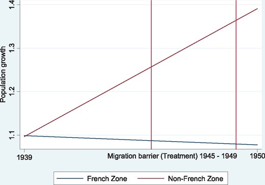
Population growth before and after the treatment.
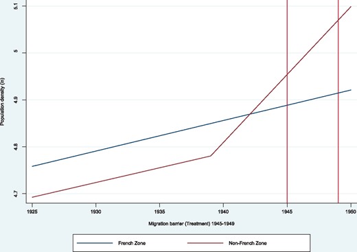
Population density before and after the treatment.
Selected regional differences among treated and non-treated regions
| Treated | Non-treated | Diff | |
|---|---|---|---|
| Population share of expellees in 1950 | 0.069 | 0.215 | *** |
| War-time destruction in 1945 | 0.187 | 0.157 | n.s. |
| Average price for renting a flat in 1950 (in Deutsch Mark) | 8.784 | 8.645 | n.s. |
| Unemployment rate in 1949 (in %) | 0.069 | 0.133 | *** |
Notes: N = 229 (N_French = 185; N_Non-French = 44); n.s., not significant.
p < 0.01.
As mentioned before, the inflow of expellees came along with a drastic deterioration of economic conditions. This is exemplified in Table 1 which shows that the unemployment rate in areas of the French occupation zone has been much lower than in non-French regions in December 1949. The housing conditions have been relatively similar. This shows that the official argument for the restrictive migration policy, namely above average war-related damages, is not supported by the statistics. Finally, the average price for renting a flat was not higher in areas formerly occupied by the French. In regions adjacent to the occupation zone border, the prices for flats have been even lower in areas formerly occupied by the French. Thus, lower costs of living and lower unemployment should have provided incentives to move to areas of the former French occupation zone once the migration barrier was no longer effective.
4.2. Baseline results
Table 2 presents the baseline results. The different model specifications clearly demonstrate that population growth after WWII was significantly lower in areas that were exposed to restrictive migration policies in the late 1940s. The effect is significant and negative for the period 1939–1946. The period from 1939 to 1950 includes the first year after the removal of the barrier. The coefficient estimate for the DiD estimator is only slightly smaller than in the 1939–1946 specification. The other models suggest that the coefficient is not getting smaller for time periods including years beyond 1961.15 Rather there is even a slight increase in the gap. In the early 1960s, the public resettlement policies were fading out which suggests that there was no adjustment of population levels beyond the direct effects of this scheme. The models of Table 2 show that war-time destruction in 1945 is negatively related to long-term growth.16 Distance to GDR and Czechoslovakia play no meaningful role.
The treatment effect of the migration barrier on population growth over time: the baseline model
| Dep Var: population growth (1925–1939) & (1939–X) | I | II | III | IV | V | VI | VII | VIII |
|---|---|---|---|---|---|---|---|---|
| 1939–1946 | 1939–1950 | 1939–1961 | 1939–1970 | 1939–1980 | 1939–1990 | 1939–2000 | 1939–2010 | |
| Post-1939 X | −0.318*** | −0.292*** | −0.170*** | −0.172*** | −0.210*** | −0.200*** | −0.212*** | −0.219*** |
| French Occ Zone | (0.029) | (0.025) | (0.028) | (0.045) | (0.057) | (0.064) | (0.071) | (0.081) |
| French Occ Zone (Y = 1) | 0.003 | 0.006 | −0.043 | −0.082* | −0.102* | −0.115** | −0.125* | −0.135* |
| (0.080) | (0.074) | (0.048) | (0.045) | (0.054) | (0.054) | (0.065) | (0.071) | |
| Post-1939 (Y = 1) | 0.381*** | 0.427*** | 0.381*** | 0.515*** | 0.603*** | 0.690*** | 0.844*** | 0.852*** |
| (0.022) | (0.021) | (0.021) | (0.031) | (0.046) | (0.053) | (0.063) | (0.073) | |
| War-time destruction 1945 | −0.988*** | −0.830*** | −0.368*** | −0.391*** | −0.457*** | −0.564*** | −0.686*** | −0.664*** |
| (0.082) | (0.070) | (0.070) | (0.102) | (0.134) | (0.147) | (0.175) | (0.187) | |
| Distance to GDR | 0.000 | −0.011 | −0.058* | −0.037 | −0.065 | −0.066 | −0.075 | −0.082 |
| (0.027) | (0.025) | (0.033) | (0.051) | (0.069) | (0.080) | (0.092) | (0.102) | |
| Distance to CSSR | 0.034 | 0.040 | 0.076** | 0.083 | 0.139* | 0.143* | 0.171* | 0.186* |
| (0.028) | (0.025) | (0.033) | (0.053) | (0.073) | (0.081) | (0.091) | (0.101) | |
| Population in t | −0.001*** | −0.001*** | −0.001* | −0.001** | −0.002** | −0.003** | −0.003*** | −0.003*** |
| (0.000) | (0.000) | (0.000) | (0.001) | (0.001) | (0.001) | (0.001) | (0.001) | |
| Controls for natural conditions | Y | Y | Y | Y | Y | Y | Y | Y |
| Planning region dummies | Y | Y | Y | Y | Y | Y | Y | Y |
| N | 458 | 458 | 458 | 458 | 458 | 458 | 458 | 458 |
| R2 | 0.743 | 0.773 | 0.741 | 0.697 | 0.642 | 0.663 | 0.694 | 0.671 |
Notes: Clustered standard errors (SE) (planning region * year). The controls for natural conditions comprise a dummy variable indicating a location at the coastline, soil indicators (topsoil parental material, topsoil organic carbon content, mineralogy of the subsoil) and slope.
p < 0.01,
p < 0.05,
p < 0.1.
There is also a treatment effect in models with population density as the outcome variable (Supplementary Table A3). With this outcome variable it is possible to test whether there was a common trend in development in treated and non-treated areas before the treatment became effective. The test requires an interaction of the dummy indicating the French occupation zone with a year dummy for 1925. The interaction is not significant. This indicates that French and Non-French areas were not different in terms of urbanization before the migration barrier treatment while urbanization is lower in treated areas after 1945 due to lower population growth.
4.3. Robustness checks
In a first robustness check, endogenous controls, as discussed in Section 3.3, are introduced (Table 3). In a further assessment, the baseline control variables are interacted with the year dummy for the second period to account for year-specific effects of these exogenous war-related and natural conditions (Supplementary Table A4). Both exercises leave the DiD estimators virtually unchanged.17
Robustness check I: extended models with further controls for regional conditions
| Dep Var: population growth (1925–1939) & (1939–X) | I | II | III | IV | V | VI | VII | VIII |
|---|---|---|---|---|---|---|---|---|
| 1939–1946 | 1939–1950 | 1939–1961 | 1939–1970 | 1939–1980 | 1939–1990 | 1939–2000 | 1939–2010 | |
| Post-1939 X | −0.317*** | −0.292*** | −0.174*** | −0.178*** | −0.216*** | −0.205*** | −0.216*** | −0.223*** |
| French Occ Zone | (0.029) | (0.026) | (0.028) | (0.045) | (0.058) | (0.065) | (0.072) | (0.083) |
| French Occ Zone (Y = 1) | 0.064 | 0.083 | 0.032 | 0.009 | 0.007 | 0.001 | −0.012 | −0.082 |
| (0.067) | (0.068) | (0.041) | (0.046) | (0.057) | (0.061) | (0.071) | (0.077) | |
| Post-1939 (Y = 1) | 0.363*** | 0.405*** | 0.353*** | 0.463*** | 0.523*** | 0.603*** | 0.743*** | 0.749*** |
| (0.025) | (0.024) | (0.023) | (0.035) | (0.047) | (0.051) | (0.061) | (0.068) | |
| War-time destruction 1945 | −0.997*** | −0.839*** | −0.378*** | −0.405*** | −0.471*** | −0.577*** | −0.697*** | −0.673*** |
| (0.083) | (0.070) | (0.067) | (0.095) | (0.127) | (0.140) | (0.168) | (0.181) | |
| Distance to GDR | 0.046 | 0.039 | 0.001 | 0.070 | 0.086 | 0.094 | 0.104 | 0.103 |
| (0.034) | (0.031) | (0.042) | (0.069) | (0.095) | (0.104) | (0.122) | (0.133) | |
| Distance to CSSR | 0.006 | 0.011 | 0.047 | 0.034 | 0.082 | 0.086 | 0.112 | 0.129 |
| (0.028) | (0.025) | (0.031) | (0.050) | (0.069) | (0.076) | (0.089) | (0.099) | |
| Population in t | −0.001** | −0.001** | −0.001*** | −0.001*** | −0.002*** | −0.003*** | −0.003*** | −0.003*** |
| (0.000) | (0.000) | (0.000) | (0.001) | (0.001) | (0.001) | (0.001) | (0.001) | |
| Market potential (ln) | 0.212 | 0.236* | 0.274* | 0.531** | 0.818** | 0.903** | 1.068** | 1.091** |
| (0.128) | (0.127) | (0.160) | (0.260) | (0.390) | (0.427) | (0.480) | (0.507) | |
| University (Y = 1) | 0.032 | 0.034 | 0.067*** | 0.112*** | 0.177*** | 0.189*** | 0.205*** | 0.230*** |
| (0.036) | (0.031) | (0.023) | (0.035) | (0.056) | (0.061) | (0.073) | (0.085) | |
| Employment share in manufacturing | −0.047 | 0.021 | 0.195** | 0.262** | 0.263 | 0.244 | 0.166 | 0.141 |
| (0.078) | (0.072) | (0.080) | (0.132) | (0.192) | (0.209) | (0.238) | (0.255) | |
| Nazi support | 0.366** | 0.356** | 0.271* | 0.469* | 0.444 | 0.357 | 0.235 | 0.128 |
| (0.151) | (0.145) | (0.155) | (0.241) | (0.310) | (0.325) | (0.373) | (0.401) | |
| Population share of men aged between 14 and 45 years old | 1.413** | 1.472** | 1.512** | 2.045** | 1.699 | 1.463 | 0.930 | 0.604 |
| (0.632) | (0.583) | (0.641) | (0.951) | (1.222) | (1.332) | (1.553) | (1.769) | |
| Controls Table 2 | Y | Y | Y | Y | Y | Y | Y | Y |
| N | 458 | 458 | 458 | 458 | 458 | 458 | 458 | 458 |
| R2 | 0.749 | 0.780 | 0.754 | 0.712 | 0.656 | 0.675 | 0.703 | 0.679 |
Notes: Clustered SE (planning region * year).
p < 0.01,
p < 0.05,
p < 0.1.
Further robustness checks aim at dispelling concerns that the results are driven by economically motivated and strategic decisions affecting where the borderline between the French and the other occupation zones was actually drawn. Schumann (2014) explains that the Southern border between the French and the US zone was deliberately placed such that the freeway linking Frankfurt and Munich remained under US control. As a consequence, the industrial region around Stuttgart was in the US zone, whereas some of the more peripheral neighboring counties were in the French zone. Furthermore, in the northern part of the French occupation zone for some regions, the border was partly determined by the Rhine River, which created a natural border between regions and limits commuting flows.18
In further robustness checks, regions adjacent to counties hosting the freeway linking Frankfurt and Munich as well as regions adjacent to the river Rhein are excluded to account for the abovementioned concerns (Supplementary Table A5). This exercise leaves the DiD estimators virtually unchanged although the precision of the estimate for growth in the period 1939 and 2010 is reduced eventually also due to lower case numbers in these models.
In the aftermath of the German division not only individuals relocated to West Germany but also firms (e.g. Falck et al., 2013). To the extent that their relocation was non-random different developments across zones may not only stem from the population shock. Such developments should be captured by planning region effects that control for labor market regions and the general economic environment for relocation choice.
In an additional robustness check, regions of the French occupation zone are matched to comparable regions in the zone of the UK and the USA. Applying a propensity score matching based on the variables used in the models of Table 3. There are 12 pairs of matched regions which means that almost 30 per cent of the regions of the French occupation zone have been matched.19 Despite the sharp reduction in case numbers, there is still a negative and significant treatment effect, which is doubling in size from 1950 to 2010 (Supplementary Table A6). There is obviously divergence in the growth patterns among regions that had similar regional conditions before the treatment. It should be noted that the planning regions where the matched non-treated regions are located are in close proximity to the French occupation zone border. Regions in labor market areas adjacent to the occupation zone border are likely to have similar unobserved regional characteristics which corroborate the validity of the conducted matching. Altogether, the additional analyses provide confidence in the baseline estimates presented in Section 4.2.
4.4. Population growth after removing the migration barrier
This section devotes attention to population growth after removing the migration barrier. To this end, the empirical strategy is slightly adapted. So far, the pre-treatment period from 1925 to 1939 has been included along with a post-treatment period from 1939 spanning to various years after 1945. Now, the period between 1939 and 1950 and the period from 1950 and later years are separated.
Model I of Table 4 includes the same control variables as in Table 2. The model shows a clear negative growth effect for the period 1939–1950 while there is a positive growth effect for the period 1950–1961. The DiD coefficient for the second 11-year period is only one third in absolute size of the negative growth in the period when the migration barrier was effective. In Model II, the post-1950 growth period is extended to the year 2010. The gap in the DiD coefficients hardly narrowed suggesting that there was no meaningful convergence.
Population growth before and after removing the migration barrier: main results
| Dep Va: population growth (1925–39); (1939–1950) & (1950–X) | I | II | III | IV | V | VI | VII | VIII |
|---|---|---|---|---|---|---|---|---|
| 1950–1961 | 1950–2010 | 1950–1961 | 1950–2010 | 1950–1961 | 1950–2010 | 1950–1961 | 1950–2010 | |
| Post-1939 X | −0.310*** | −0.310*** | −0.299*** | −0.298*** | −0.300*** | −0.302*** | −0.298*** | −0.299*** |
| French Occ Zone | (0.029) | (0.048) | (0.026) | (0.048) | (0.026) | (0.046) | (0.025) | (0.033) |
| Post-1950 X | 0.119*** | 0.143** | −0.269*** | −0.268*** | −0.273*** | −0.270*** | −0.244*** | −0.195*** |
| French Occ Zone | (0.025) | (0.066) | (0.033) | (0.075) | (0.033) | (0.073) | (0.039) | (0.072) |
| Controls Table 2 | Y | Y | Y | Y | Y | Y | Y | Y |
| Population share of expellees 1950 | N | N | −2.718*** | −2.881*** | −2.647*** | −2.441*** | −2.220*** | −1.292*** |
| (0.192) | (0.348) | (0.187) | (0.356) | (0.206) | (0.417) | |||
| Controls Table 4 | N | N | N | N | Y | Y | Y | Y |
| Expellee characteristics 1950 | N | N | N | N | N | N | Y | Y |
| Post-1950 migration flows | N | N | N | N | N | N | Y | Y |
| Observations | 687 | 687 | 687 | 687 | 687 | 687 | 687 | 687 |
| R2 | 0.564 | 0.422 | 0.738 | 0.525 | 0.748 | 0.569 | 0.779 | 0.672 |
Notes: Clustered SE (planning region * year). Expellee characteristics comprise the share of expellees from the former eastern German territories, the share of expellees from Czechoslovakia, the share of Protestants among expellees, the share of expellees in non-agricultural private sector self-employment and the share of expellees that are active in agriculture in 1950. Migration flows after the WWII are captured by the population share of East German refugees from the Soviet occupation zone in 1961, the share of expellees in 1961 that first located in the Soviet occupation zone before moving further to West Germany and the share of people from abroad in 1970.
p < 0.01,
p < 0.05.
Models I and II of Table 4 clearly show that the post-1950 population growth in the French occupation zone did not compensate for the lower growth of the 1939–1950 period. In Model III, the population share of expellees in 1950 is introduced. For 1925 and 1939, the variable assumes the value of zero while it has positive values for 1950. The share of expellees after the war was strongly correlated with bad housing conditions and unemployment.21 Thus, this share is an implicit control for incentives to re-migrate to other regions with more favorable economic conditions in the 1950s. As previously mentioned, there was also a public relocation scheme for expellees to regions with low initial population shares of expellees.22
The population share of expellees has a strong significant negative effect on population growth. This clearly indicates that many expellees indeed migrated to places with initially lower expellee shares. Against this background, it is remarkable that introducing the population share of expellees in 1950 implies a negative DiD coefficient for the post-1950 period that is almost equal in size as the respective coefficient for the period when the migration barrier was effective (Models III and IV). This pattern is robust when introducing endogenous variables like in Table 3 (Models V and VI). Models VII and VIII include characteristics of the regional expellee population and for in-migration of people from the Soviet occupation zone and from abroad (for details, see notes of Table 4).
The results of Table 4 are remarkable. If there was a return to the pre-war spatial equilibrium in terms of population levels one should expect that the DiD coefficient becomes insignificant when controlling for the population share of expellees because the initial regionally different population shock was caused by the inflow of expellees. Quite to the contrary, the analysis suggests that areas of the former French occupation zone attracted fewer expellees as to be expected based on the initially regionally different population shares of expellees.
The results of Table 4 raise the question of what determined population growth after 1950 and where did expellees move to. In the models of Table 5 growth dynamics until 1961 are analyzed which is the last year with regional information on expellees. In Model I of Table 5, the controls for war-related and natural conditions are interacted with year dummies for 1939 and 1950 to account for differential impacts of these factors during the first post-war years and the post-1950 period as compared to the pre-war years. Introducing the year-war destruction interactions reduces the 1950 DiD coefficient substantially (Table 5, Model I). Including the other year-interactions implies only a slight decrease in the coefficient which turns into insignificance (Model II). These patterns suggest that particularly war-time destruction is informative about migration behavior after 1950 and deserves a closer inspection.
Population growth after the removal of the migration barrier: selected patterns
| Dep Var: | I | II | III | IV | V | VI | VII | VIII |
|---|---|---|---|---|---|---|---|---|
| Population growth: 1925–1939; 1939–1950; 1950–1961 | Expellee growth 1950–1961 | Population growth (excl. expellees) 1950–1961 | ||||||
| French Occ Zone | Ref | Ref | 0.251 | 0.516* | 0.481* | −0.038 | −0.020 | −0.036 |
| (1925–39) | (1925–39) | (0.380) | (0.294) | (0.288) | (0.032) | (0.052) | (0.061) | |
| Post-1939 X | −0.292*** | −0.233*** | — | — | — | — | — | — |
| French Occ Zone | (0.026) | (0.032) | — | — | — | — | — | — |
| Post-1950 X | −0.084** | −0.051 | — | — | — | — | — | — |
| French Occ Zone | (0.036) | (0.036) | — | — | — | — | — | — |
| Controls Table 4 model VII/VIII | Y | Y | N | Y | Y | N | Y | Y |
| War-time destruction | Ref | Ref | 1.460*** | 0.846*** | 0.800*** | 0.214*** | 0.070 | 0.045 |
| (1925–39) | (1925–39) | (0.259) | (0.214) | (0.229) | (0.062) | (0.055) | (0.072) | |
| Post-1939 X War-time destruction | −0.832*** | −0.947*** | — | — | — | — | — | — |
| (0.071) | (0.094) | — | — | — | — | — | — | |
| Post-1950 X War-time destruction | −0.049 | −0.080 | — | — | — | — | — | — |
| (0.059) | (0.058) | — | — | — | — | — | — | |
| French Occ Zone X | N | N | N | N | 0.158 | N | N | 0.075 |
| War-time Destruction | N | N | N | N | (0.598) | N | N | (0.073) |
| Post-1950 X Natural conditions & Distance to CSSR/GDR | N | Y | — | — | — | — | — | — |
| Post-1950 X Natural conditions & distance to CSSR/GDR | N | Y | — | — | — | — | — | — |
| Observations | 687 | 687 | 229 | 229 | 229 | 229 | 229 | 229 |
| R2 | 0.808 | 0.842 | 0.896 | 0.937 | 0.937 | 0.809 | 0.869 | 0.870 |
Notes: Clustered SE (planning region * year). Instead of the size of the population in 1950 it is controlled for the number of expellees in Models III–V and for the number of non-expellees in Models VI–VIII.
p < 0.01,
p < 0.1.
The interaction between the post-1950 dummy and war-time destruction is insignificant. This implies that places with a lot of war-time destruction in the early 1940s were back on the same growth trend as before 1939 despite controlling for the population share of expellees in 1950 which was very low in places with a lot of destroyed housing (for details, see Section 3.3). The reconstruction of cities in the 1950s made it possible to relocate there. Models III–V show that it was particularly expellees that moved to cities in the 1950 to 1961 period. Comparing growth in expellee population with that of non-expellees reveals that the effect is seven times stronger for the former group when not considering endogenous controls (Models III and VI). Including the full range of controls as of Table 3 reveals that war-time destruction is not any longer statistically significantly related to the growth of non-expellees while results are robust for expellee growth although the coefficient is much lower (Model IV and VII). An interaction between war-time destruction and the marker for the French occupation zone is insignificant (Model V and VIII). The dummy indicating whether an area was part of the French occupation zone cannot be interpreted in the models of Table 5 because it is perfectly correlated with the planning region dummies.
Altogether, there have been two types of areas with low population shares of expellees after WWII, heavily destroyed cities and regions in the former French occupation zone that saw a severe migration barrier. While cities returned to their pre-war growth trend, areas exposed to the migration barrier did not. Overall, the findings of the analysis suggest that agglomerations have been more attractive for refugees.
Unfortunately, there is no regional data on the number of refugees beyond the year 1961. So, one can only speculate about the long-run consequences of the migration behavior in the 1950s. There might have been a spatial sorting of expellees into cities after 1950 that came with a delay due to war-time destructions. Typically, it is that particularly productive individuals migrate to agglomerations (e.g. Behrens et al., 2014). This sorting might have been conducive for the long-term development of cities and their returning to the pre-war growth trend. This would be in line with the earlier finding by Brakman et al. (2004) who show that post-war city growth trends in West Germany were not permanently affected by war-time destructions. Furthermore, people that already integrated themselves economically and socially in regions where they initially arrived may have been less likely to participate in the public relocation program that distributed expellees also to rural places in the former French occupation zone. Thus, there might have been a negative selection of expellees into the relocation program that implied that regions developed less successful as compared to places where particularly those expellees remained that were already economically and socially integrated. This explanation would be consistent with previous findings showing that high population shares of expellees after WWII promoted structural change toward more productive sectors in West Germany (Braun and Kvasnicka, 2014; Semrad, 2015).
4.5. The results against the background of previous research
Previous evidence by Schumann (2014) finds that there is still a striking difference between adjacent French and US areas in 1970 in terms of population levels. Braun et al. (2017) find that there is no effect until 1970 when the shock is assessed at the level of large labor market areas. This section attempts to put the findings of the current article into perspective and to reconcile contradicting findings. The results of Section 4.4 already give an idea that the population dynamics in cities (war-devastated regions) were different than in rural areas. This pattern cannot be addressed by the small sample of Schumann (2014) who exploits mainly municipalities in a specific spatial context nor by Braun et al. (2017) who have large regions where these different dynamics at a smaller regional level are likely to cancel out.
Splitting the sample at the median level of war-time destruction to run separate analyses for highly and moderately devastated areas provides further insights. For both sub-samples, there are different expectations regarding the treatment effect which follow the reasoning outlined at the end of the previous section. Immediately after WWII, agglomeration economies were ‘switched off’ since cities were heavily bombed. Cities were a very unattractive place due to the lack of housing. In the 1950s, the reconstruction of housing facilities of cities and in-migration from the overpopulated rural areas also implied that agglomeration economies prevailed which might have attracted further in-migration. Furthermore, the sorting and self-selection mechanisms described in Section 4.4 should be observable in all former occupation zones. However, cities in the French occupation zone may experience less inflow because there are (i) fewer expellees in the surrounding rural counties due to the previous migration barrier implying lower in-migration to nearby cities and because these cities are (ii) farther away for expellees in overpopulated rural areas in other occupation zones. Thus, there was a lower potential of population growth and accordingly prevailing agglomeration economies across cities in the former French occupation zone. These initially different conditions may have also created better conditions for the prevalence of agglomeration economies in the long run. Accordingly, one should expect no convergence for cities (heavily destroyed areas) in the short and in the long run. In rural (less destroyed) areas agglomeration, there should be convergence because there is less capacity for agglomeration economies.
Both expectations can be confirmed when splitting the sample in accordance to the level of war-time destruction (Table 6). For regions with an above-median level of destruction (e.g., regions with high population density, cities) there is a pronounced and lasting negative treatment effect of the French migration barrier which is even increasing over time. For regions with below-median war-time destruction, there is no long-term treatment effect. Some areas were heavily destroyed without being among the most densely populated regions. To err on the side of caution, a robustness check on regions that were above-median war devastated and had an above-median pre-war population density in 1939 confirms the main results (Supplementary Table A7).
The treatment effect of the migration barrier on population growth over time across regions with different degree of war-time destruction
| Dep Var: population growth (1925–1939) & (1939–X) | I | II | III | IV | V | VI | VII | VIII |
|---|---|---|---|---|---|---|---|---|
| 1939–1950 | 1939–1970 | 1939–1990 | 1939–1910 | 1939–1950 | 1939–1970 | 1939–1990 | 1939–2010 | |
| Panel A: Above-median war-time destruction | ||||||||
| Post-1939 X | −0.253*** | −0.262*** | −0.313*** | −0.354*** | −0.256*** | −0.276*** | −0.330*** | −0.374*** |
| French Occ Zone | (0.039) | (0.050) | (0.067) | (0.081) | (0.040) | (0.050) | (0.067) | (0.081) |
| Controls Table 4 | N | N | N | N | Y | Y | Y | Y |
| Observations | 230 | 230 | 230 | 230 | 230 | 230 | 230 | 230 |
| R2 | 0.680 | 0.739 | 0.735 | 0.751 | 0.690 | 0.759 | 0.752 | 0.764 |
| Panel B: Below-median war-time destruction | ||||||||
| Post-1939 X | −0.334*** | −0.042 | −0.039 | −0.034 | −0.332*** | −0.046 | −0.046 | −0.041 |
| French Occ Zone | (0.027) | (0.063) | (0.095) | (0.126) | (0.026) | (0.064) | (0.097) | (0.129) |
| Controls Table 4 | N | N | N | N | Y | Y | Y | Y |
| Observations | 228 | 228 | 228 | 228 | 228 | 228 | 228 | 228 |
| R2 | 0.841 | 0.726 | 0.671 | 0.670 | 0.845 | 0.740 | 0.688 | 0.688 |
Notes: Clustered SE (planning region * year).
p < 0.01.
Finally, it is checked whether these results hold when aggregating to the larger labor market areas which come close to the definition used by Braun et al. (2017). Table 7 confirms these results (Panel B and C). In addition, there is no long-term effect on average when not splitting the sample (Panel A). This is in line with the findings by Braun et al. (2017) who are using even larger regions in their analysis.23 One can conclude from this additional exercise that there is a negative treatment effect for regions where we should expect the prevalence of agglomeration forces while location fundamentals seem to matter in other areas. Overall, the results suggest that the impact of population shocks on the spatial distribution of population over time depends on the capacity of affected regions to unfold agglomeration economies in the long run.
The treatment effect of the migration barrier on population growth over time across planning regions (labor market areas)
| Dep Var: population growth (1925–39) & (1939–X) | I | II | III | IV | V | VI | VII | VIII |
|---|---|---|---|---|---|---|---|---|
| 1939–1950 | 1939–1970 | 1939–1990 | 1939–2010 | 1939–1950 | 1939–1970 | 1939–1990 | 1939–2010 | |
| Panel A: all regions | ||||||||
| Post-1939 X | −0.290*** | −0.155** | −0.108 | −0.097 | −0.287*** | −0.162** | −0.109 | −0.094 |
| French Occ Zone | (0.030) | (0.070) | (0.081) | (0.097) | (0.029) | (0.072) | (0.080) | (0.098) |
| Controls Table 4 | N | N | N | N | Y | Y | Y | Y |
| Observations | 138 | 138 | 138 | 138 | 138 | 138 | 138 | 138 |
| R2 | 0.765 | 0.521 | 0.756 | 0.748 | 0.774 | 0.545 | 0.770 | 0.755 |
| Panel B: above-median war-time destruction | ||||||||
| Post-1939 X | −0.219*** | −0.258*** | −0.313*** | −0.342*** | −0.212*** | −0.253*** | −0.306*** | −0.332*** |
| French Occ Zone | (0.038) | (0.070) | (0.091) | (0.111) | (0.040) | (0.076) | (0.098) | (0.122) |
| Controls Table 4 | N | N | N | N | Y | Y | Y | Y |
| Observations | 70 | 70 | 70 | 70 | 70 | 70 | 70 | 70 |
| R2 | 0.743 | 0.766 | 0.762 | 0.758 | 0.768 | 0.772 | 0.768 | 0.767 |
| Panel C: below-median war-time destruction | ||||||||
| Post-1939 X | −0.375*** | −0.049 | 0.181* | 0.241** | −0.379*** | −0.068 | 0.172* | 0.237* |
| French Occ Zone | (0.040) | (0.142) | (0.094) | (0.119) | (0.047) | (0.178) | (0.097) | (0.122) |
| Controls Table 4 | N | N | N | N | Y | Y | Y | Y |
| Observations | 68 | 68 | 68 | 68 | 68 | 68 | 68 | 68 |
| R2 | 0.841 | 0.592 | 0.843 | 0.837 | 0.857 | 0.648 | 0.882 | 0.861 |
Notes: Robust standard errors. The models include dummies for the states in which the planning regions are located.
p < 0.05,
p < 0.01.
4.6. Population and income growth
The previous sections showed that there is a long-term treatment effect of the migration barrier on the spatial distribution of the population. It is unclear inasmuch higher population growth relates to economic development. In Table 8, the dependent variable is the growth in income between 1925 and 2010. The historical data stem from the income statistics of the German Reich that were published at the level of regions in the year 1925 which is the only available pre-treatment year for income as a measure for economic development (Statistik des Deutschen Reichs, 1929). Current data are published regularly by the Federal Statistical Office (Destatis, 2018).
Population growth and change in income levels across regions
| Dep Var: income growth (1925–2010) | I | II | III | IV |
|---|---|---|---|---|
| Income level 1925 | −0.970*** | −0.898*** | −0.959*** | −0.893*** |
| (0.027) | (0.029) | (0.027) | (0.029) | |
| Population growth | 0.087*** | 0.082*** | 0.100*** | 0.092*** |
| (0.016) | (0.014) | (0.018) | (0.017) | |
| Population growth X | N | N | −0.071*** | −0.073*** |
| French Occ Zone | N | N | (0.027) | (0.026) |
| Controls regional conditions | Y | Y | Y | Y |
| Controls Table 2 | N | Y | N | Y |
| Observations | 229 | 229 | 229 | 229 |
| R2 | 0.934 | 0.952 | 0.937 | 0.953 |
Notes: Robust standard errors. The controls for regional conditions include the market potential, the employment share in manufacturing and the presence of a university in 1939.
p < 0.01.
The regression specification with income growth as outcome variables includes population growth, the initial level of income in 1925 as well as the controls for market potential, the regional share of manufacturing and the presence of a university before WWII. The historical degree of industrialization can be regarded as a very rough measure for investment in human and physical capital while universities partly capture the regional stock of knowledge. In all models, the population growth is positively related to income growth (Model I). This holds when adding controls for war-related impacts and natural conditions (Model II).
In Section 4.4, it was speculated that the in-migration into the French occupation zone after 1950 came along with a negative selection of expellees into the relocation program that implied that regions developed less successful as compared to places where particularly those expellees remained that were already economically integrated. If there was such a selection, this should also imply a lower contribution of population growth to increases in income levels. In the Models III and IV of Table 8 population growth is interacted with the dummy indicating being located in the French occupation zone. There is a negative and significant interaction effect which is almost equal in size of the main effect. Thus, there is a rather small positive relationship between population growth and changes in income levels in the former French occupation zone. This indicates that the population in-flow into the French occupation zone was partly driven by a negative selection.
5. Conclusions
This article analyzes the long-term effect of temporary but restrictive migration barriers on regional development in the wake of a refugee crisis by exploiting the large-scale expulsions of Germans after WWII. This empirical setting has several ‘appealing’ features that avoid methodological concerns (forced) migration research typically has to deal with. There were no selective migration and cohort effects influencing migrating decisions. The same applies to return migration as well as language and skill transfer. The article exploits the fact that some German regions did not accept the hostage of refugees. This was a political decision by French authorities responsible for administering a part of Germany after WWII. In contrast to the French occupation zone, refugees could resettle without political restrictions in the other two West German occupation zones (USA, UK), and in the Soviet occupation zone.
The results reveal that regions that were exposed to the migration barrier in the first years after WWII have significantly lower levels of population growth and population density until today while these areas had the same level of urbanization as other West German regions before the introduction of the migration barrier. The results are robust to controlling for an array of other factors that determined expellee resettlement and long-run development. There appears to be no convergence of population growth over time.
Assessing the dynamics of development after the removal of the migration barrier reveals spatial sorting patterns. There is a slight catch-up in population levels in areas of the former French occupation zone in the first years after removing the barrier. One can speculate that expellees were negatively selected into public relocation programs, namely that only people that were not yet economically and socially integrated in the regions where they initially arrived, participated in the scheme. Further analyses show that population growth in the former French occupation zone is to a lower degree related to growth in income levels as compared to other regions which suggest that the population inflow in these areas did contribute less to economic development.
The assessment also reveals a massive internal migration after 1950 into cities which were heavily bombed in WWII. Migration to the reconstructed cities was particularly driven by expellees. This migration pattern suggests that there was a delayed spatial sorting that could not take place earlier due to war-time destruction. Theory predicts that particularly highly productive people select into cities (e.g. Behrens et al., 2014). Positive and negative selection of expellees in the first years after WWII seems to explain that there was no return to the pre-war spatial equilibrium in terms of population levels. The empirical regularities found in this article also suggest that there is a negative treatment effect for regions where we should expect the prevalence of agglomeration forces while location fundamentals seem to matter in other areas.
Overall, the results indicate that the impact of population shocks on the spatial distribution of population depends on the capacity of affected regions to unfold agglomeration economies. Thus, also policies to deal with asymmetric population shocks depend on this capacity. This is an important insight especially for countries with a strong federal tradition where local development policy decisions are made at smaller regional scales. Moreover, the results of this study have also implications for policies on the spatial allocation of refugees. One can expect that refugees sort into places where they perceive themselves to be more productive after rules regarding compulsory residence in a region are fading out. The theory on spatial sorting (e.g., Behrens et al., 2014) would predict a surge into cities which, in the current refugee crisis, maybe even spurred if there are already enclaves of people with a similar ethnic origin (Edin et al., 2003).
The limitation of the study is that there is not much information on socio-demographic characteristics of expellees relocating after 1950. It would be helpful to understand who was selecting into migration to areas exposed to the treatment. This notwithstanding, the analysis demonstrates that temporary place-based migration barriers in the wake of a refugee crisis can have long-run negative implications for regional development.
Footnotes
1 There was also no barrier in the Soviet occupation zone which is not part of the empirical analysis here due to data constraints.
2 In a somewhat similar vein, Moser et al. (2014) find that Jewish émigrés who left Nazi Germany toward the USA had a positive impact on innovation and patent output.
3 For a discussion of selectivity of refugee migration, see Engel and Ibanez (2007). Studies on the economic integration of refugee versus economic migrants suggest that not only the former group is positively selected (Cortes, 2004; Dustmann et al., 2017b).
4 There are also micro studies on the economic integration of expellees (Falck et al., 2013; Bauer et al., 2013).
5 Based on a modified Solow-Swan growth model, one should expect that a lower rate of population growth implies a higher steady-state output per worker due to the capital dilution effect if expellees have no own capital which can be readily assumed.
6 A list of these regions can be obtained upon request.
7 An alternative would be to use the Federal States as clustering variable. However, state-by-time clustering would provide only 20 clusters instead of 140 planning region-by-time clusters. The validity of cluster-robust inference requires that the number of clusters is large (Cameron et al., 2008).
8 A correlation matrix is not reported for brevity.
9 Brakman et al. (2004) and Burchardi and Hassan (2013) use a different data source for war-time destruction which is less precise for the regional level of analysis used in this study.
10 Movements of expellees into West German regions that are close to the French occupation zone are affecting the post-1945 market potential as well.
11 Due to data constraint, for the year 1925 the population share aged above 15 years is used to capture the workforce.
12 In this campaign, anti-Semitic and other ideological components of the Nazi movement played an important role as compared to the last free elections in 1932 where many people voted for right-wing parties due to economic motives (Satyanath et al., 2014). The election data are based on the publicly available raw data as provided by Falter and Haenisch (1990). The share of right-wing votes in 1928 includes the number of votes for the DNVP (Deutsche Nationale Volkspartei) and the NSDAP (Nationalsozialistische Deutsche Arbeiterpartei) which is the party that emerged out of the ‘Hitler movement’. The years 1925 and 1939 that are considered in the analysis assume the same values per region.
13 Men that were in their adolescents below the age of 18 years in 1939 were likely to be conscripted in the last years of the war. For the year 1925, the same values as for 1939 have to be assumed because there is no data on adult population in specific age brackets.
14 For the latter group, there is only reliable information from the census in 1970.
15 One can track population development over the 1950s when referring to data from respective Yearbooks of the German Federal Statistical Office. However, the definition of expellees is slightly different in these years. It also includes Germans coming from communist Eastern Germany.
16 It should be noted that there is only variation in this variable for the periods starting in 1939.
17 The models of Table 3 show that there is a robust positive relationship between long-run population growth with pre-war market potential and the existence of a university. Agglomeration effects play an important role for regional growth (e.g., Glaeser et al., 1992; Behrens et al., 2014). The treatment effect remains robust when introducing population density. It has to be noted that pre-war population density is highly correlated with war-time destruction (r = 0.68). There is also a positive effect for the control variable on pre-war support for the Nazi regime in models that span the period 1925–1950. The share of men in conscription-prone age groups has a positive effect on growth in models that span the period 1925–1970. Areas with a high share of men in this age group and high levels of support for the regime might have been prospering before the war. Both regions may have also seen a huge inflow of people after the war either due to higher war-devastation in places with higher Nazi support or due to higher casualties in places with more men in conscription-prone age.
18 This conjecture is partly questionable as the BBSR, the Federal Institute for Research on Building, Urban Affairs, and Spatial Development, officially defines, for example, the planning region of Koblenz as including regions west and east of the river Rhein. Planning regions are labor market areas defined by frequent commuting flows within the area.
19 The algorithm is based on a standard nearest neighbor matching. The results are robust when playing around with different sets of baseline variables for the matching variables albeit the number of matched pairs varies accordingly.
20 The results of Table 2 showed that the treatment effect for the period 1939–1946 is almost similar to the DiD estimator for the 1939–1950 specification. Thus, there have been no huge population movements into the French occupation zone taking place between 1946 and 1950.
21 The correlation between the population share of expellees and the share of expellees living in emergency accommodations (Notunterkuenfte) was r = 0.78, while it is also highly correlated with local unemployment rates (r = 0.56).
22 The available data do not allow disentangling the migration flow of expellees that was due to quotas and those that were outside this system.
23 The original classification by Braun et al. (2017), which is based on Regierungsbezirke, is too large to perform the reconciling analyses.
References
Statistik des Deutschen Reichs (
Statistisches Bundesamt (
