


Abstract
Theory and evidence suggest that people born in different countries complement each other in the labor market. Immigrant diversity could augment productivity by enabling the combination of different skills, ideas and perspectives, resulting in greater productivity. Using matched employer–employee data for the USA, this paper evaluates this claim, and makes empirical and conceptual contributions to prior work. It addresses the potential bias from unobserved heterogeneity among individuals, work establishments and cities. The paper also identifies diversity impacts at both city and workplace scales, and considers how relationships vary across different segments of the labor market. Findings suggest that urban immigrant diversity produces positive and nontrivial spillovers for U.S. workers. This social return represents a distinct channel through which immigration may generate broad-based economic benefits.
1. Introduction
Since 1960, global flows of international migrants have more than doubled, alongside considerable growth in the mix of locations from which they hail (Özden et al., 2011). Much of this upswell in immigrant diversity is concentrated in cities in rich countries. In the USA, which attracts one in five international migrants, nearly 40% of the population in large metropolitan areas like New York and Los Angeles was born abroad, more than twice the national average. Outside of the USA, London, Hong Kong and other large metropolitan regions report similar levels of foreign-born residents and immigrant-derived heterogeneity. Smaller, and less famously cosmopolitan cities are also increasingly attracting a wide range of foreign-born workers, and consequently becoming more demographically diverse.
This paper aims to determine whether this diversity affects worker productivity. Theory—drawn from psychology, sociology, economics and geography—suggests a double-edged relationship rooted in externalities in production. Whether good or bad, the starting point is the assumption that country of birth signals distinctiveness in peoples’ heuristics. On the positive side, interactions among a heuristically heterogeneous population widen the scope of available solutions. On this basis, immigrant diversity can generate spillovers that raise worker productivity. On the negative side, co-operation among workers from different backgrounds presents challenges, resulting in higher transaction costs that can reduce productivity.
Based on the conjecture that economically significant interactions among a diverse populace need not occur solely inside work teams and organizations, empirical researchers have examined the links between diversity and productivity at the metropolitan scale, considering city systems in the USA, UK, EU15, Germany, Australia and the Netherlands. Quite consistently, researchers find that cities featuring more diverse urban workforces have higher levels of wages, rents and employment, suggesting net positive productivity spillovers from immigrant diversity (e.g., Ottaviano and Peri, 2006; Nathan, 2011; Kemeny, 2012; Bellini et al., 2013; Suedekum et al., 2014; Trax et al., 2015).
The present article makes four main contributions to this growing literature. First and foremost, it aims to produce the strongest available evidence regarding the existence of spillovers from immigrant diversity in the U.S. cities. In order to generate high-quality evidence, we seek to overcome issues of nonrandom worker selection that are present in nearly all extant studies, addressing the possibility that highly productive workers are drawn to cities that are immigrant-diverse. In this regard, it responds to an open question about the importance of these sorting dynamics in measuring diversity spillovers: of the two known papers addressing this issue empirically, Bakens et al. (2013) find that scant spillovers remain after accounting for sorting on unobservables in the Netherlands, whereas in the German context, Trax et al. (2015) find a continuing positive association between regional cultural diversity and plant productivity. We do not yet know how selection dynamics might affect prior estimates produced for the USA, including seminal work by Ottaviano and Peri (2006). Second, this paper adds value by exploring whether spillovers from diversity emanate chiefly from within individual establishments, or from the broader metropolitan scale, what Jane Jacobs’ poetically described as the ‘ballet of the good city sidewalk’ (Jacobs, 1961, 50). Third, considering studies by Borjas (2003), Card (2007) and Lewis and Peri (2014) that highlight how modest aggregate immigration impacts can conceal substantial variation across the wage distribution, this paper examines whether benefits or costs derived from immigrant diversity depend on one’s position in the labor market. Last, it aims to distinguish whether any benefits derived from diversity are driven by heterogeneity across the entire labor market, as opposed to diversity only among workers at the top. We formalize these issues in the following research questions:
For the average urban worker, does the immigrant diversity present in one’s city or workplace generate productivity externalities?
Are such spillovers unevenly distributed among workers occupying different segments of the labor market?
Who generates spillovers from immigrant diversity? Is it diversity among all workers, or among only those occupying higher labor market segments?
To answer these questions, we make use of the U.S. Census Bureau’s confidential Longitudinal Employer-Household Dynamics (LEHD), a uniquely comprehensive matched employer–employee dataset of U.S. workers and their work establishments. The version of LEHD used covers nearly all employees in 29 states, on a quarterly basis starting, for some states, in 1991 and continuing through 2008. We adapt an approach for the identification of urban externalities in production suggested by Moretti (2004b) who leverages the panel dimension of our data. We estimate fixed effects models over a sample of urban workers who hold multi-year work ‘spells’ in the same establishment and city, thereby accounting for stationary unobserved heterogeneity at individual, work establishment and city level. Individual earnings are used as a proxy for productivity, and key predictors are indicators of birthplace diversity measured at both metropolitan and workplace levels. Hence, we estimate how workers’ wages change in response to changes in the diversity in the cities where they live, as well as in the establishments where they work. We pursue two strategies to account for potential bias from unobserved shocks that might simultaneously shift workers’ wages as well as diversity levels. First, we estimate the importance of several dynamic measures capturing local labor demand. Second, we generate generalized method of moments (GMMs) estimates, using lags of metropolitan and establishment diversity as instruments.
We find a robust positive relationship between earnings and both city- and workplace-specific manifestations of immigrant diversity. This positive association is materially unchanged with the inclusion of assorted control variables, including measures that account for changes in immigrants’ human capital. Results are consistent across various subsamples, including ones that focus narrowly on tradable activities, bolstering the claim that the link between diversity and wages reflects a productivity effect, rather than being driven by immigration-related quality-of-life factors. They remain consistent across a range of different approaches to the measurement of diversity. IV and other robustness checks suggest that findings are not driven by changes in local demand conditions or other unobserved shocks. Overall, the evidence supports the idea that immigrant diversity raises worker productivity, and that benefits flow from one’s broader urban context as well as one’s workplace.
We also find consistent estimates of spillovers for workers in each wage quartile. We interpret this to mean that the benefits of diversity are equally shared across the entire labor market. However, spillovers emanate chiefly from workers holding high-wage jobs. At the city scale, diversity is only significantly related to wages when measured among workers at the higher end of the wage distribution; meanwhile, workplace diversity emerges as uniformly positively and significantly, but coefficients are considerably larger when diversity is measured only across such high-wage workers.
To provide a sense of the magnitudes of diversity spillovers for the average worker, our baseline model (Table 2, Model 3) suggests that, all else equal, a one standard deviation increase in city immigrant diversity is associated with a 5.8% increase in wages. At the same time, a one standard deviation increase in workplace immigrant diversity raises wages by 1.6%. Over the study period, the average metropolitan area experiences an increase in diversity corresponding to half a standard deviation, although in 15% of cities, immigrant diversity increased by more than a standard deviation. The confirmation of city effects supports the existing scholarship, though city effects in the present paper are more modest than for approaches that have not accounted for sorting, workplace characteristics and other hard-to-observe factors.
The remainder of the paper is organized in five sections. Section 2 reviews the literature motivating this study. Section 3 lays out the empirical approach. Section 4 describes the data. Section 5 presents results. Section 6 concludes.
2. Existing literature
Much of the public debate and academic research on the economic impacts of immigration has focused on answering a question fraught with political and economic significance: how will growing flows of immigrants—and in particular relatively low-skill immigrants—affect job market outcomes of native-born workers (Borjas, 1994, 1995; Card, 2001, 2005)? While debates over negative substitution effects continue (cf. Borjas, 2015; Peri and Yasenov, 2015), recent findings leveraging detailed individual and firm-level data suggest that immigrants and natives can also be thought of as complements, with positive, albeit relatively modest wage benefits (Ottaviano and Peri, 2012; Dustmann et al., 2013; Lewis and Peri, 2014). Another strand of this recent work shows how immigrant entry in labor markets prompts natives to shift occupations, with generally positive outcomes measured in terms of wages and employment (Peri and Sparber, 2009; Cattaneo et al., 2013; Ortega and Verdugo, 2014; Foged and Peri, 2016).
The current paper examines a specific dimension of the relationship between immigration and economic welfare. It asks: how might a labor force including immigrants born in a wide range of countries perform differently from one that is more homogeneous? Scholars examining this question directly have theorized and sought empirical support for a link between immigrant diversity and innovation, entrepreneurship and productivity.1 The outcome of interest in this article is productivity, and thus the remainder of this section reviews that strand of the literature.
Organization-focused research spanning such fields as psychology, organizational sociology, artificial intelligence and economics suggests that interactions among individuals from diverse backgrounds could either augment or inhibit productivity. On the positive side, theorists argue that the experience of having been born in a particular location shapes one’s worldview (Hong and Page, 2004). It follows that, relative to more homogeneous sets of people, groups consisting of individuals from diverse birthplaces ought to contain an enlarged pool of available perspectives and heuristics. This heuristic diversity ought to improve problem solving in two ways. First, it will map out a larger proportion of the potential solutions available in the total problem space. Second, it will raise the likelihood of generating innovations by recombining ideas (Aiken and Hage, 1971; Nisbett et al., 1980; Hong and Page, 2001, 2004). On the other hand, psychology’s ‘social identity theory’ suggests that diversity can inhibit productivity. A long line of studies find that teams straddling cultural divides can find it hard to generate trust and to effectively co-operate (e.g., Byrne, 1971; Harrison and Klein, 2007; Van Knippenberg and Schippers, 2007).
Although such arguments were initially made with individual organizations and work teams in mind, they also map neatly onto the urban scale. A wealth of theory and empirics suggests that problem solving and knowledge production depend upon interactions that extend beyond atomized organizations—whether they arise in the context of formal partnerships or serendipitous, informal exchanges; it is widely understood that such ‘external’ interactions tend to have a local, metropolitan character (Jacobs, 1969; Jaffe et al., 1993; Feldman and Audretsch, 1999; Storper and Venables, 2004). At this scale, it makes sense to think about diversity as potentially generating location-specific externalities—indeed they could be described as a specific form of social returns to human capital. Similar to the wealth of studies indicating local spillovers from education (for instance: Rauch, 1993; Moretti, 2004a, 2004b), the present article, and ones like it, explores local spillovers from immigrant diversity.
Using public-use data from the 2007 American Community Survey (ACS), Figure 1 presents the motivating stylized fact: U.S. cities in which the average worker is highly paid also feature greater immigrant heterogeneity (using the common fractionalization index measured over birthplace). Researchers have sought to address a variety of substantive and methodological concerns in order to determine whether this simple bivariate correlation reflects an underlying relationship running from diversity to productivity.
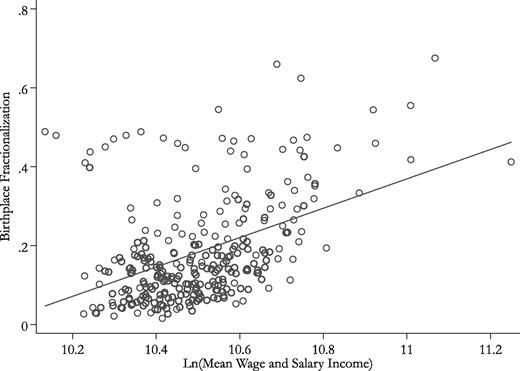
U.S. metropolitan wages and birthplace fractionalization, 2007. Notes: Data come from a 2007 1% public-use sample of the ACS (Ruggles et al., 2010). Points on the scatter plot reflect actual city values for wages and diversity, whereas the solid line reflects the least-squares fitted regression line. Fitted equation: Log (city average of annual wage and salary income) = 0.372 (Birthplace Fractionalization) −3.724; R2 = 0.194.
A wide range of empirical studies find a consistently positive and largely significant relationship between regional immigrant diversity and worker productivity. The seminal reference is Ottaviano and Peri (2006), who jointly test the relationship between diversity and wages and rents across U.S. metropolitan areas. They find that birthplace diversity is positively and robustly correlated with both outcomes, which they interpret as signaling that diversity raises productivity. Similar tests in other advanced economies also detect a positive relationship (Nathan, 2011; Kemeny, 2012; Ager and Brückner, 2013; Bakens et al., 2013; Bellini et al., 2013; Longhi, 2013; Suedekum et al., 2014; Trax et al., 2015; Elias and Paradies, 2016). And yet these studies leave key issues unresolved, inhibiting our ability to make confident statements about the underlying relationship between diversity and productivity. Most significant among these unresolved issues are nonrandom selection or sorting, longitudinal dynamics and firm and workplace heterogeneity.
Sorting refers to the idea that workers select into cities based on underlying features, some of which may be both (a) unmeasured and (b) correlated with immigrant diversity and wages. One plausible version of this idea states that immigrant-diverse cities may also draw highly skilled workers (skilled in ways that are not apparent from easily measurable characteristics like educational attainment). Researchers have mostly used models in which it is assumed that workers are homogeneous except for their birthplace, education and a relatively modest range of other observable factors. For example, Ottaviano and Peri (2006) consider the relationship between birthplace diversity and wages for white male native-born workers between the ages of 40 and 50 years. But their approach cannot address the likely scenario that, even among members sharing these features, unobserved differences in preferences and abilities exist that affect both individual productivity and locational choices (for discussion of this issue in immigration-impacts research, see: Lewis and Peri, 2014). Highly productive workers may select into high-diversity cities because they have particular preferences for amenities that flow from diversity (Florida, 2002); alternately, such sorting could be part of a process by which workers match their abilities to places with a particular industrial mix or position on quality ladders (Combes et al., 2008; Kemeny and Storper, 2012; Moretti, 2013). Whatever the cause, the presence of nonrandom selection is likely to generate upward bias in estimates of the relationship between diversity and productivity.
To the best of our knowledge, to date only two studies of spillovers from immigrant diversity have directly addressed this issue. Trax et al. (2015) leverage panel data on German plants, and find a positive and statistically significant relationship between total factor productivity and city- and plant-level cultural diversity. Bakens et al. (2013) exploit an individual-level panel of wages and rents in Dutch cities, using a two-step process that first separates individual-, sector- and city-level contributions to wages and rents, and second identifies the importance of city diversity in shaping outcomes of interest. Although they demonstrate a positive correlation between diversity and wages, coefficients on diversity are mostly insignificant. The Netherlands is particular in terms of its geographical scale and city size distribution, but the disjuncture between this finding and prior work highlights the potential importance of unobservable characteristics in determining how diversity may be related to economic outcomes of interest.
Another issue is that studies examining regional economies have largely ignored the scale of the workplace. This is a problem in the general sense of failing to account for the ways in which characteristics of firms and individual establishments are important for understanding variation in productivity (Haltiwanger et al., 1999). But it also raises a particular issue in the context of spillovers from immigrant diversity: we have little understanding of the scale at which any productivity-augmenting interactions might be occurring. The earliest scholarly focus on diversity considers impacts in organizations and the work teams inside them. Meanwhile, city-focused researchers consider that regions are the appropriate containers bounding the relevant economic interactions. But of course birthplace-diverse cities are likely to feature birthplace-diverse business establishments. Hence, what looks like a ‘Jane Jacobs’-style metropolitan effect might properly be an organizational one; depending on study design, the reverse could also be true. Or there may be productivity effects operating simultaneously within organizations and at the metropolitan scale.
Only a handful of empirical articles seek to tease out these effects. In addition to the article by Trax et al. (2015) which we describe above, Nathan (2015) considers the influence of ethnic diversity in British cities and firms’ top management teams, and finds mixed evidence that they are related to sales. More loosely related, Lee (2013) finds a small, positive relationship between the foreignness of UK firm managers (rather than their diversity) and firm process and product innovation, but he finds no significant effect of the share of foreign-born in the overall regional population. More work is needed to clarify the role of diversity at these different scales.
A further challenge to the current empirical literature is the paucity of studies exploring longitudinal dynamics. Urban immigrant diversity varies across cities, but it also varies within them across time. If it is the case that diversity directly influences productivity, then shifts in the former should be reflected in changes in the latter. Among the few studies addressing the potentially dynamic nature of this relationship, Longhi (2013) finds that the positive relationship between diversity in English Local Authority Districts and workers’ wages found in cross-sections (consistent with much of the existing research) disappears in panel estimates. This contrarian finding suggests the importance of examining this relationship in a dynamic framework.
Equally underexplored is how diversity operates across a heterogeneous labor force. Despite recent work on immigration highlighting the possibility that modest aggregate welfare effects conceal substantial variability across the labor market (Borjas, 2003; Card, 2007; Ottaviano and Peri, 2012; Lewis and Peri, 2014), most studies of diversity report only effects for the average worker. Although the idea of competition between less-skilled immigrants and natives looms large in academic studies (Borjas, 2015, 2016), a growing body of research, some of which exploits detailed individual- and firm-level data sources, suggests that immigrants, and especially immigrants further up the skill continuum, act predominantly as complements to native-born workers (Cortés and Tessada, 2011; Ottaviano and Peri, 2012; Cattaneo et al., 2013; Dustmann et al., 2013; Kerr, 2013; Lewis and Peri, 2014; Peri and Yasenov, 2015; Foged and Peri, 2016). Such studies suggest the importance of exploring potential segment-specific regularities in the elasticity of substitution, as well as dynamic complementarity across different labor market segments. However, we know of no paper that explores how the effects of diversity depend on one’s position in local labor markets.
Just as segment-specific differences generate heterogeneity in how immigrants affect natives’ labor market outcomes, diversity measured among specific subsets of workers may be differently associated with worker productivity. Particularly as the theorized mechanism explaining diversity’s positive impact rests on a particular kind of complementarity—of backgrounds and therefore of perspectives, we need a stronger understanding about how this may vary systematically across the labor market. One angle to pursue is whether diversity across workers at higher and lower ends of the labor market contribute equally to the generation of any productivity spillovers. If one assumes that high-wage or highly skilled workers are more likely to engage in complex problem solving, it is plausible that spillovers arise only from diversity among such workers, rather than from diversity measured across the entire labor force. To our knowledge, Suedekum et al. (2014) is the only paper to address this theme. Their findings suggest that the benefits of immigrant diversity do not emerge only or even mainly from the skilled immigrant population. Instead, controlling for the share of foreign-born immigrants in German urban cities, both high- and low-skill immigrant diversity generate spillovers that augment productivity among local natives.
3. Empirical approach
Concerns about sorting and longitudinal dynamics can be addressed by estimating models relating diversity and productivity over a large-N, large-T panel of individuals. Differencing the wages of individuals over time addresses bias arising from sorting driven by unobserved heterogeneity, as long as relevant individual characteristics are stationary. Panel data also permit observation of how diversity moves in relation to individuals’ wages. To answer questions regarding the scale at which spillovers arise, data on individuals must be supplemented with information about the birthplace composition of each workplace and urban region.
Applying the fixed effects estimator, Equation (1) explores how an individual’s wage responds to changes in the level of immigrant diversity around her, while it accounts for major sources of spurious correlation that might otherwise bias estimates. Over a full sample of workers, Equation (1) provides estimates of diversity spillovers for the average worker, but it can be easily adapted to answers of our second and third research questions. To identify differences in who benefits from overall levels of city- and workplace diversity—our second research question—we generate estimates for samples of workers restricted to individual city-specific wage quartiles.2 Addressing the third question, djt and dpjt refer to diversity measures generated for a specific quartile of a city or workplace wage distribution, as opposed to measures based on all workers at either scale. The aim in this case is to reveal if the relationship between diversity and productivity originates among workers occupying specific segments of the labor force.
Following the standard spatial equilibrium setup, one might seek to match a model predicting wages based on Equation (1) with another predicting rents. Explained formally in Ottaviano and Peri (2006), we briefly remind readers of the logic here. In a national system of cities in which workers are relatively free to make locational choices, diversity’s effects may not be confined to the sphere of production. Although wages are broadly taken to signal productivity, diversity in this context could also function as an amenity that workers value (or not) as an object of consumption. This has potential implications for factor prices, in terms of the wages workers are willing to accept, as well as the costs they face in the housing market, and relatedly, on their locational choices. Among urban economists, it is commonly assumed that inter-urban differences in workers’ real utility—a function of nominal wages as well as housing costs and location-specific amenities—ought to be driven toward equalization by the mobility of workers (Rosen, 1979; Roback, 1982; Glaeser and Gottlieb, 2009). In the current context, this formalizes the idea that immigrant diversity could also shape welfare by influencing available amenities, which will likely be capitalized into housing costs. Thus, jointly interpretating the relationships between diversity and wages as well as diversity and rents allows for a better understanding of whether rising wages signal actual productivity increases or compensation for reduced quality-of-life.
Yet related work on spillovers from education suggests a simpler approach. Acemoglu and Angrist (2001) and Moretti (2004a) argue that, in areas containing firms selling goods and services beyond their immediate locality, higher nominal wages must indicate higher average worker productivity. While firms in nontradable activities may reference local prices, traded-goods firms face national prices. If they paid higher wages with no compensating productivity advantages, firms would be forced to relocate to cities offering some form of compensating differential—whether in the form of cheaper land or higher quality-of-life. Based on this rationale, models of diversity and wages like Equation (1), estimated over a population of firms that includes those engaged in tradable activities, can plausibly shed light on local productivity effects. This is the approach we take.
Another concern in estimation is whether annual earnings effectively gauge productivity. Although imperfect, wages are widely considered to be the best available indicator of worker productivity (Feldstein, 2008), being less subject to measurement error than output estimates from the Census of Manufactures (Ciccone and Hall, 1996). In an urban context, rising productivity is likely to be expressed in higher wages (Combes et al., 2005), and establishment level productivity and wages exhibit similar elasticities with respect to city size (Combes et al., 2010). Still, given wage stagnation over the study period, in our reliance on wages as a proxy we assess a greater risk of generating a Type II error; or less severely, we might underestimate the strength of the relationship between diversity and productivity. Given the results reported in Section 5, the second of these concerns seems more plausible than the first.3
To capture the effects of diversity on worker productivity, the main identifying assumption to be satisfied is that the return on unobserved worker ability in their establishment and city is stationary over time, or at least that changes are uncorrelated with changes in city-specific diversity. As in Moretti (2004a), this return need not be general across higher-order categories, in this case establishments and cities.
4. Data
To estimate Equation (1), we use data from the U.S. Census Bureau’s confidential LEHD Infrastructure files, available in the Federal Statistical Research Data Centers, administered by the Bureau’s Center for Economic Studies. The LEHD program integrates administrative records from state-specific unemployment insurance (UI) programs with Census Bureau economic and demographic data, providing a nearly universal picture of private sector jobs in the USA (McKinney and Vilhuber, 2014). The LEHD has poorer coverage for agricultural workers and Federal parts of the public sector. Even so, LEHD captures at least 90% of civilian jobs (McKinney and Vilhuber, 2014, 7–2). The version of the data available for this study covers 29 states with observations starting as early as 1991 and going through 2008.4
Our strategy depends on being able to assign workers both to work establishments and to Metropolitan Core-Based Statistical Areas (CBSAs) that reflect economically integrated urban regions.5 We need to assign workers to cities in order to measure metropolitan immigrant diversity and decide who is in and out of the sample. We must also identify each individual’s work establishment in order to produce establishment-level diversity measures, as well as other salient workplace characteristics. For workers in jobs at single-unit firms (firms with only one plant, outlet or office), knowing the employer tells you the place of work, because there is only one possible location. However, for workers employed at multi-unit firms, knowing the employer cannot always definitively reveal the place of work. About 30–40% of workers included in the LEHD data files work at multi-unit firms (McKinney and Vilhuber, 2014). To produce the Quarterly Workforce Indicators, LEHD researchers have built a file (the Unit-to-Worker file, or U2W) that, for each person employed in a multi-unit firm, provides 10 work-unit imputations. Imputations are based on distance between workers’ homes and establishment locations, and the distribution of employment across the establishments within the multi-unit employer, leveraging actual establishment–worker data which is available only for the state of Minnesota to generalize to the remainder of states (McKinney and Vilhuber, 2014, see Chapter 9). Because the number of observations is so large and the place of work location structures much of the data processing necessary for our estimation strategy (building diversity measures; determining which workers are in and out of the sample; linking city and establishment characteristics to individual workers in the panel) using the multiple imputations is impractical. Instead, for each job in a multi-unit employer, we assign each worker to their most frequently imputed establishment (the mode), using random assignment among tied modal units.6
Once the multi-unit workers are assigned to a single establishment, we link variables stored in LEHD infrastructure files to individuals and their work places. We capture workplace features including location, total annual employment and NAICS industry; as well as worker characteristics like place of birth, sex and race, and the length of work spells in each workplace. Following a common practice in the literature, we limit the age range of workers to be over 16 and less than 66 years old. Together, these variables allow us to build annual city- and establishment-level diversity measures; generate person- and establishment-level characteristics and to construct a panel of workers with multi-year job spells in a single location.
To construct metropolitan diversity measures, we first narrow our list of CBSAs to those that do not cross state boundaries with states unavailable to our project. Thus, although jobs located in Newark, NJ are included in our raw data, we drop them because they are part of the CBSA for New York City that also includes jobs in New York State and Pennsylvania, to which we do not have access. We do include CBSAs straddling multiple states to which we do have access, such as Texarkana in Texas and Arkansas. Our final sample includes 163 CBSAs.7 With the list of metropolitan areas determined, we calculate several alternative measures of birthplace diversity based on all individuals in the LEHD data who worked in a CBSA in a given calendar year.
We measure establishment-level diversity by considering the mix of workers in each establishment. When measuring diversity in workplaces, instead of weighting each person’s contribution to birthplace diversity evenly as we do in the city measures, we weight each person’s contribution depending on how many quarters they work in a particular establishment. If they worked half the year in one establishment and half the year in another, then they count as half a person in the diversity measures of each establishment for that year.
Our analytical strategy relies on relating annual changes in wages with changes in the city and workplace diversity. To accomplish this we focus on people who remain in a single city and in a single establishment as others move in and out of both, changing the level of diversity around the stayers. Thus, our analytical sample includes fewer people than those who contributed to the city- and establishment diversity measures, since we keep only workers with multi-year job spells in a single workplace. Specifically, it is a panel of individual workers, tracking their wages in a single job spell of at least two continuous calendar years in one establishment. To construct this, we calculate annual wages from the reported quarterly wages, trimming years without positive earnings in all four quarters.
Additionally, we exclude workers with wages below the 5th percentile of the wage distribution, on the basis that LEHD’s inclusion of all workers earning at least one dollar in a quarter captures some very low earners perhaps operating under irregular employment situations. We also restrict the sample to jobs at establishments with at least 10 employees, in order to be able to generate meaningful workplace-specific diversity estimates. And we drop workers who are simultaneously employed in multiple jobs, so that we can clearly identify the source of any establishment-specific diversity effects. For each worker, we track only their longest job spell in any city in our sample, so an individual only shows up in one establishment and one city in the panel, even if they have multiple job spells over their observed career that meet the two-year minimum. These choices limit our ability to apply our results to certain parts of the American work force—for example, those with extremely tenuous labor market attachment or very low wages, and those who consistently hold multiple UI-covered jobs—but here we explicitly prioritize internal over external validity.
4.1. Diversity measures
Because it is the most widely used measure in the field, in much of the proceeding analysis, we estimate metropolitan as well as establishment-specific levels of diversity using the fractionalization index, using the universe of LEHD-coded worker birthplaces in a metropolitan area or work unit.9
Motivated by similar concerns, Ozgen et al. (2013) advocate using measures of depth and breadth in conjunction: the simple proportion of foreign born in the workforce, alongside a standard fractionalization index that is estimated over only the foreign-born population. Like the Alesina index, this approach has the virtue of being able to tease out the extent to which effects arise due to the sheer presence of foreign born, as distinct from their heterogeneity. Unlike an index estimated over the entire population, the immigrant-only fractionalization measure will not be influenced by the single large group of native workers in each city and establishment. However, since it cannot account for the likelihood of actually meeting and interacting with those from other groups, estimates using this measure include the share of foreign born in all workers as a control.
4.2. Individual-level measures
Our primary outcome of interest is an individual’s annual earnings. Wage data in LEHD come from UI records, and are measured here in log form. Average annual earnings are a little over $35,000 USD. Given a fixed effects approach, other available individual-level information in LEHD cannot be directly included in estimation as controls. Nonetheless, this information is useful to describe our sample. As Table 1 describes, the average worker in our sample is 40 years old. Sixty-seven percent of the sample is white, 84% is native born and 47% is female. These characteristics closely match the broader U.S. economy (Lee and Mather, 2008; Social Security Administration, 2015). The average work spell in the sample lasts nearly 5 years.
Summary statistics
| Variable | Mean | Standard deviation |
|---|---|---|
| Individual characteristics | ||
| Log annual earnings | 10.48 | 0.637 |
| Age | 40.32 | 11.67 |
| White | 0.667 | 0.471 |
| U.S. born | 0.840 | 0.366 |
| Female | 0.467 | 0.499 |
| Spell duration | 4.970 | 3.304 |
| Establishment characteristics | ||
| Birthplace fractionalization | 0.220 | 0.207 |
| Foreign born | 0.061 | 0.147 |
| Employment | 63.01 | 278.39 |
| Multi-unit | 0.349 | 0.477 |
| Manufacturing | 0.091 | 0.287 |
| City characteristics | ||
| Birthplace fractionalization | 0.180 | 0.129 |
| College share, all workers | 0.256 | 0.074 |
| College share, natives | 0.261 | 0.073 |
| College share, immigrants | 0.273 | 0.129 |
| Employment (10,000s) | 47.20 | 88.29 |
| Birthplace entropy | 0.563 | 0.317 |
| Birthplace Alesina | 0.011 | 0.017 |
| Birthplace fractionalization, immigrants | 0.819 | 0.182 |
| Share foreign born | 0.101 | 0.084 |
| Race fractionalization | 0.433 | 0.137 |
| Age fractionalization | 0.977 | 0.001 |
| Individuals | 33,550,000 | |
| Establishments | 1,193,000 | |
| CBSAs | 163 | |
4.3. Establishment-level controls
In addition to workplace-specific immigrant fractionalization, we also capture annual changes in establishment employment levels. We include employment based on the rationale that changes in aggregate workforce size can influence productivity through economies of scale. The average establishment in our sample employs 63 workers. In terms of other broad characteristics of our sample, Table 1 shows that 6% of jobs are held by foreign-born workers, while 35% of establishments are part of multi-unit firms. Nine percent of these units are chiefly engaged in manufacturing activities.
4.4. Metropolitan-level controls
In addition to indicators of metropolitan birthplace diversity, a variety of city-level characteristics are included in the regression results that follow. In each model, we include indicators of local externalities from scale and education. Measures of CBSA employment are included to capture the effects of agglomeration economies (Lewis and Peri, 2014). To measure education levels, we estimate the annual share of each CBSA’s workforce holding at least a 4-year college degree, using 5% public-use IPUMS extracts from the 1990 and 2000 Decennial Censuses, as well as 1% samples from each year of the 2001–2008 ACS (Ruggles et al., 2010).11 Among other city-level controls, motivated by related work on other forms of heterogeneity (e.g., Sparber, 2010; Østergaard et al., 2011), we use LEHD data to calculate additional diversity-based sources of externalities, based on city-specific variation in age and race.
5. Results
This section presents estimates of the relationship between birthplace diversity and wages. As described in Section 3, results are produced using fixed effects models on an annual panel of workers over their longest job spell during the study period (1991–2008). Each model includes a fixed effect that eliminates bias from stationary unobserved heterogeneity among workers, their establishment and their city. Year dummy variables are included to capture unmeasured shocks that are uniform across workers, plants and cities, but which vary over time. Throughout, standard errors are clustered at the establishment level, on the basis that wages are likely to be most strongly non-independent within workplaces.
5.1. Diversity spillovers for the average worker
Table 2 presents initial estimates of the relationship between immigrant diversity and wages for the full sample of workers. Column 1 presents results for city-level birthplace fractionalization alone, controlling for the metropolitan proportion of college-educated workers, and metropolitan and workplace employment. This model relates directly to the extant urban literature, by considering the operation of the independent variable of interest at the city level only. At the same time, it improves upon prior work, chiefly by accounting for stationary unobserved heterogeneity at multiple scales, while also controlling for changes in wages that might be due to shifts in establishment size. The coefficient on city immigrant diversity is positive and significant at a 1% level. As expected, control variables are all significant and positively related to wages. The coefficient on the share of college-educated workers is similar to that reported by Moretti (2004b), indicating that a 1% increase in the share of college-educated workers in a city yields a wage premium of just over 1%. Overall, the model yields the insight that, all else equal, workers in U.S. cities featuring larger annual increases in birthplace fractionalization also experienced larger annual wage growth. This conforms to much of the prior work, adding new evidence that earlier findings were not fully driven by unobserved, sorting-driven worker characteristics, nor by unmeasured permanent features of either establishments or cities.
Spillovers from immigrant diversity: main fixed-effects estimates
| Dependent variable: log of annual earnings | ||||||
|---|---|---|---|---|---|---|
| (1) | (2) | (3) | (4) | (5) | ||
| City measures | ||||||
| Birthplace fractionalization | 0.406*** | 0.375*** | 0.411*** | 0.390*** | ||
| (0.067) | (0.065) | (0.067) | (0.066) | |||
| College share | 0.164*** | 0.213*** | 0.162*** | 0.155*** | ||
| (0.040) | (0.041) | (0.040) | (0.040) | |||
| Employment (millions) | 0.032*** | 0.031*** | 0.031*** | 0.030*** | 0.030*** | |
| (0.005) | (0.006) | (0.005) | (0.005) | (0.005) | ||
| Race fractionalization | −0.043 | |||||
| (0.037) | ||||||
| Age fractionalization | 2.091 | |||||
| (1.433) | ||||||
| Native college share | 0.040 | |||||
| (0.036) | ||||||
| Immigrant college share | 0.072*** | |||||
| (0.009) | ||||||
| Establishment measures | ||||||
| Birthplace fractionalization | 0.079*** | 0.073*** | 0.073*** | 0.072*** | ||
| (0.008) | (0.007) | (0.007) | (0.007) | |||
| Employment (thousands) | 0.006* | 0.006* | 0.006* | 0.006* | 0.006* | |
| (0.003) | (0.003) | (0.003) | (0.003) | (0.003) | ||
Note: Standard errors in parentheses, corrected for clustering by establishment. Estimated equation is (1). R2 equal to 0.95 in all models. Year and individual × workplace × city fixed effects included in each model. Each model is estimated over 166,540,000 observations, nested in 33,550,000 individuals. Overall observation counts are rounded to the nearest 10,000 to ensure confidentiality.
*p < 0.10, **p < 0.05, ***p < 0.01.
Column 2 of Table 2 presents estimates of a model where fractionalization measured at the establishment level is the primary predictor of interest, and where we exclude city-level diversity. The coefficient on workplace diversity is positive and significant at a 1% level. Controls remain significant and consistent from the previous model. Interestingly, once exponentiated, the effect size of the share of college-educated workers in a metropolitan area is nearly identical to that found in Column 1 (1.24% for Column 2 where there is no measure of city diversity, versus 1.20 for Column 1 that includes such a diversity measure), further supporting the notion that immigrant diversity and education represent distinct channels for spillovers from human capital.12 Column 3 presents results in which we include measures of both city and establishment diversity. When included in the same specification, diversity at each scale is positively and significantly related to wages, though each coefficient is modestly smaller with the inclusion of the other. These results suggest that there are positive diversity impacts to be felt both from living in a more birthplace-diverse city, as well as from working in a more birthplace-diverse establishment.
The models in Columns 4 and 5 of Table 2 include some additional control variables. Model 4 adds measures of race and age fractionalization, to test whether immigrant diversity captures other aspects of heterogeneity that might be driving the result. Race and age diversity do not enter significantly into this model, and coefficients for immigrant diversity remain consistent. Column 5 presents results in which the city-level measure of the proportion of college-educated workers is disaggregated to capture the share of college educated among native-born, and separately foreign-born workers. Our aim is to ensure that any effects ascribed to immigrant heterogeneity do not instead reflect changes in the stock of human capital specific to the immigrant population (cf. Hunt and Gauthier-Loiselle, 2010; Paserman, 2013). Measures of education among natives and foreign born are each positively related to wages, though only the coefficient on immigrant college share is statistically significant. Most importantly, the inclusion of these measures does not materially affect the direction, magnitude or significance levels of the immigrant diversity variables.
We next probe the robustness of the results presented thus far. Specifically, we test whether findings are sensitive to the use of different measures of diversity; to the particular decisions made in constructing our analytical sample and to approaches that account for unobserved shocks at either the city or establishment level. Each of these issues is explored in turn.
Table 3 reports estimates in which we substitute several alternative measures of metropolitan immigrant heterogeneity for our main birthplace fractionalization measure. Because the control variables remain stable, we present condensed results, showing results only for diversity at each scale, with each row of the table indicating a separate model in which we use a particular measure of city-specific immigrant diversity. The first row reports estimates produced using the birthplace entropy measure described in Equation (3), whose strength lies in improved measurement under the quite plausible conditions that population subgroups are of different sizes. The coefficient on the entropy measure is positive and significant at a 1% level, and controls continue to display the expected signs and statistical significance. Rows 2 and 3 report results of two different approaches to explore the extent to which results derived from the standard fractionalization index are driven by the simple share of foreign born. In row 2, the Alesina diversity index enters as positively and significantly related to wages. Row 3 reports estimates in which we explicitly distinguish between the overall presence of nonnatives and diversity among those nonnatives, following Ozgen et al. (2013) and Nijkamp and Poot (2015). Controlling for the presence of foreign-born workers, birthplace diversity within the pool of a city’s immigrants remains positively and significantly associated with wages. Interpreting the economic significance of these various diversity indicators in relation to wages suggests that results are not especially sensitive to one’s choice of measure. Specifically, effect sizes for a one standard deviation change in city diversity are approximately 6% for the entropy index, 8% for the Alesina index and 9% for immigrant-only fractionalization.
Robustness: FE models with alternative city-specific diversity measures
| Dependent variable: log of annual earnings | ||
|---|---|---|
| Diversity coefficients | ||
| City (β) | Estab. (γ) | |
| (1) With city birthplace entropy | 0.161*** | 0.070*** |
| (0.025) | (0.007) | |
| (2) With city birthplace Alesina | 1.703*** | 0.070*** |
| (0.225) | (0.008) | |
| (3) With city birthplace immigrant-only Frac. | 0.403*** | 0.068*** |
| (0.036) | (0.008) | |
Notes: Each numbered row presents estimates for a single model, containing city-level education and employment controls, as well as a workplace-level measure of employment. Year and individual × workplace × city fixed effects included in each model. Standard errors in parentheses, corrected for clustering by establishment. Estimating equation is (1). R2 equal to 0.95 in all models. Each model in this table is estimated over 166,540,000 observations, nested in 33,550,000 individuals. These observation counts are rounded to the nearest 10,000 to ensure confidentiality.
*p < 0.10, **p < 0.05, ***p < 0.01.
We turn next to particular subsets of the main sample which, in different ways shed light on the relationship of interest. Results in Table 4 are from models that are directly comparable to those found in Column 3 in Table 2 in that each includes the usual controls as well as measures of immigrant fractionalization at both city and work unit scales. The first numbered row of Table 4 addresses concerns that measures of diversity may not be meaningful in small workplaces. The estimates reported are produced over a sample of workers holding jobs in establishments that have at least 20 employees. Coefficients for city- and establishment-diversity remain positive and statistically significant at a 1% level, and are closely comparable to estimates for the entire sample.
Robustness: FE models on selected subsamples of workers and establishments
| Dependent variable: log of annual earnings | ||||
|---|---|---|---|---|
| Fractionalization coeffs. | Counts (millions) | |||
| City (β) | Estab. (γ) | Observations | Individuals | |
| (1) Larger establishments only | 0.362*** | 0.081*** | 151.53 | 30.38 |
| (0.071) | (0.010) | |||
| (2) Single-unit firms only | 0.547*** | 0.079*** | 81.96 | 16.66 |
| (0.089) | (0.009) | |||
| (3) Native-born white males only | 0.502*** | 0.079*** | 59.02 | 11.34 |
| (0.079) | (0.009) | |||
| (4) Manufacturing plants only | 0.740*** | 0.114*** | 29.61 | 5.49 |
| (0.170) | (0.014) | |||
Notes: Each numbered row presents estimates for a single model, containing city-level education and employment controls, as well as workplace-specific employment, and year and individual × workplace × city fixed effects. Standard errors in parentheses, corrected for clustering by establishment. Estimated equation is (1). R2 equal to 0.94 in all models. Overall observation counts are rounded to the nearest 10,000 to ensure confidentiality. Larger plants in row 1 are those with at least 20 employees. Natives in row 3 are white male workers born in the USA.
*p < 0.10, **p < 0.05, ***p < 0.01.
The second row of Table 4 aims to determine whether or not the process of imputation of workers to establishments in multi-unit firms generates bias. This process could incorrectly assign some workers to establishments, and to a lesser extent to cities; in turn, this could bias measures of diversity, while also incorrectly relating other workplace characteristics to that particular worker. Row 2 of Table 4 presents estimates generated solely for the subset of employees working for single-unit firms. For these workers, there is only one possible place of work, thus we are confident we have each worker placed among the correct co-workers in the workplace. Results remain consistent: increased diversity at both the city and workplace level is positively and significantly related to increased wages. These results raise our confidence that our process for assigning multi-unit employees to work locations is not spuriously driving results.
Model 3 in Table 4 estimates the relationship between diversity and wages for white, native-born, male workers, in keeping with the main focus of much of the broader literature on the economic impacts of immigration. It is often contended that foreign-born workers displace and exert negative wage pressure on natives in the labor market, and especially native males. This subgroup has also been the focus of selected research on immigrant diversity, as a strategy for limiting worker heterogeneity within the analytical sample (for instance: Ottaviano and Peri, 2006; Kemeny, 2012). As with all of the previous models discussed, coefficients for diversity at each scale are positively and significantly linked to worker wages.
The final model in Table 4 aims to more deeply probe spatial-equilibrium concerns that the association between diversity and wages may indicate that diversity affects quality-of-life, not productivity. Since, due to data limitations, we cannot more directly capture the co-movement of changes in diversity and individual rents, we rely on the argument that changes in wages in a local economy that feature industries serving a national market must reflect changing productivity, otherwise the firms would be forced to relocate. Although Moretti (2004b) contends that the argument holds for wages if the local economy includes any national-serving or tradable products and services, in this model we interpret the point conservatively, limiting our model to a subset of activities that is certainly facing national (and even global) price competition: manufacturing. Model 4 presents results with the sample restricted to only workers in establishments classified within two-digit NAICS headings 31, 32 and 33. As in all of the previous models, city and workplace diversity emerge as positive and significant. Hence, the positive relationship between diversity and wages holds among workers about whom we are most confident that increased wages reflect increased productivity.
We turn next to addressing concerns about endogeneity. Although our baseline empirical approach aims to account for bias from worker selectivity into plants and metropolitan areas, interpretation remains vulnerable to the possibility that unobserved shocks at the level of the city or workplace may be driving the relationships of interest. We seek to address such concerns in two ways: (1) by considering the potential role of local demand shocks and (2) by instrumenting for city- and workplace-specific immigrant diversity.
Concerned with the fact that measures of employment growth may imprecisely capturing shocks, our second gauge of local demand conditions uses information from the Bureau of Labor Statistics’ Job Openings and Turnover Survey (JOLTS). JOLTS is based on surveys of over 16,000 nonagricultural firms conducted since 2001, and describes industry-specific national monthly unmet demand by listing unfilled jobs for which firms are actively recruiting. CBSA- and year-specific measures of job openings are constructed by weighting nationally representative two-digit NAICS JOLTS data with city-specific shares of employment by industry. We then divide this indicator by a measure of CBSA-specific unemployment, constructed by summing county-level estimates derived from the BLS Local Area Unemployment Statistics program.13
To match the availability of the JOLTS data, the first three models in Table 5 report results estimated on a sample restricted to job spells that occur between 2001 and 2008. Model 1 is a reference model with the standard controls but no demand shifters, offering a comparison for results generated over the restricted time period. Coefficients for workplace and metropolitan diversity are positive and significant at a 1% level, though they are smaller than for those produced for the full study period. Model 2 presents coefficients of interest in a model that includes the JOLTS-derived demand shifter. Although the demand shock measure enters significantly in the model, the size of the coefficient on city diversity is only modestly reduced, and both workplace and city diversity remain comparable in terms of sign and significance. Model 3 reports estimates that include the Bartik demand shifter. As expected, the Bartik measure is positively and significantly related to wages. But, the inclusion of this indicator does not materially change the relationship between wages and diversity measured at either the city or workplace scale.14
Robustness: demand shocks and instrumental variables
| Dependent variable: log of annual earnings | ||||
|---|---|---|---|---|
| Fractionalization coeffs. | Counts (millions) | |||
| City (β) | Estab. (γ) | Observations | Individuals | |
| (1) Baseline model 2001–2008 | 0.192*** | 0.037*** | 92.3 | 22.6 |
| (0.069) | (0.005) | |||
| (2) With JOLTS demand shock | 0.176*** | 0.037*** | 92.3 | 22.6 |
| (0.069) | (0.005) | |||
| (3) With Bartik demand shock | 0.198*** | 0.038*** | 92.3 | 22.6 |
| (0.068) | (0.005) | |||
| (4) GMM FE IV (1991–2008) | 0.432*** | 0.058*** | 15.89 | 3.24 |
| (0.144) | (0.013) | |||
Notes: Each numbered row presents estimates for a single model, containing city-level education and employment controls, as well as workplace-specific employment. Standard errors in parentheses, corrected for clustering by establishment. Observation counts are rounded to the nearest 10,000 to ensure confidentiality. Columns (1)–(3) estimated over 2001–2008; R2 greater than 0.96 in Columns (1)–(3). Model 4 estimated over 1991–2008, on a 30% random sample of individuals in the main analytical sample of ‘stayers’. Instruments used in this model are 3- and 4-year lags of city-level diversity, and 1-year lags of establishment-level diversity. Model 4 generated Kleibergen–Paap LM (underidentification) of 1.5e + 04 (p = 0.000) and a Hansen J of 0.045 (p = 0.83).
*p < 0.10, **p < 0.05, ***p < 0.01.
To further account for bias from dynamic unobserved heterogeneity, we also generate estimates using instrumental variables. In seeking suitable instruments, the strengths of the primary estimation strategy turn into liabilities. Simply, it is extremely difficult to find annually available candidate instruments for individual workplaces and cities that are sufficiently strong predictors of differences in immigrant diversity at the relevant level, and which are also plausibly orthogonal to unobserved shocks. Given the scarcity in LEHD of variables capturing workplace-specific characteristics, the challenge is most acute at the establishment scale. After rejecting several ‘external’ instruments, we subjected a multitude of lags of city and establishment immigrant diversity to tests of exclusion, under- and overidentification.15 An instrument set featuring three- and four-year lags of city diversity and one-year lags of establishment diversity passed these hurdles. Due to the nesting of individual workers inside establishments, we opt for cluster-robust GMM-FE IV, as this approach ought to produce more efficient estimates than conventional standard two-stage least squares (Baum et al., 2003).
Model 4 of Table 5 reports our instrumental variables estimates, produced for the full study period from 1991. To reduce computational intensiveness to a manageable level, estimates are produced on a 30% random sample of individuals from the main analytical sample, covering job spells for over three million workers. Instruments pass the Kleibergen–Paap underidentification test, indicating their relevance, though a large test score suggests that, despite the deeper lags, the instruments may be ‘too good’—too closely related to the potentially endogenous regressor. As the estimating equation is overidentified, we test for the joint orthogonality of the excluded instruments, using the Hansen J test statistic; results indicate that the instruments are independently distributed of the error process and that they are properly excluded from the model. The second-stage results shown in Model 4 broadly support non-instrumented findings. Diversity at the metropolitan scale is positively and significantly related to wages, as diversity is estimated at the establishment level. Coefficients for both key independent variables of interest remain close to those produced using the standard fixed effects estimator reported in Tables 2–4. These findings, even with less-than-perfect instruments, are consistent with cross-sectional studies using other IV strategies (e.g., Ottaviano and Peri, 2006; Kemeny, 2012).
Although we cannot fully eliminate the possibility that unmeasured shocks to cities and workplaces are driving the relationships between diversity and productivity, the evidence presented in Table 5 is consistent with the interpretation that the results in this paper are not driven by such shocks. They offer support for the idea that immigrant diversity in cities and work establishments generate wage-augmenting productivity spillovers.
5.2. Who benefits from spillovers from immigrant diversity?
In this section, we seek an answer to our second research question: are spillovers from immigrant diversity unevenly distributed among workers occupying different segments of the labor market? As described in Section 3, to investigate this question we begin by splitting our analytical sample into four groups. Workers are assigned to quartiles based on where they stand in their CBSA’s wage distribution. Equation (1) is then estimated separately for the subsample of workers in each quartile. The top panel of Table 6 presents results from models that include the usual controls, individual × establishment × city fixed effects, and standard errors clustered at the establishment level. Models 1–4 present results for workers in progressively higher quartiles of their city’s wage distribution. Across each of these models, coefficients for city-specific and establishment-specific immigrant diversity remain positively related to wages at a 1% level of significance. Magnitudes for city diversity coefficients are relatively stable, with formal tests indicating no statistically significant differences across quartiles.16 Coefficients for establishment-level diversity are also consistent across quartiles, with the exception of the highest wage quartile, where the social returns to rising workplace diversity are significantly larger in statistical terms, though substantively the differences are modest. Overall, we interpret the results in the top panel of Table 6 to indicate that productivity benefits from immigrant diversity are more or less evenly shared across the entire earnings spectrum.
Estimates of spillovers from immigrant diversity by wage quartile
| Dependent variable: log of annual earnings | ||||||
|---|---|---|---|---|---|---|
| Fractionalization coeffs. | Counts (millions) | |||||
| City (β) | Estab. (γ) | Observations | Individuals | R2 | ||
| FE estimates | ||||||
| (1) Wage quartile 1 (lowest) | 0.436*** | 0.069*** | 51.57 | 11.90 | 0.86 | |
| (0.058) | (0.004) | |||||
| (2) Wage quartile 2 | 0.384*** | 0.040*** | 42.30 | 8.44 | 0.83 | |
| (0.086) | (0.007) | |||||
| (3) Wage quartile 3 | 0.347*** | 0.062*** | 37.92 | 6.97 | 0.83 | |
| (0.099) | (0.013) | |||||
| (4) Wage quartile 4 (highest) | 0.414*** | 0.139*** | 34.65 | 6.23 | 0.89 | |
| (0.123) | (0.018) | |||||
| GMM FE IV estimates | ||||||
| (5) Wage quartile 2 | 0.539*** | 0.025 | 4.08 | 0.830 | – | |
| (0.178) | (0.015) | |||||
| (6) Wage quartile 3 | 0.408** | 0.046** | 4.06 | 0.795 | – | |
| (0.179) | (0.019) | |||||
| (7) Wage quartile 4 (highest) | 0.492*** | 0.123*** | 3.74 | 0.750 | – | |
| (0.181) | (0.026) | |||||
Notes: Each numbered row presents estimates for a single model, containing city-level education and employment controls, as well as workplace-specific employment, and year and individual × workplace × city fixed effects. Standard errors in parentheses, corrected for clustering by establishment. Overall observation counts are rounded to the nearest 10,000 to ensure confidentiality. GMM FE IV results not shown for wage quartile 1, as instruments were not found that passed exclusion restrictions, underidentification and overidentification tests. Instruments used include: 3- and 4-year lags of city-level immigrant diversity, and 1-year lags of establishment diversity. Results in models 5–7 are produced on a 30% random subsample of our primary analytical sample. Tests of Model 5 yielded Kleibergen–Paap LM (underidentification) of 1.1 + e04 (p = 0.000) and a Hansen J of 0.299 (p = 0.58). Tests of Model 6 yielded Kleibergen–Paap LM (underidentification) of 8722 (p = 0.000) and a Hansen J of 0.394 (p = 0.53). Tests of Model 7 yielded Kleibergen–Paap LM (underidentification) of 7428 (p = 0.000) and a Hansen J of 0.173 (p = 0.68).
*p < 0.10, **p < 0.05, ***p < 0.01.
When we instrument for immigrant diversity at the city and establishment scales, results are broadly supportive of this conclusion. The lower panel of Table 6 presents two-stage GMM FE IV estimates, with deeper lags of diversity used as instruments. For quartiles 2–4 we find combinations of lags that satisfy the exclusion restriction; we are unable to do so for the lowest wage quartile. Models 5–7 in Table 6 present estimates that instrument for city and workplace immigrant diversity using a combination of three- and four-year lags of metropolitan diversity, and a one-year lag of establishment diversity. As above, to avoid convergence problems in estimation, results are produced on a 30% random subsample of our primary analytical sample. These models pass tests of under and overidentification. The coefficient for city immigrant diversity is positively and significantly related to wages across each of the wage quartiles for which results are produced. Although somewhat larger, magnitudes are broadly comparable to those in the upper panel. Instrumented and uninstrumented coefficients on the establishment diversity variable are also similar, however the coefficient is only statistically significant for wage quartiles above the median.
Although incomplete, our IV estimates strengthen confidence in the idea that the benefits of diversity are spread across the wage distribution. This is clearest for spillovers from diversity at the metropolitan scale, while within establishments benefits appear to be concentrated among those occupying higher rungs of the ladder. It is worth noting that, due to the sampling strategy and the use of lagged instruments, results generated using GMM FE IV are drawn from a much more restricted sample than many of the other models presented earlier in this article, including the upper panel of Table 6. We recognize tradeoffs in privileging instrumented over uninstrumented estimates. Although results are broadly similar, for precision we prefer estimates reported in the upper panel.
5.3. Who generates spillovers from immigrant diversity?
While the previous section investigated whether diversity’s benefits are spread evenly across the labor force, we now turn to this article’s third and final question: who generates these spillovers? Specifically, we seek to determine whether the benefits from diversity emanate from the full pool of workers in a workplace or city, or rather, from diversity within particular subgroups. On the intuition that variation might be related to hierarchy in the labor market, we build an additional series of birthplace fractionalization measures that describe heterogeneity among low-wage, and separately, high-wage workers. To capture low-wage urban immigrant diversity, for each year and CBSA, we calculate the level of birthplace fractionalization present among workers with wages below the 25th percentile of their city’s wage distribution. High-wage urban immigrant diversity is measured in an analogous way for workers at or above the 75th percentile. Using a similar approach, we also build measures of low- and high-wage immigrant diversity at the establishment level, using wage distributions specific to each workplace.17
The top panel of Table 7 presents estimates based on a variant of Equation (1), predicting the relationship between a worker’s earnings and the immigrant diversity present among workers who belong to the least-well paid quartile of their city and workplace. As with the immediately previous tables, each row in Table 7 summarizes results for a distinct model estimated on a particular group of workers. Model 1 is estimated on the full analytical sample. Models 2–5 are estimated on progressively higher quartiles of the CBSA-specific wage distribution. Results across all of these models are consistent. In each, the coefficient for low-wage urban birthplace fractionalization is not statistically significant. Meanwhile, we find a consistent positive and significant relationship between wages and low-wage diversity at the workplace scale, though coefficients are roughly an order of magnitude smaller than typical estimates for establishment immigrant diversity measured over the entire workforce (i.e., Model 3 in Table 2). Overall, absent a significant link between wages and city-level diversity among low-wage workers, we conclude that the benefits described in relation to rising metropolitan immigrant diversity do not emanate from heterogeneity among a city’s lowest-paid workers.
Estimates of spillovers from immigrant diversity by wage quartile
| Dependent variable: log of annual earnings | ||||||
|---|---|---|---|---|---|---|
| Fractionalization coeffs. | Counts (millions) | |||||
| City (β) | Estab. (γ) | Observations | Individuals | R2 | ||
| FE estimates—low-wage birthplace diversity | ||||||
| (1) All workers | 0.007 | 0.009*** | 166.44 | 33.54 | 0.95 | |
| (0.047) | (0.001) | |||||
| (2) Wage quartile 1 (lowest) | 0.017 | 0.008*** | 51.57 | 11.90 | 0.86 | |
| (0.037) | (0.001) | |||||
| (3) Wage quartile 2 | 0.018 | 0.004*** | 42.30 | 8.44 | 0.83 | |
| (0.063) | (0.001) | |||||
| (4) Wage quartile 3 | −0.036 | 0.008*** | 37.92 | 6.97 | 0.83 | |
| (0.072) | (0.002) | |||||
| (5) Wage quartile 4 (highest) | 0.084 | 0.023*** | 34.65 | 6.23 | 0.89 | |
| (0.090) | (0.004) | |||||
| FE estimates—high-wage birthplace diversity | ||||||
| (6) All workers | 0.819*** | 0.056*** | 166.44 | 33.54 | 0.95 | |
| (0.044) | (0.003) | |||||
| (7) Wage quartile 1 (lowest) | 0.813*** | 0.062*** | 51.57 | 11.90 | 0.86 | |
| (0.047) | (0.002) | |||||
| (8) Wage quartile 2 | 0.715*** | 0.051*** | 42.30 | 8.44 | 0.83 | |
| (0.055) | (0.003) | |||||
| (9) Wage quartile 3 | 0.858*** | 0.045*** | 37.92 | 6.97 | 0.83 | |
| (0.046) | (0.005) | |||||
| (10) Wage quartile 4 (highest) | 0.873*** | 0.061*** | 34.65 | 6.23 | 0.89 | |
| (0.088) | (0.007) | |||||
| GMM FE IV estimates—high-wage birthplace diversity | ||||||
| (11) Wage quartile 2 | 0.570*** | 0.049*** | 3.06 | 0.640 | – | |
| (0.161) | (0.014) | |||||
| (12) Wage quartile 3 | 0.876*** | 0.045*** | 4.06 | 0.795 | – | |
| (0.143) | (0.018) | |||||
| (13) Wage quartile 4 (highest) | 0.747*** | 0.508*** | 4.89 | 0.950 | – | |
| (0.160) | (0.235) | |||||
Notes: Each numbered row presents estimates for a single model, containing city-level education and employment controls, as well as workplace-specific employment, and year and individual × workplace × city fixed effects. Standard errors in parentheses, corrected for clustering by establishment. Overall observation counts are rounded to the nearest 10,000 to ensure confidentiality. GMM FE IV results in models 11–13 are produced on a 30% random subsample of our primary analytical sample. Instruments used include: 3- and 4-year lags of city-level immigrant diversity, and 1-year lags of establishment diversity. IV results not shown for wage quartile 1, as instruments were not found that satisfied exclusion restrictions. Tests of Model 11 yielded Kleibergen–Paap LM (underidentification) of 5700 (p = 0.000) and a Hansen J of 4.21 (p = 0.04). Tests of Model 12 yielded Kleibergen–Paap LM (underidentification) of 5719 (p = 0.000) and a Hansen J of 0.412 (p = 0.52). Tests of Model 13 yielded Kleibergen–Paap LM (underidentification) of 203 (p = 0.000) and a Hansen J of 0.056 (p = 0.81).
*p < 0.10, **p < 0.05, ***p < 0.01.
In the middle panel of Table 7, we turn to models in which the key predictors are high-wage city- and establishment-specific diversity. Model 6 regresses log wages on high-wage immigrant diversity across the full analytical sample of workers. Models 7–10 repeat the exercise for workers in progressively higher quartiles of their city’s wage distribution. In each, high-wage urban immigrant diversity is consistently positively related to wages at a 1% level of significance. Coefficients for this predictor are large compared with those for which diversity is measured across the entire urban workforce (cf., Model 3 in Table 2). Meanwhile, across Models 6–10, high-wage establishment immigrant diversity is also positively and significantly related to wages, with magnitudes that are relatively stable. Consistent with the results thus far, the magnitude of the establishment effect is smaller than that estimated for urban immigrant diversity.
Seeking to strengthen confidence that the findings reported above indicate a causal relationship running from diversity to productivity, in the bottom panel of Table 7 we report GMM FE IV estimates of the association between high-wage immigrant diversity and wages by quartile. As above, we use the 30% random sample with lagged internal instruments: 3–5 years for city diversity and 1–3 years for establishment diversity. Results mostly match non-instrumented results, though the correspondence is somewhat looser. High-wage urban and establishment diversity are both positively and significantly related to wages for workers in each wage quartile. However, instruments for quartile 2 fail the Hansen J test of joint exogeneity. In quartile 4, the coefficient on establishment diversity is nearly an order or magnitude larger than all other estimates. As in the previous section, given constraints relating to our choice of instruments as well as much smaller sample sizes, we believe that non-IV coefficients are more indicative of the true scale of the relationship, although we conclude that IV results offer support for the idea that high-wage immigrant diversity generates spillovers across the wage distribution.
6. Conclusion
Using data for the USA, this article has sought to identify whether immigrant diversity in cities and workplaces generates productivity spillovers. The empirical strategy leverages comprehensive matched employer–employee data to estimate how wages and diversity co-move for a sample of workers who remain in their city and establishment over a spell of at least two consecutive years. This approach, sharing some commonalities with recent work on Germany by Trax et al. (2015), improves upon earlier studies by accounting for a wide range of sources of mismeasurement, not least of which is nonrandom selection of individuals to cities and workplaces. This article adds further value by considering diversity simultaneously in cities and work establishments, thereby enhancing our understanding of the site at which diversity spillovers originate. In addition to generating estimates of spillovers from immigrant diversity for the average worker, we explore whether the impact of diversity depends on one’s position in local labor markets; we also consider whether spillovers emanate from diversity within specific subsets of the labor market.
Based on the estimation approach and the comprehensive coverage available in the LEHD data, we believe that this paper offers strong evidence supporting the motivating theoretical ideas: that immigrant diversity in U.S. cities and workplaces has an independent positive influence on worker productivity. Findings indicate that growing diversity in American cities and in workplaces is associated with rising wages, and by implication, productivity. Results generated using the standard birthplace fractionalization measure indicate that, as the immigrant diversity present in a city rises by one standard deviation, wages earned by its average worker are expected to grow by nearly 6%. Meanwhile, a one standard deviation increase in workplace-specific immigrant diversity is associated with a 1.6% increase in the average worker’s wage. These results are robust to the inclusion of a host of control variables; to alternative approaches to the measurement of diversity; to narrower samples limited to workers in larger firms, single-unit firms, firms engaged in tradable activities and to subsets of the workforce; as well as to attempts to account for potential bias from unobserved shocks and reverse causality.
Answering our second research question, we find that spillovers from immigrant diversity are consistent across workers occupying different positions in the labor market. Across each quartile of a city’s wage distribution, estimates of spillovers from urban immigrant diversity are statistically indistinguishable. To the extent that we are observing a social return from immigrant diversity, this return is evenly spread across a very wide spectrum of earners. The same pattern is repeated at the establishment scale, although there benefits appear to be larger for higher earners. With respect to our third research question, we find that the seeds of spillovers from immigrant diversity are less democratic. Rising diversity among the lowest-earning workers in a city is unrelated to changes in wages across the full analytical sample, as well as for each wage quartile. Meanwhile, urban immigrant diversity among high-earners is uniformly positively and significantly related to wages, for both full and quartile-specific samples. We speculate that this finding means that high-wage earners are more likely to be engaged in activities that are more germane to the generation of diversity spillovers rooted in heuristic heterogeneity. Results for the workplace scale differ somewhat. We find evidence of a modestly positive association between diversity and wages even when diversity is measured only among the lowest earners in the workplace. But establishment diversity coefficients are considerably larger when diversity is measured among workers in the highest quartile of workplace earnings.
This study was born from the idea that, in order to better understand spillovers from urban immigrant diversity, researchers need to capture myriad hard-to-observe worker, workplace and city factors that might influence productivity and that may also be correlated with diversity. This rationale motivated the empirical approach, and necessitated the matched worker–employer microdata from which estimates were generated. Given this, it is worthwhile to consider how the relationship documented in this paper compares to (a) studies seeking to address similar econometric concerns, and (b) studies that make use of more aggregate information in which selectivity concerns remain unaddressed. Of the former studies, like Trax et al. (2015), we find a positive association at both the city and workplace scales; like them we also find that metropolitan diversity has a consistently larger influence on productivity than workplace diversity, though in the case of this paper the disjuncture between effects at each scale is considerably larger.18
Regarding studies that do not deal with selectivity issues, the most obvious reference point for the present study is the seminal paper by Ottaviano and Peri (2006), with whom we share a focus on the U.S. urban system, comparable approaches to diversity measurement and immediately adjacent study periods of broadly similar length. Ottaviano and Peri (2006) conclude that a 0.1 shift in the birthplace fractionalization index corresponds to an 11% change in wages for white male natives between the ages of 40 and 50 years. Model 3 of Table 4 presents results for all white male native workers in our analytical sample. In this estimate, a corresponding 0.1 increase in immigrant diversity is associated with a 6.5% increase in wages. For workers of all kinds, based on estimates in Column 3 of Table 2, a similar increase in diversity is associated with a 4.5% increase in annual pay. We take this contrast as supporting the approach taken in this paper; the comparison suggests that perhaps half of the wage premium that Ottaviano and Peri (2006) ascribe to diversity resides in fact elsewhere—some in diversity as it appears in workplaces, but also in the distinguishing features of individuals, their work establishments and their regional economies.
While absolute certainty regarding the causal nature of this relationship will remain out of reach, some challenges to validity merit discussion. The value of this discussion lies partly in highlighting opportunities for future work. One challenge in the present study comes from potential bias from unobserved shocks; if systematically correlated with changes in diversity, such shocks could be driving the observed relationships. Although we take steps to absorb bias of this sort, we cannot be sure to have fully eliminated it, especially not at the establishment scale. For instance, particular management decisions or shocks to a plant’s capital intensity could simultaneously raise worker productivity while also stimulating changes in the birthplace composition of a workforce. Perhaps most plausibly, establishments might receive positive shocks to human capital that occur alongside, and possibly embodied in increases in their immigrant population (Parrotta et al., 2014). Kerr et al. (2015) demonstrate that this issue is not merely theoretical: in a sample of around 300 of the most innovative high-technology firms in the USA, they show that the hiring of young immigrant workers is associated with increases in the skills available to the enterprise. In this regard, the availability of reliable measures of individual educational attainment would represent an improvement to our approach, though hardly a perfect one, given the noisiness of education as an indicator of human capital (Acemoglu and Autor, 2012; Delgado et al., 2014). Since we lack reliable information on worker quality, we cannot completely exhaust this possibility. Nonetheless, it is important to qualify this threat in a number of ways. First, the immigrant workers who are the focus of Kerr et al. (2015), and related work like Kerr (2013), do not represent all foreign-born workers in the U.S. economy. The USA is unusual among high-wage economies to have maintained a system of immigration in which the priority is family reunification, more than a focus on the recruitment of skilled foreign workers. Taking 2014 as an example, the USA granted lawful permanent resident status to 1.1 million immigrants, accepted 100,000 refugees and asylees, naturalized 650,000 residents and admitted less than half a million H1-B ‘speciality occupation’ non-immigrant visa holders.19 Even if we assume that each of those H1-B visa holders affects their workplaces in a manner analogous to the highly select group of them studied in Kerr et al. (2015), they remain a minority in the context of the larger participation of foreign-born workers in the U.S. labor force who are certain to appear in the LEHD data. Given this reality, unlike in many other advanced economies, there is less reason to expect there to be a systematic link between human capital and immigration in the U.S. context. Still, although this is less of an issue for the interpretation of the metropolitan effects of immigrant diversity, we cannot completely rule out the possibility that the range of workplace-specific results shown in this paper is driven by unobserved shocks to worker quality, driven by a specific subset of immigrants. Subsequent studies should seek ways of addressing these concerns.
There exist additional opportunities to deepen our understanding of the relationship of interest. As in Cooke and Kemeny (2016), further studies might move closer to the theory motivating studies of diversity by testing whether it matters most in activities in which problem solving is particularly important. Another important puzzle to explain is why and how spillovers can be larger in cities than in establishments, a pattern observed not just in the present study but also in Trax et al. (2015). Intuitively, one expects the workplace or firm to be the primary container for interactions yielding spillovers. And yet, we can draw a line from Alfred Marshall through more recent work like Jaffe (1989), Audretsch and Feldman (2004) and Kerr and Kominers (2015), identifying important regional externalities in the production and dissemination of knowledge. The present article may be read as complementary to this tradition, suggesting that economically significant interactions among diverse problem solvers are not fully, or even mainly confined within individual workplaces. Speculating, just as in Saxenian’s (1996) singular account of Silicon Valley’s leapfrogging over Route 128, interactions in Walker’s Wagon Wheel and other ‘third places’ (Oldenburg, 1989) may be vitally important for the exchange of ideas among birthplace-heterogeneous individuals. A better understanding of this puzzle might come from econometric work, but it may also emerge from closer studies that can better clarify the mechanisms through which benefits emerge in the Jacobsian ‘sidewalk ballet’ beyond atomized workplaces. In sum, this paper provides evidence of spillovers from immigrant diversity in U.S. cities and workplaces, but more work remains to be done to improve our understanding of how these are generated and distributed across the economy.
Disclaimer
This work was produced while the authors were Special Sworn Status researchers in a Federal Statistical Research Data Center. Opinions and conclusions expressed herein are those of the authors and do not necessarily represent the views of the U.S. Census Bureau. All results have been reviewed to ensure that no confidential information is disclosed.
Acknowledgements
For their insightful comments and suggestions, we are grateful to William Kerr and two anonymous reviewers, as well as Max Nathan, Olmo Silva, Andrés Rodríguez-Pose, Steve Gibbons, Jacques Poot, Sébastien Breau, Helen Lawton-Smith, Neil Lee, David Rigby, Mike Manville, and seminar and conference participants at Cornell, Stavanger, Iowa, Turin, Toronto, Birmingham, Stanford, NARSC, RSA and AAG. This work has been supported by U.S. National Science Foundation Grant [BCS-1359768]. It uses data from the Census Bureau’s Longitudinal Employer Household Dynamics Program, which was partially supported by National Science Foundation Grants [SES-9978093, SES-0339191 and ITR-0427889]; National Institute on Aging Grant [AG018854]; and grants from the Alfred P. Sloan Foundation.
Footnotes
1 For a review of the links between diversity and each of these outcomes, see Kemeny (2014). For a review focused on innovation and entrepreneurship, see Kerr (2013).
2 Consistent with the variation in average annual wages across different urban areas, quartile thresholds vary across the sample of CBSAs. Seeking to test whether this choice of city-defined wage distributions was consequential, we also built measures using cut-offs defined using the national earnings distribution. Results do not differ materially. In the results in Section 5, we present estimates that rely on city-specific quartiles because we feel they better capture the importance of the localized (if still multi-scalar) nature of diversity impacts.
3 One additional potential source of bias comes from the inability to measure hourly wages. Though rising annual earnings can signal productivity growth (as we assume), it might also arise from growth in the number of hours worked, at least among nonsalaried employees. If the number of hours worked moves systematically with diversity, this could lead us to spuriously conclude that diversity is influencing productivity. To explore the potential bias from this source, we first estimate the relationship between hourly and annual earnings, using 1% extracts from the ACS, spanning 2001–2007 (Ruggles et al., 2010). To better match to our LEHD sample, we restrict our sample to labor-market-active workers with non-zero wages, who are employed 50–52 weeks a year, and who reside in metropolitan areas. Among these workers, we note a correlation of 0.8 between annual wage and salary income and hourly wages. To capture longitudinal dimensions, we shift to the metropolitan scale, and consider how the annual growth rate in metros’ mean hourly income relates to the growth rate of their mean annual wage and salary income. We find a relationship of r = 0.83. These strong relationships reduce concerns that not having hourly measures of earnings is driving our results.
4 The version of the RDC LEHD data used in this study is known as s2008. The states used in our project are: AR, CA, CO, FL, GA, HI, IA, ID, IL, IN, LA, MD, ME, MT, NC, NJ, NM, NV, OK, OR, SC, TN, TX, UT, VA, VT, WA, WI and WV. Note that states become available in the data in different years, and in earlier years coverage is less comprehensive. While the exclusion of many public sector and agricultural jobs suggests certain limits to generalizability, we believe these limits are modest. Agricultural jobs are uncommon in metropolitan areas. And given uncommonly high levels of unionization, public sector jobs are likely to be remunerated in ways that generate more noise than signal in the relationship between wages and productivity. So, while our results may not hold up to close examination for LEHD-excluded jobs, we do not believe their absence ought to produce false positives in our results.
5 Throughout, we use the terms ‘city’, ‘metropolitan area’, and ‘region’ interchangeably.
6 The quality of our city- and establishment-level diversity measures depends on assigning workers to the correct city in the state and the correct establishment within the employer. Looking across all jobs, the majority can only be assigned to a single city, either because they occur in single-unit employers or multi-unit employers where all the establishments are located in the same city. This raises our confidence that our diversity measures are based on workers who actually work in each city. With 30–40% of the workers in the LEHD data employed by multi-unit employers, if we got the assignment wrong in every case, our diversity measures would be meaningless. However, if we randomly assigned multi-unit workers to establishments, we estimate that we would get the city incorrect for less than 10% of workers. Using the most frequently multiply-imputed establishment, we estimate that the proportion of workers incorrectly assigned to a city to be much smaller than this upper bound. To further explore the robustness of our city-level, LEHD-derived diversity estimates, we relate these to an analogous index produced using public-use IPUMS microdata. In the latter case, worker location is certain. For the year 2007, the two indices were very strongly correlated, with a coefficient of approximately 0.9. Hence, we believe that bias due to the misallocation of workers to cities is likely to be very small. Furthermore, we have no reason to believe that there would be any nonrandom error related to birthplace that would systematically bias our diversity measures.
7 In fact, we estimated diversity measures for 232 CBSAs, however, our analytical sample was reduced by the inclusion of city-level measures of college-educated share of the labor force, derived from IPUMS.
8 This index has been used to capture a wide variety of categorical forms of diversity, including language, birthplace, race and ethnicity (see, e.g., Taylor and Hudson, 1972; Easterly and Levine, 1997; Knack and Keefer, 1997; Ottaviano and Peri, 2006; Sparber, 2010).
9 Seeking to capture dimensions of ‘cultural’ similarity, Trax et al. (2015) weight birthplaces by geographical distance from Germany. The idea that, for instance, Canadian immigrants offer U.S. workers less heuristic heterogeneity than Mongolians is an interesting one, one explored in papers such as Parrotta et al. (2016). However, it is not at all clear that geographical distance is the appropriate measure of this idea, or that there ought to be a purely linear relationship between heuristic heterogeneity and productivity. Lacking theoretical guidance, we opt to treat each birthplace as offering equal quantities of heterogeneity, an assumption broadly in line with Ottaviano and Peri (2006).
10 Using public-use Census data for metropolitan areas in the USA, Kemeny (2014) explores differences across various diversity measures, including those discussed in this section. Most measures are relatively highly correlated, with the exception of fractionalization indices measured only over the foreign-born population, which exhibits a moderate negative correlation with alternative measures.
11 We use available data to interpolate across absent years (1991–1999) as in Moretti (2004b). Our measure of education is sourced in this way despite having annual, individual-level imputed values of schooling attainment available in LEHD, since we found that the latter are only moderately correlated (<0.4) with the more reliable values drawn from the Decennial and ACS.
12 Ideally, we would have liked to measure changes in human capital in establishments, not just in cities. However, our lack of confidence in the imputed LEHD education variable prevents us from doing so. Although imperfect, we take the continued distinct significance of diversity and education at the city level to raise confidence regarding the importance of diversity at the establishment scale.
13 In a related manner, Hirasuna (2013) calculates the ratio of national unemployment to national job openings to estimate excess supply.
14 For robustness, we also generate estimates using the Bartik measure using 1997 as a start year. The decision to use the restricted timeframe does not change the overall findings.
15 As candidate external city-specific instruments, we experimented with various indicators, including a longitudinal version of the shift-share ‘predicted diversity’ instrument that is widely used in studies of immigration and immigrant diversity (see, for instance, Card, 2001; Ottaviano and Peri, 2006; Kemeny, 2012; Trax et al., 2015), and an annual measure capturing the presence of refugees in metropolitan areas, using information drawn from the Department of State’s Refugee Processing Center. Neither these nor other potential instruments passed tests of both instrument under- and overidentification. The shift-share instrument enters significantly into standard estimates of Equation (1), and thereby fails to satisfy the exclusion restriction. The refugee instrument passes the exclusion test but does not emerge as sufficiently strong in first-stage predictions.
16 To formally compare coefficients across quartile groups, we calculate z-scores according to the approach described for large samples in Clogg et al. (1995), as follows: , where s is the standard error for a given estimated coefficient and mn indicates the specific regression models being compared. The null hypothesis being tested is that there are no differences between the coefficients in the pair of models, against an alternative that one coefficient is larger than another. We compare each model in the top panel of Table 6 to each other model, seeking to identify differences between estimates for CBSA-specific immigrant diversity, and separately for establishment-specific diversity. For each of the city diversity comparisons, at a threshold of 5% (as well as 1%), we fail to reject the null of no differences. We reject the null for establishment diversity in Model 4 against each of the other models; we also do so comparing establishment diversity in Model 1 against 2.
18 We also build measures for workers above and below the median. Results based on these are available upon request. We opt not to report them for brevity, and because they present a consistent picture with the results displayed in Table 7.
18 Three key differences between the two papers should be noted: their paper studies plants; measures productivity using TFP and measures diversity strictly over the non-native population—on this last point comparable with Table 3, Model 3.
19 Authors’ estimates from figures reported in the Department of Homeland Security’s 2014 Yearbook of Immigration Statistics: Tables 1, 13, 20 and 25, https://www.dhs.gov/yearbook-immigration-statistics-2014-nonimmigrant-admissions. Other potentially high-skilled non-immigrant visa categories include NAFTA-based TN visa-holders and intra-company transferees (L1).
