


Abstract
Background: The subpopulation treatment effect pattern plot (STEPP) is an appealing method for assessing the clinical impact of a predictive marker on patient outcomes and identifying a promising subgroup for further study. However, its original formulation lacked a decision analytic justification and applied only to a single marker.
Methods: We derive a decision-analytic result that motivates STEPP. We discuss the incorporation of multiple predictive markers into STEPP using risk difference, cadit, and responders-only benefit functions.
Results: Applying STEPP to data from a breast cancer treatment trial with multiple markers, we found that none of the three benefit functions identified a promising subgroup for further study. Applying STEPP to hypothetical data from a trial with 100 markers, we found that all three benefit functions identified promising subgroups as evidenced by the large statistically significant treatment effect in these subgroups.
Conclusions: Because the method has desirable decision-analytic properties and yields an informative plot, it is worth applying to randomized trials on the chance there is a large treatment effect in a subgroup determined by the predictive markers.
As early as 1977, Byar and Corle ( 1 ) noted that models incorporating baseline variables “made it possible to change the center of interest from the question ‘which treatment is best’ to ‘which treatment is best for which kinds of patients’.” In current terminology, these baseline variables are called predictive markers ( 2 , 3 ). A standard approach for evaluating predictive markers involves testing the association between outcome and the marker-treatment interaction ( 4 , 5 ). Recent approaches discussed in the Journal include novel definitions of sensitivity, specificity, negative predictive value, and positive predictive values ( 6 ) and treatment-specific plots for the estimated probability of outcome vs the marker ( 7 ). A recent Journal editorial ( 8 ) proposed evaluating the additional benefit of a new marker relative to existing markers, an extension requiring a multiple marker formulation. We present an alternative approach to evaluating predictive markers that involves a simple graphical display with confidence intervals and can include multiple markers.
Methods
Decision Analytic Foundation
The key role of DIF ( s ) in the net benefit equation provides new motivation for the tail-oriented version of the subpopulation treatment effect pattern plot of Bonetti and Gelber ( 11 , 12 ). We use the acronym STEPP to refer to the tail-oriented version of the subpopulation treatment effect pattern plot although STEPP generally also applies to another version. In its original formulation, STEPP graphs an estimate of DIF ( s ) vs the median of the values of the marker that exceeds s . For this implementation related to decision analysis, STEPP graphs an estimate of DIF ( s ) vs either s or a quantile of s. The estimate of DIF ( s ) could be a difference in the fractions with favorable outcome for binary endpoints or a difference in Kaplan-Meier survival estimates at a prespecified time point for survival outcomes. Typically, as s increases, the estimate of DIF ( s ) and the width of its confidence interval increase. Accounting for the variability in estimation, we define the optimal cutpoint as the smallest value of cutpoint s , such that a lower bound of the confidence interval for the estimate of DIF ( s ) is greater than H . Patients with benefit scores larger than this optimal cutpoint constitute a promising subgroup for further study.
In a randomized trial comparing a new treatment added to a standard treatment with a standard treatment, there is often concern over the toxicity of the new treatment. In this setting, H is the increase in the probability of a favorable outcome that, in the opinion of the investigators, would make the new treatment worthwhile in light of the increased toxicity. If H is difficult to specify, we set H to zero with the understanding that it yields a lower bound on the optimal cutpoint.
STEPP Overview
Building on previous work ( 3 , 10 ), we discuss a general approach to extending STEPP to multiple markers. The first step is to randomly split the data into a training sample for model fitting and a test sample for evaluation. This splitting into training and test samples is necessary to avoid overfitting, the close matching of chance fluctuations that lead to an overoptimistic fit in the sample that was used for fitting. Using the training sample, investigators fit a benefit function, which is a model or combination of models to predict treatment effect. Using the test sample, investigators substitute values of markers into the benefit function to compute a benefit score for each participant. The benefit score is a special type of composite marker with an interpretation as a predicted treatment effect. For cutpoint s of the benefit score, investigators compute DIF ( s ). As with a univariate marker, STEPP with multiple markers graphs an estimate of DIF ( s ) vs either s or a quantile of s ( Figures 1 and 2 ).
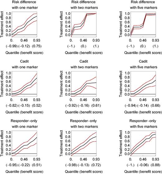
The subpopulation treatment effect pattern plot (STEPP) applied to hypothetical data for three benefit functions with one, two, or five markers. Dashed lines denote 95% confidence intervals. The horizontal axis is the quantile of the benefit score (with the benefit score in parentheses ). The vertical axis is the treatment effect measured as a difference in the probability of a binary outcome. The optimal cutpoint occurs where the lower bound of the confidence interval crosses the horizontal axis.
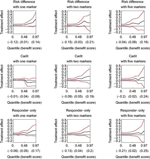
The subpopulation treatment effect pattern plot (STEPP) applied to BIG 1-98 breast cancer data for three benefit functions with one, two, or five markers. Dashed lines denote 95% confidence intervals. The horizontal axis is the quantile of the benefit score (with the benefit score in parentheses ). The vertical axis is the treatment effect measured as a difference in the probability of disease-free survival at three years. The wide confidence intervals preclude a recommendation.
The central role of DIF ( s ) in the net benefit equation motivates the risk difference benefit function, which is the difference between 1) the probability of favorable outcome given the new treatment and the markers and 2) the probability of a favorable outcome given the old treatment and the markers. To our knowledge, investigators have previously only applied STEPP with multiple markers to the risk difference benefit function ( 3 , 10 , 13 ). However, one can apply STEPP with multiple markers to other benefit functions.
As we show in the Supplementary Materials (available online), the risk difference benefit function has the desirable property that ordering test sample participants by their risk difference benefit scores orders them by the predicted net benefit of marker-based treatment selection. Two other benefit functions, cadit and responders-only, share the same desirable property because they are monotonically increasing functions of the risk difference benefit function. The cadit benefit function ( 14–16 ) is the probability that cadit equals 1 given the markers, where cadit equals 1 if the outcome is favorable under the new treatment or unfavorable under the old treatment, and 0 otherwise. The responders-only benefit function is the probability of having been assigned to the new treatment randomization group given the markers and a favorable outcome (hence a responder); it extends previous responder-only formulations involving a single binary marker ( 17 , 18 ).
STEPP Example
We discuss the computation of STEPP for multiple markers using data from the BIG 1-98 randomized trial ( 2 ) that compared tamoxifen (old treatment) vs letrozole (new treatment) for treating breast cancer ( 19–22 ). The candidate markers x were percent of immunostained cells with estrogen receptor, percent with progesterone receptor, percent with KI-67, tumor size, number of positive nodes, age at enrollment, and body mass index. To investigate the three benefit functions, we created a binary outcome Y = 1 if disease-free survival at three years, and 0 otherwise. Removing the 33 participants with missing marker data and the 18 participants censored before three years yielded 1529 patients in the tamoxifen group and 1500 in the letrozole group. For the overall analysis, there was an increase in disease-free survival of 0.935–0.906 = 0.029 (95% confidence interval = 0.010 to 0.048).
For the training sample, we fit the appropriate stepwise logistic regressions. On each step, the stepwise logistic regression adds the marker that most improves the classification of participants as Y = 0 or Y = 1. We used the area under the receiver operating curve (AUC) as measure of classification performance. Because it is difficult to select a threshold change in AUC to determine when to stop adding markers to the logistic regression, we opted instead for a sensitivity analysis, fixing the number of markers in the stepwise regression as one, two, and five. Theoretical and empirical results have shown that the marginal gain in classification performance is usually small after about five markers are included in a prediction model ( 23–25 ).


For each participant in the test sample, we substituted the markers x into the benefit function to compute a benefit score. Each test sample participant contributes a triplet (benefit score, outcome, randomization group) to the computation of STEPP. For example, consider a hypothetical test sample participant with x* = {2 positive nodes , 10 percent with KI-67 }. Substituting x * into equation (2), the risk difference benefit score for this participant is expit {4.24 – 0.433 × 2} – expit {2.98 – 0.044 × 10} = 0.04. Suppose this hypothetical participant has outcome Y = 1 and was assigned letrozole. This person contributes the triplet (0.04, Y = 1, letrozole) to the computation of STEPP.
For all the test sample participants, we create a list of the aforementioned triplets, ordered from smallest to largest benefit score. For illustration, suppose the test sample consists of 10 participants with the following ordered triplets: (0.01, Y = 0, tamoxifen), (0.04, Y = 1, letrozole), (0.12, Y = 0, tamoxifen), (0.14, Y = 0, letrozole), (0.15, Y = 1, letrozole}, (0.17, Y = 0, tamoxifen), (0.23, Y = 1, letrozole), (0.25, Y = 0, letrozole), (0.26, Y = 1, tamoxifen), (0.27, Y = 1, letrozole). For participants with benefit scores greater than cutpoint s = 0.11, there are three favorable outcomes of Y = 1 among the five participants assigned to letrozole and one favorable outcome among the three participants assigned to tamoxifen. This gives DIF (0.11) = 3/5 – 1/3 = 0.27. The smallest benefit score greater than the cutpoint 0.11 is 0.12, which is the third smallest out of 10 benefit scores and thus corresponds to a quantile of 0.30. Repeating this calculation for various cutpoints gives the entire STEPP. We computed simultaneous 95% confidence intervals for STEPP by resampling the data at the selected cutpoints to compute an appropriate multiplier of the standard error.
Extension to High-Dimensional Data
High dimensional data refers to the presence of many markers (sometimes hundreds or thousands), as often arises from high-throughput biological assays. The presence of high-dimensional data does not substantially affect the computation of STEPP in the test sample but does substantially affect model fitting in the training sample. It is computationally slow to apply the stepwise logistic regressions when a large number of markers are candidates for inclusion in the stepwise logistic regression. Therefore, with high-dimensional data, a commonly used first step is to select a relatively small preliminary set of candidate markers (numbering perhaps 20) for possible inclusion in the stepwise logistic regression. A simple measure of the predictive value of an individual marker is the absolute value of the difference in mean values between those with a favorable outcome ( Y = 1) and those with an unfavorable outcome ( Y = 0), divided by the standard error of this difference.
Extension to Survival Data
We have focused on a binary outcome because it was the basis of the decision analysis and the three benefit functions apply to binary outcomes. For survival outcomes, we discuss an extension of the risk difference benefit function.
For the computation of STEPP in the test sample, the extension to survival data is straightforward. For each participant, we compute the quadruplet (benefit score, survival time, censoring or failure indicator, randomization group). Using the quadruplets from all test sample participants, we compute DIF ( s ) as a difference in Kaplan-Meier estimates for a prespecified time. To avoid specifying a prespecified time in a survival analysis, some statisticians summarize survival data using a hazard ratio in a proportional hazards model. However, the proportional hazards assumption may not hold. More importantly, many clinicians find summary measures based on differences as clinically more informative than summary measures based on ratios ( 26–29 ).
The main computational challenge with extending STEPP to survival data is fitting a flexible stepwise parametric model that allows for censored survival data. In the Supplementary Materials (available online), we discuss a novel flexible parametric model for survival data for each randomization group that focuses on the same prespecified time used in the test sample. For each participant, we generate an outcome of 1 if death occurs before the prespecified time, 0 if survival occurs before the prespecified time, and the Kaplan-Meier estimated survival to the prespecified time conditional on censoring time, if censoring occurs before the prespecified time. Using this outcome, we apply a stepwise logistic regression that allows for fractional outcomes.
Results
Hypothetical Data
To investigate the methodology, we created hypothetical data from a trial with 600 persons in each randomization group and a binary outcome. As discussed in the Supplementary Materials (available online), we randomly generated 100 independent marker values for each participant. We next randomly generated a binary outcome for each participant using a risk difference function with two different pairs of markers for each randomization group. We randomly split the data in training and test samples, so that the data in both samples follow the same distribution.
Figure 1 shows STEPP for these hypothetical data under the three benefit functions, each with one, two, and five markers. The farther left the optimal cutpoint (where the lower bound of STEPP crosses the horizontal axis for H = 0), the better the STEPP because the beneficial subgroup has more participants. The STEPPs for the three benefit functions are similar, all with excellent performance, giving optimal cutpoints far to the left. Given that one marker in each randomization group was most predictive in the data generation, it is not surprising that all three benefit functions performed well for one marker. The exceptional performance of the risk difference benefit function with two markers per randomization group is not surprising given that it corresponds to the benefit function for data generation. If these data were real, we would conclude that a subgroup of participants created from benefit scores larger than the optimal cutpoint would have sufficiently large treatment effect to warrant a confirmatory study.
BIG 1-98 Randomized Trial
Figure 2 shows STEPP for data from the BIG 1-98 breast cancer randomized trial of tamoxifen vs letrozole under the three benefit functions with the three fixed numbers of markers. With one marker, the cadit benefit function performed noticeably worse than the risk difference and responders-only benefit functions. For two or five markers, the three benefit functions performed similarly. For all three benefit functions at all three levels of markers, the lower bounds of the 95% confidence intervals were near or below zero; there was no clear crossing of the lower bound of STEPP across the horizontal axis, as with the STEPP for the hypothetical data. We conclude there is insufficient evidence that a subgroup of participants created from our benefit scores has a sufficiently large treatment effect to warrant further study.
Discussion
The three benefit functions differ in the number of parameters and the number of participants used to the fit the model. Although these characteristics affect the performance of STEPP, our examples suggest that the most important determinant of STEPP performance is the number of markers in the model. Hence, the sensitivity analysis with one, two, and five markers is important. In choosing the benefit function, investigators should primarily consider the type of trial and the type of outcome.
For a cancer prevention trial, investigators should use a responder-only benefit function. The outcome of a cancer prevention trial is typically cancer incidence or mortality after a long time period of follow-up. Because these outcomes are rare, investigators can substantially reduce costs by collecting specimens and testing for markers only from responders in the training sample. With the test sample, investigators need specimens from all participants but need only test for those markers identified by stepwise fitting algorithm in the training sample.
For cancer treatment trials with survival endpoints, investigators should use a risk difference benefit function because it extends most readily to survival data. For cancer treatment trials with binary outcomes, investigators could consider all three benefit functions. Nevertheless, if two benefit functions involve the same set of markers and similar performance but one has fewer parameters, the one with fewer parameters is preferable to reduce the chance of overfitting.
In terms of the width of the confidence intervals for STEPP, the main determinant is the size of the test sample. Because the benefit function is fixed for test sample evaluation, any variability in the fitting of the benefit function does not affect the width of the confidence interval.
The major limitation with STEPP for multiple markers is its inability to detect small treatment effects in a subgroup because of the small sample size. The 50%-50% split into training and test samples halves the sample size for evaluation. The subgroup with the highest benefit score may further reduce sample size to 10% or less. Nevertheless, if specimen collection and marker testing is feasible, it is worthwhile to apply STEPP with multiple markers on the chance that there is a large, statistically significant treatment effect. Software written in Mathematica ( 30 ) for both binary and survival outcomes is available at http://prevention.cancer.gov/research-groups/biometry/staff/stuart-g-baker-scd .
Funding
This research was supported by the National Institutes of Health.
Notes
The authors thank the International Breast Cancer Study Group for providing the data from the BIG 1-98 trial. The statements contained herein are solely those of the authors and do not represent or imply concurrence or endorsement by the National Institutes of Health. The study sponsor had no role in the design of the study; the collection, analysis, or interpretation of the data; the writing of the manuscript; or the decision to submit the manuscript for publication.
References
References

