


Abstract
The reintroduced population of Mexican gray wolves (Canis lupus baileyi) continues to rely on a carefully managed captive breeding program. Although success of that program depends on detailed knowledge of reproductive processes, age of puberty has not been determined. This study assessed male puberty status (presence of sperm in ejaculates), maintained in nine US facilities, during their first breeding season. Variables possibly associated with puberty were also evaluated. There was a significant effect of body weight, testis size, facility latitude, and date of collection, whereas a statistical trend was found for age and inbreeding coefficient. Social factors, including being housed with sire, had no effect. Over half the males in their first breeding season were producing sperm, although in some cases sperm quality was poor, suggesting possible infertility. Although there was no minimum body weight associated with presence of sperm, likelihood increased with increasing body weight, highlighting a possible critical role for nutrition. The trend for sperm production in males collected later in the breeding season and at lower latitudes suggests that later collections, especially at higher latitudes, might reveal a higher percentage of pubertal males. These results have potential implications for breeding program management and introduce the possibility that more wild gray wolves than previously thought might produce sperm during their first year, even if they do not sire young.
La población reintroducida de lobo mexicano (Canis lupus baileyi) depende aún de un programa de reproducción en cautiverio cuidadosamente gestionado. Aunque el éxito del programa depende del conocimiento detallado de los procesos reproductivos, la edad de la pubertad no ha sido determinada. Este estudio evaluó el estado de pubertad de los machos (presencia de espermatozoides en los eyaculados) mantenidos en nueve instituciones de los Estado Unidos, durante su primera temporada reproductiva. También se evaluaron variables asociadas posiblemente con la pubertad. Se encontró un efecto significativo del peso corporal, el tamaño de los testículos, la latitud de la institución y la fecha de recolección; mientras que para la edad y el coeficiente de consanguinidad se encontró una tendencia estadística. Factores sociales, incluyendo estar alojado con el padre, no tuvieron ningún efecto. Más de la mitad de los machos en su primera temporada reproductiva produjeron espermatozoides, aunque en algunos casos la calidad era deficiente, lo que sugiere una posible infertilidad. Aunque no hubo un peso corporal mínimo asociado con la presencia de espermatozoides, la probabilidad aumentó con el aumento del peso corporal, destacando el posible papel crítico de la nutrición. La tendencia de producción de espermatozoides en los machos recolectados en fechas posteriores en la temporada de reproducción y en latitudes más bajas, sugiere que recolecciones más tardías, especialmente en latitudes más altas, podrían revelar un mayor porcentaje de machos púberes. Estos resultados tienen implicaciones potenciales en la gestión del programa de reproducción e abren la posibilidad de que más lobos grises silvestres puedan producir espermatozoides durante su primer año de lo que se pensaba anteriormente, incluso si no producen crías.
Mexican gray wolves (Canis lupus baileyi), a subspecies of the Gray Wolf (C. lupus) once widespread across the Southwestern United States and northwestern Mexico, were considered extinct in the wild after about 1980. However, after certification as Mexican gray wolves (Hedrick et al. 1997), three lineages of captive wolves, with a total of seven individual founders, were incorporated into a binational breeding program in US and Mexican zoos in the late 1990s. Descendants from that breeding program were first reintroduced into Arizona and New Mexico in 1998 (Parsons 1998) and into Mexico in 2011 (Araiza et al. 2012). The free-ranging populations still depend on and benefit from exchanges with the captive population, with problem wolves being brought back into captivity and captive wolves being released or pups cross-fostered. Thus, successful management of captive Mexican wolves remains essential for the free-ranging population to thrive.
There are currently 387 Mexican wolves in 62 US and Mexican zoos (Mexican Wolf Population Analysis and Breeding and Transfer Plan 2022; Scott et al. 2022). Each year recommendations for breeding pairs are generated using the software program PMx (Ballou et al. 2022a) from data in the Mexican Gray Wolf Studbook (Greely 2021), a computer-based pedigree, to minimize inbreeding and maximize founder representation and genetic heterozygosity of the population. Wolves not receiving a breeding recommendation must be separated from opposite-sex wolves, treated with a contraceptive, or, if aged, may be permanently sterilized.
Wolves typically mate monogamously, but their social organization can extend beyond the male–female pair to include young of the year and of previous years. Although several variations of their mating system and social organization have been documented (Mech and Boitani 2003), especially in Yellowstone National Park (Stahler et al. 2013), those variations may be an exception, resulting from the highest known densities of both wolves and their prey (Mech and Barber-Meyer 2015).
Zoos prefer to maintain species as naturally as possible, so in the case of wolves, this can mean that offspring of various ages may be housed with their parents. Thus, if the parents receive a breeding recommendation, concern remains about possible mating attempts involving young wolves in the group. Although Gray Wolf parents have been reported to prevent their offspring from mating while they remain in the pack (e.g., Rabb et al. 1967; Packard and Mech 1980), the critical importance of avoiding inbreeding among Mexican wolves necessitates ensuring that those young wolves are not allowed to reproduce. However, welfare considerations favor keeping them within the family social unit, so it is imperative to know at what age they become fertile.
Documentation of puberty in free-ranging populations is typically based on birth of offspring, also called age of first reproduction, but that does not necessarily represent when they first become fertile. Many factors other than fertility affect successful reproduction, in particular, social maturity. Even age of first reproduction can be difficult to document for males unless parentage of offspring can be confirmed. Age of first possible reproduction for female gray wolves has been reported to be two years of age (Murie 1944; Rausch 1967; Peterson et al. 1984; Fuller 1989), with the assumption that it is the same for males. Most exceptions have been found in captive wolves (Lentfer and Sanders 1973; Medjo and Mech 1976), possibly explained by artifacts of captivity, such as altered social units or enhanced nutrition. However, a recent study of free-ranging gray wolves in Sweden and Norway found that 1% of males reproduced at one year of age (Wikenros et al. 2021), although possible explanations for the earlier puberty in those males were inconclusive.
Other than production of offspring, there are multiple possible indicators of puberty in males, such as appearance of secondary sex characteristics, reaching a critical body weight or condition threshold, and increase in size of testes (Gobello 2014). There are no clear secondary sex characteristics in wolves, and thresholds of body weight or testis size have not been established. A definitive marker of sexual maturity is production of sperm (e.g., domestic dogs; Johnston et al. 2001). Although presence of sperm can be challenging to assess in free-ranging wolves, it is rather straightforward in captive individuals.
In 1990 our team was given the responsibility for annual collection and cryopreservation of semen from candidate males by the US Fish and Wildlife Service Mexican gray wolf recovery team (see Ballou et al. 2022b). For this study, we used the opportunity of that annual project to evaluate the fertility of young male Mexican wolves during their first breeding season via standard semen collection methods. In addition, to better understand social factors that might influence the timing of puberty, we noted the composition of the social units of young males and, as possible external indicators or predictors of puberty, we measured testis size and body weight. Latitude can affect onset of breeding season in gray wolves (Mech 2002), with more northerly populations breeding later than those further south. Because it might also affect onset of puberty, we included latitude of the participating facilities in analyses.
Materials and Methods
Animals.
The 57 wolves used in the study, ranging in age from eight months 17 days to 10 months 18 days, were housed at nine facilities in the United States (Table 1). Because all Mexican wolves are part of the binational recovery program, husbandry practices follow strict guidelines that are similar across all institutions, reducing that source of variability. However, the cooperating institutions included urban zoos, rural wolf breeding centers, and remote Mexican wolf prerelease facilities (Table 1), so extent of exposure to humans and human-generated disturbance varied across institutions. In addition to the relative differences in density of local housing and traffic, urban zoos are open to the public, but rural wolf breeding centers are only open by appointment for tours and for educational programs, limiting exposure to human visitors---prerelease facilities are not open to the public.
Locations where study males were housed, categorized by whether the facility was situated in an urban, rural, or remote area.
| Institution | Location | Number of males |
|---|---|---|
| Urban: | 10 | |
| Brookfield Zoo | Brookfield, Illinois | 4 |
| Phoenix Zoo | Phoenix, Arizona | 3 |
| ABQ BioPark | Albuquerque, New Mexico | 1 |
| Sedgewick County Zoo | Wichita, Kansas | 2 |
| Rural: | 44 | |
| California Wolf Center | Julian, California | 15 |
| Endangered Wolf Center | Eureka, Missouri | 18 |
| Wolf Conservation Center | S. Salem, New York | 11 |
| Remote: | 3 | |
| Ladder Ranch | Caballo, New Mexico | 2 |
| Sevilleta National Wildlife Refuge | La Joya, New Mexico | 1 |
Six males were born in the wild in Arizona or New Mexico and cross-fostered into captive packs between estimated 10 and 14 days of age. All others were born into captive packs and remained with at least some members of their natal pack at the time of collection.
All animal handling followed ASM guidelines (Sikes et al. 2016). Procedures fell within and were the same as IACUC protocols approved for wolf semen collection and banking for the years of the study.
Sample and data collection and analyses.
Samples were collected each year between 23 January and 9 March during five breeding seasons (2017–2021). Procedures were carried out with wolves under general anesthesia; the drug regimen varied slightly among institutions, depending on the preference of local attending veterinarians. Because some anesthetics can interfere with semen collection, options were restricted to Telazol (tiletamine plus zolazepam) or ketamine plus either midazolam or diazepam; isoflurane was often used to maintain anesthesia after induction. Before stimulation for semen collection, testes were measured (length, width, and depth) using calipers, and combined testes volume was calculated using the formula for an ellipsoid (W × D × L × 0.524 cm).
To minimize urine contamination of semen samples, the urinary bladder was flushed with sterile saline. Semen was collected by electroejaculation (Model 12 electroejaculator; G & S Instruments, Midlothian, Texas) using a 3-cm-diameter probe with three linear electrodes (PT Electronics, Boring, Oregon) placed ventrally in the rectum. Stimulation was slowly increased until the hind limbs extended, returned to zero, and repeated rhythmically, with an approximately 5-s cycle, at gradually increasing voltages until fluid was obtained. Because depth of anesthesia can dampen neural response, adequate stimulation was judged by extent of hind-limb extension. Amperage (a measure of electrical current and indication of circuit completion), rather than voltage (a measure of electrical stimulus generation) was monitored. To prevent rectal overheating, current was limited to ≤300 mAmps.
Samples were examined immediately under phase-contrast microscopy at 200× for presence of sperm; in samples with sperm, percent motile sperm was estimated. Sperm morphology was assessed at 400× after eosin–nigrosin staining. For concentration, a sample aliquot was diluted with acetic acid to immobilize sperm, which were then quantified using a Makler Counting Chamber (Sefi-Medical Instruments, Haifa, Israel). Concentrations of samples with very small volumes were quantified by counting the number of sperm cells in a drop of semen examined in a 200× microscope field. The percentages of motile and morphologically normal sperm were used to estimate the potential fertility of samples (adapted from Oettlé 1993): fertile (both values ≥ 60%); subfertile (one value 40–59% and the other ≥60% or both 40–59%); and infertile (both values ≤ 39%). Information on animal birth dates, body weights, and social units was provided by staff at participating institutions. Inbreeding coefficients (F) were calculated by the additive matrix method (Ballou 1983), using the pedigree of the Mexican wolf captive population. For any wolves (other than original founders) with unknown or uncertain parentage, the additive matrix method was extended, as described in Lacy (2012).
Statistics.
Variables describing males with and without sperm were compared using multivariate analysis of variance (MANOVA; NCSS, Kaysville, Utah), including age in days, collection date (representing point in breeding season), latitude, testis volume, and inbreeding coefficient. Body weight was separately evaluated using a two-sample T-test, due to missing values for six males, precluding that parameter from the MANOVA. Relationships between parameters were assessed by Pearson product-moment correlation (NCSS). Kaplan–Meier Survival Analysis (Systat, Palo Alto, California) was used to further analyze the parameters of age, body weight, and testis volume. The alpha level for statistical significance was set at 0.05 for all tests.
Results
Sperm were detected in semen samples from 31 of the 57 young males (54.4%). The ages of males with and without sperm did not differ significantly, but there was a trend for those with sperm to be older (Table 2, Fig. 1). Nevertheless, even one of the youngest (eight months 17 days) had sperm. Body weight was significantly greater in males with sperm (Table 2; Fig. 1). Body weight maximums were similar in the two groups (36.1 kg for males with no sperm and 37.2 kg for those with sperm), but none of the males below 22.4 kg were producing sperm at the time of collection. Despite the trend for sperm production in older and larger males, age and body weight were not correlated (P = 0.22, r = 1.18).
Comparison of multivariate analysis of variance (MANOVA) results between males with and without sperm in samples.
| Variablea | n | Mean | SE | Min | Max | Median | P | F |
|---|---|---|---|---|---|---|---|---|
| Age-N | 25 | 282.8 days (9 months 8 days) | 3.5 | 262 days (8 months 17 days) | 325 days (10 months 19 days) | 283 days (9 months 8 days) | 0.061 | 3.65 |
| Age-Y | 31 | 290.2 days (9 months 14 days) | 2.2 | 262 days (8 months 17 days) | 325 days (10 months 19 days) | 291 days (9 months 15 days) | ||
| Testes-N | 25 | 15.5 cm3 | 1.3 | 3.4 cm3 | 29.0 cm3 | 15.2 cm3 | 0.00001b | 23.14 |
| Testes-Y | 31 | 24.8 cm3 | 1.4 | 14.0 cm3 | 40.9 cm3 | 23.8 cm3 | ||
| Collection date-Nc | 25 | 39.7 days | 2.1 | 23 days | 68 days | 39 days | 0.002b | 10.84 |
| Collection date-Yc | 31 | 48.1 days | 1.8 | 29 days | 68 days | 51 days | ||
| Inbreed-Nd | 25 | 0.16 | 0.017 | 0.12 | 0.42 | 0.14 | 0.094 | 2.91 |
| Inbreed-Yd | 31 | 0.14 | 0.001 | 0.12 | 0.16 | 0.14 | ||
| Collection latitude-N | 25 | 38.06°N | 0.63 | 33.01°N | 41.49°N | 38.31°N | 0.04b | 5.32 |
| Collection latitude-Y | 31 | 36.28°N | 0.58 | 33.02°N | 41.49°N | 37.43°N | ||
| BW-N | 24 | 27.6 kg | 0.98 | 15.2 kg | 36.1 kg | 27.85 kg | 0.013b | 2.59e |
| BW-Y | 25 | 30.8 kg | 0.77 | 22.4 kg | 37.2 kg | 31.2 kg |
aY = yes sperm in sample; N = no sperm in sample.
bSignificant difference between males with and without sperm in the samples collected.
cJulian date for the year semen sample was collected.
dInbreeding coefficient (F).
eValue of T from T-test, rather than MANOVA, due to missing body weight data for some males.
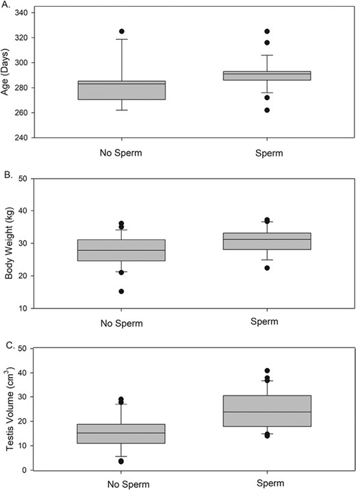
Comparison of males with and without sperm in their samples on the variables (A) age in months and days at time of collection, (B) body weight, and (C) combined testis volume.
Combined testis volume was significantly greater in males producing sperm, with especially small volumes in some of the males not producing sperm (Table 2, Fig. 1). Furthermore, testis volume showed a strong, significant correlation with body weight (P < 0.0001, r = 0.61), but testis volume was not correlated with age (P = 0.22, r = 0.18). Kaplan–Meier analysis showed the 25%, 50%, and 75% likelihood of sperm production for each of these parameters (Table 3).
Percentage likelihood that a male will have sperm in a sample for the variables age, body weight, and testis volume.
| % of males with sperm | Age at collection | Body weight (kg) | Testis volume (cm3) |
|---|---|---|---|
| 75% | 10 months | 36 | 35.3 |
| 50% | 9 months 15 days | 31.9 | 23.2 |
| 25% | 9 months 11 days | 30.3 | 20.9 |
| % of males with sperm | Age at collection | Body weight (kg) | Testis volume (cm3) |
|---|---|---|---|
| 75% | 10 months | 36 | 35.3 |
| 50% | 9 months 15 days | 31.9 | 23.2 |
| 25% | 9 months 11 days | 30.3 | 20.9 |
Sample collection date (expressed as Julian date beginning 1 January for the year of collection) also had a significant influence, with sperm more likely found in samples collected later in the breeding season (P = 0.002, F = 10.84). Similarly, wolves living at lower latitudes were more likely to be producing sperm (P = 0.04, F = 5.32; Table 2, Fig. 2). Inbreeding coefficients were not different between the two groups (P = 0.09, F = 2.91; Table 2, Fig. 2), although the two males with the highest inbreeding coefficients (0.4152) had no sperm.

Comparison of males with and without sperm in their samples on the variables (A) sample collection date (Julian date), (B) collection latitude (degrees), and (C) inbreeding coefficient.
Of the samples containing sperm, motility ranged from 0 to 90% and normal morphology from 0 to 94%. However, based on percentages of motile and normal sperm, many of the samples fell within the categories of subfertile or infertile (Table 4). Only 7 (22.6%) of the 31 males would be considered fully fertile, with both percent motility and normal morphology of ≥ 60%, whereas 8 (25.8%) would be classified as infertile, with both of those values ≤ 30%. Sample concentration varied considerably, ranging from a high of 166.6 × 10⁶/ml to amounts too low for an accurate count (n = 17).
Percentages of morphologically normal or motile sperm characterizing fertility categories of sperm samples.
| Estimated fertility categories | Range of % normal or % motile sperm in each fertility category | % samples with motility within each fertility category | % samples with normal morphology within each fertility category (n) |
|---|---|---|---|
| Fertile | ≥ 60% | 41.9% (13) | 25.8% (8) |
| Subfertile | 40–59% | 16.1% (5) | 19.4% (6) |
| Infertile | ≤ 39% | 41.9% (13) | 29.0% (9) |
| Undetermined | Too few sperm to assess | NA | 25.8% (8) |
Social unit composition appeared not to determine whether a male was producing sperm. No male was separated from his sire or foster sire, and yet more than half had sperm. A similar number of those with (four) and without sperm (five) were separated from their dams. For young males living in their natal groups that also contained male and/or female littermates, 58% had sperm and 42% did not. When male littermates were present, one or more brothers might have sperm while other brothers did not, but dominance rank among male littermates was not assessed.
Most wolves sampled were at wolf centers in rural settings (n = 44); of those 23 were producing sperm and 21 were not. Of the 10 at urban zoos, eight males had sperm and two did not. However, none of the samples from the three males at the remote, prerelease facilities contained sperm. Two of those were among the youngest sampled (8 months 17 days), were brothers that had been transferred from the other remote facility, and were collected early in the breeding season (8 February); their inbreeding coefficients (0.1461) were near the median. Both facilities are located in the lower range of latitudes of those included in the study.
Nine males were not at their natal location when sampled. Six wild-born males had been removed from their natal dens and cross-fostered to captive female wolves, and three captive-born males had been moved with their respective natal groups to another facility. Only one of the six wild-born, cross-fostered males was producing sperm. His testis volume was relatively large but the other variables fell within the range of the five without sperm. All wild-born, cross-fostered males had relatively high inbreeding coefficients (0.2509–0.4152); at the time of collection one was housed at an urban zoo and the other two at rural wolf centers. Of the three males transferred, along with their families, from their natal locations to the facilities where semen was collected, one had sperm. The two without sperm were the same brothers mentioned above that had been moved from one remote facility to the other.
One male had undescended testes. He was 9 months 15 days of age, weighed 33.2 kg, was sampled mid-season on 24 February, and had a mid-range inbreeding coefficient of 0.1564. He was still living at his natal location, a rural wolf center, and housed in his natal group.
Discussion
Although gray wolves, including the Mexican gray wolf subspecies, have long been thought to reach puberty in their second year, 54.4% of the males in this study were producing sperm during their first breeding season. However, not all males with sperm in their samples were judged to be fertile. Many semen samples were of poor quality, with only 22.6% of all sampled males judged to be fully fertile, based on assessments of sperm motility and normal morphology both being ≥ 60%. However, the males judged to be subfertile (the intermediate category with one or both those parameters being between 40 and 59%) might still achieve fertilization via multiple matings. Data from domestic dogs have shown that multiple inseminations can result in pregnancy even when sperm quality is poor (Mickelsen et al. 1993). The wolf estrous period has been reported to be nine–15 days (Kreeger 2003), during which mating may take place multiple times per day. The implications for Mexican wolf management are that most if not all young males producing sperm might achieve fertilization if housed with females during the breeding season.
There was a trend for age to be associated with sperm production, with median age for those with sperm being one week older. However, there was complete overlap in the age range, with the same minimum and maximum ages for both groups. Even one of the youngest (8 months 17 days) had sperm, so age was not a limiting factor in the range represented in this study. The probability of sperm production did increase with increasing age, but age also increases as the breeding season progresses, and more males collected later in the season were producing sperm.
Body weight was significantly greater for males with sperm. No male weighing below 22.4 kg had sperm, and the probability of producing sperm increased with increasing body weight. This result is not surprising, given the general association of body weight with initiation of puberty (Frisch 1984; Baker 1985), something also reported for gray wolves (Mech 2006) and closely related coyotes, C. latrans (Sacks 2005). Although plentiful high-quality diets are provided to all captive Mexican wolves, not every individual may have had access to the same amount, due to competition among animals housed together. That, plus possible genetic differences influencing growth rates, might explain why some males reached a body condition that initiated pubertal processes while other male littermates living in the same group did not.
As expected, testis size was significantly larger for males producing sperm. Testicular volume is associated with size and activity of seminiferous tubules, the site of spermatogenesis, as well as with increased Leydig cell production of testosterone, which is needed to support spermatogenesis. Thus, size is a good indicator of testicular activity and sperm production. Testis size was correlated with body weight, as has also been reported for gray wolves (Mech 2006) and coyotes (Kennelly 2001). This observation is consistent with the hypothesis that puberty is dependent on attaining sufficient body condition to support reproduction (e.g., Frisch 1984).
Semen collection date was also associated with the presence of sperm, with detection of sperm becoming more likely later in the breeding season. Of the five males collected in late January in this study, only one was producing sperm. However, our experience of successfully collecting and banking semen from Mexican wolves at these and other facilities has encompassed the period from late January through early March; fertility of males in the full population during this period is confirmed by birth dates recorded two months later (Greely 2021). It has been reported that coyotes in their first breeding season start producing sperm later than the adults in the same population (Gier 1975; Kennelly 2001). Thus, it is possible that collections later in the season might have yielded sperm in more young male Mexican wolves. In a small study of adult Mexican wolves, we detected sperm (although of relatively low quality and quantity) in two of six males as early as October and in all by January (Asa C.S., Bauman K.L., St. Louis Zoo, personal observations). These results suggest that even as early as January, we might expect to see at least some sperm cells in samples of males reaching puberty that breeding season, but with higher likelihood later in the season in young males.
Another factor associated with presence of sperm was latitude of the facility. Males at lower latitudes were more likely to be producing sperm at the time of collection, a finding that agrees with the report that breeding season is earlier in gray wolves at lower latitudes (Mech 2002). The proportion of males producing sperm was similar in urban zoos and rural wolf centers, but none of the three young males at the remote, prerelease facilities had sperm at the time of semen collection. These facilities are in the lower range of latitudes of those in the study, which should favor earlier sperm production. Factors that may have reduced likelihood of spermatogenesis in two of those males included transfer from natal location, being among the youngest, and being sampled early in the season.
The difference in inbreeding coefficients between males with and without sperm was not significant but showed a trend (P = 0.09) for lower inbreeding to be associated with presence of sperm. In support of that trend, neither of the two males with the highest inbreeding coefficient (0.4152) and only one of three with the next highest (0.2800) had sperm. Furthermore, fertility may be in question even for highly inbred males with sperm, since our earlier analysis showed that inbreeding can affect sperm quality, especially morphology (Asa et al. 2007). In this study, the most highly inbred male with sperm did have low-quality sperm (30% motile, 0% normal morphology) and was considered infertile.
Only two of nine males that had been transferred from their natal locations were producing sperm: one wild-born, cross-fostered and one captive-born moved with its natal group. Although the numbers are small, outcomes suggest that being moved during the first year may affect timing of puberty. However, another factor common to the cross-fostered males was high inbreeding coefficients (> 0.2500), which may have contributed to slower reproductive development. Regarding other parameters, cross-fostered males without sperm were sampled both early and late in the season, and their ages were both above and below the means, whereas their body weights were all at or below the group mean for other males without sperm. Their smaller body size is another indicator that they may have been developing more slowly.
Group composition did not determine whether a male was producing sperm. No males were separated from their sires or foster sires, demonstrating that males can reach puberty even when living with their sires or another adult male. Our results are consistent with observations in gray wolves that subordinates are prevented from reproducing by behavioral interference rather than physiological suppression (Packard et al. 1983). It would be interesting, however, to know whether spermatogenesis rates might be even higher in males separated from sires and thus removed from potential dominance-related suppressive effects.
Of the nine males separated from their dams, almost half had sperm, which approximates the overall percentage of males with sperm. Similarly, some males had sperm and some did not in groups that contained male and/or female littermates. However, because some litters contained brothers with and without sperm, it will be important to determine in future studies whether relative dominance rank among male littermates might affect which brothers reach puberty during their first year. For example, dominance rank may influence access to food, which can affect growth rate, or stress responses, which can affect fertility (e.g., Giblin et al. 1988).
In summary, in this study greater body weight was the best predictor that a male Mexican wolf would reach puberty, judged by production of sperm, during his first breeding season. The availability of abundant, high-quality food to captive animals may provide a nutritional plane fueling more rapid growth. Sperm production has not been assessed in wild populations of wolves, with those studies relying instead on siring pups as an indicator of reproductive maturity. However, it is possible that even in free-ranging populations, more young male wolves than previously thought may be producing sperm during their first breeding season. Ecological and social factors may be more important than reproductive maturity in influencing whether a young male disperses or remains in his natal group. That is, reproductive maturity is necessary but not sufficient for production of young. There has been no reported measurement of testosterone levels of dispersing versus nondispersing young male wolves, but it is generally believed that dispersal is associated with testosterone elevation during puberty—for example, Spotted Hyena, Crocuta crocuta (Holekamp and Smale 1998) and Chacma Baboon, Papio ursinus (Beehner et al. 2006). This raises the question of whether young male wolves that disperse before one year of age might be producing sufficient testosterone to support spermatogenesis, even if they fail to produce pups that season. The implication for the Mexican wolf captive breeding program is that as many as half of young males may produce sperm during their first breeding season. However, not all may be fully fertile and their sires may prevent them from mating. Nevertheless, social management should take their potential fertility into account.
Acknowledgments
The authors thank all the participating institutions, A. Franklin for assistance with statistical analysis, P. Maciel-Cabanas for Spanish translation of the abstract, L. D. Mech for summarizing current thinking on the gray wolf mating system, and R. Lacy for explanation of inbreeding coefficient calculation.
Conflict of Interest
The authors confirm that they have no conflicts of interest, financial or otherwise, to disclose.
Funding
Funding was provided by the US Fish and Wildlife Service, the AZA Mexican Wolf Species Survival Plan, and the Saint Louis Zoo.
Author Contributions
CSA conceived and designed the study, collected and analyzed samples, and wrote most of the manuscript; KLB collected some of the samples, gathered data, managed the data set, and assisted with statistical analyses and with writing the manuscript.
Data Availability
Data are available by request to the authors and with permission by the US Fish and Wildlife Service.
