Uniqueness from discrete data in an inverse spectral problem for a pencil of ordinary differential operators

Abstract

1. Introduction: new definitions and problem statements

We now describe the domain of the pencil |$L-\lambda P$|⁠. It turns out that, in some cases, the natural choice of domain is |$\lambda $|-dependent, and we require the following definition.  

The definition of the domain of the pencil |$L-\lambda P$| is slightly simplified by noting that, except when the problem is in PLP for all |$\lambda $|⁠, the point |$\lambda = 0$| always lies in the domain |$\Omega _c$| in which the equation is in PLC: see Figure C.1. Thus, in the PLC case, we can take |$U$| to be any non-trivial real-valued solution of the equation |$\ell U=0$|⁠, and use it to define a boundary condition in the usual way for the classical limit-circle case. Let |$[\cdot ,\cdot ]$| denote the Wronskian.  

To introduce the Weyl–Titchmarsh function|$m(\lambda )$| for our pencil, we first remark that, owing to the asymptotics in Appendix C, equation (1.3) has at least one non-trivial solution in |$H$|⁠. We can therefore make the following definition.  

Using the variation-of-parameters formula, one may show that, with the domains as in Definition 1.3, the operator |$L-\lambda P$| is invertible when |$m(\lambda )$| is analytic, and that the eigenvalues of the pencil |$L-\lambda P$|⁠, which are poles of |$(L-\lambda P)^{-1}$|⁠, are the poles of |$m(\lambda )$|⁠. Note that, in the case |$\nu =2,$| there is generally a discontinuity of |$m$| across the boundary curve between |$\Omega _p$| and |$\Omega _c$|⁠, due to the freedom in choosing the boundary condition function |$U$| for |${\rm Im}(\sqrt {\lambda })<1$|⁠.

The main objective of this paper is to obtain a pair of uniqueness theorems for the following.  

Our approach is firstly to show that, in both the PLP and PLC cases, the |$m$|-function is uniquely determined by its values at |$-n^2~(n\in \mathbb {N})$|⁠, then secondly to invoke the Borg–Marčenko-type theorem in Appendix A that uniquely determines a potential from its associated |$m$|-function. In the PLP case |$\nu \geq 2$| (note |$\nu =2$| turns out to be treatable by a PLP technique), we will transform (1.3) to Liouville normal form on the half-line |$[0,\infty )$|⁠, in PLP at |$\infty $|⁠, regular at 0, before utilizing the Rybkin–Tuan interpolation formula [24] for the classical limit-point |$m$|-function associated with such an equation. This is valid because the PLP and classical limit-point |$m$|-functions are formally the same where their domains overlap, that is, all of |$\mathbb {C}$| when |$\nu >2$| and |$\Omega _p$| when |$\nu =2$|⁠; the Rybkin–Tuan interpolation holds in this region. However, when |$0\leq \nu <2,$| the Liouville normal form of (1.3) holds on a finite interval; to our knowledge, there is no interpolation result for such a classical limit-circle problem.

To fill this gap, in Section 2 we will prove an interpolation result similar to that in [24], but which holds in a finite-interval limit-circle case. We will then argue using the same reasoning as in the PLP case that we may use the interpolation to prove our PLC uniqueness theorem. The uniqueness theorems will be stated and proved by the outlined methods in Section 3.

We will conclude the paper with an illustration of the relevance of this result in Section 4, where we explain how it proves a uniqueness theorem for the physically motivated Berry–Dennis PDE inverse problem, which involves boundary singularities and partial Cauchy data at the boundary.

2. Interpolation of a classical limit-circle |$m$|-function

We will use Theorem A.1 [24, Theorem 5] to prove our PLP uniqueness result. A drawback of the theorem is that it will not help for the PLC uniqueness, as it only applies to classical limit-point operators on the half-line. The purpose of this section is to establish an analogous result, for a particular finite-interval classical limit-circle Sturm–Liouville problem.

We shall follow a similar line of attack, and eventually implement (2.4). Unfortunately, the |$A$|-amplitude Laplace transform representation in [14] is not valid in the classical limit-circle case at one endpoint of a finite interval, since one cannot transform such a problem to the half-line whilst retaining the Liouville normal form. Another approach must be used.

We will find a Laplace transform representation of |$m_{h,H}(\lambda )$| by showing that its so-called Mittag-Leffler series expansion (see, for example, [12, Chapter 8]) is simply related to a Laplace transform. We then prove that condition (2.5) holds, implying the validity of interpolation formula (2.4).

Lemma 2.1 gives us enough to deduce a Laplace transform representation of |$m_{h,H}$|⁠, and hence our interpolation result. For the reader's convenience we state the theorem in full.  

The proof uses Lebesgue's dominated convergence theorem. We need the following lemma.  

3. Uniqueness theorems for the inverse problem

The main result of this paper is a pair of uniqueness theorems for Inverse Problem 1.1. We will state and prove these here, by means of Theorem A.1 and our interpolation result in Theorem 2.1. The uniqueness theorems are kept separate due to certain technical conditions in both being similar in representation, but fundamentally different in structure.  

4. The Berry–Dennis problem

Uniqueness for this inverse problem is immediate from Theorem 3.1, under the conditions |$q\in L^\infty _{{\rm loc}}(0,1]$| and |$q(r)=O(r^{\alpha -2})\ (r\rightarrow 0)$| for some fixed |$\alpha >0$|⁠. The uniqueness follows since, for positive |$n,$| the restrictions on |$q$| make the type (1.3) pencil, associated with each operator |$\mathcal L_n$|⁠, be in PLP at 0 (see [22]), whilst the sequences |$-\lambda _n=-n^2$| and |$m(-n^2)$| form the interpolation sequence required in Theorem 3.1. Thus we have proved the following theorem.  

The 0th term |$(1/\varepsilon ^2,m(1/\varepsilon ^2))$| is superfluous for our needs. However, we can go farther. Following Corollary 3.1, we may discard arbitrarily many of the diagonal terms of |$\Lambda $| and still retain uniqueness of |$q$|⁠.  

Appendix A. Limit-point interpolation and a Borg–Marčenko theorem

We collect here some useful theorems. The first is the interpolation result from [24] mentioned in Section 2 and applied in the proof of Theorem 3.1, whilst the second is a general Borg–Marčenko uniqueness result and a simple corollary, the latter being what we need in Section 3. We state the first in full to highlight its similarities with Theorem 2.1.  

Theorem A.2 was originally stated in a slightly weaker form (without the ray condition) by Simon in 1999 [25]; the above improvement was first published, with a shorter proof, by Gesztesy and Simon in 2000 [15]. An alternative, even shorter, limit-point proof was found by Bennewitz in 2001 [6]. All are generalizations of the original, much-celebrated uniqueness theorem proved separately in 1952 by Borg [8] and Marchenko [21]. As an immediate consequence we have the result we need in this paper.

Various asymptotics for a Bessel-type equation

In this appendix, we collect some necessary results on the large-|$n$| asymptotics of the eigenvalues and norming constants defined in Section 2, as well as a result on asymptotics of the |$m$|-function, needed in the same section.

The eigenvalues of the Bessel equation of zeroth order, with Dirichlet and Neumann boundary conditions at the left and right endpoints, respectively, of |$(0,1)$|⁠, are well-studied, and are algebraically equivalent to the positive zeros of the Bessel function |$J_1$|⁠. This information is enough to determine the eigenvalues |$\lambda _n$| for the boundary value problem (2.1), (2.2) and (2.6), asymptotically to order |$1/n$|⁠. We calculate these first for the unperturbed equation, and then use a result from [10] to move to the perturbed version.  

The next lemma provides a powerful asymptotic representation of the norming constants in Section 2. For its proof we will relate our notation to that of [10] and then utilize some results from the same paper.  

The large-imaginary-part asymptotics of |$m$|-functions is also a well-studied topic. The result we use in Section 2 is an application of the very general Theorem 4.1 of [5] to (2.1); we state it as a lemma.  

PLP and PLC behaviour; dimension of solution space

We will analyse here the dimension of the solution space of (1.3) with |$w(r)\sim r^{-\nu }$| and |$\nu \geq 0$|⁠. It will be helpful to treat the two cases |$\nu \geq 2$| and |$0\leq \nu <2$| separately, respectively, in Lemmas C.1 and C.3. The first analysis is by transforming the problem to Liouville normal form on the half-line and using known large-|$x$| asymptotics of solutions. The second follows a different approach, using asymptotic analysis and variation of parameters to build recursion formulae that can be used to construct a pair of linearly independent solutions.  

To prove this, we will use a result given by Eastham [13, Ex. 1.9.1], which, by providing asymptotic expressions for the solutions of equation (1.3), will give us the means to determine when any solution is in |$L^2(0,1;r\,{d} r)$|⁠. For convenience and completeness we state the form of this result, which provides the most generality when applied here.  

With this in mind, we proceed with the proof.  

Proof of Lemma C.1.

We write

\begin{align*} w(r) &= \frac{1}{r^\nu}(1+\varepsilon_1(r)), \\ \frac{q(r)}{w(r)} &= \varepsilon_2(r)\quad (r\in(0,1)), \end{align*}

where

\begin{equation} \varepsilon_j(r)=O(r^\alpha)\quad (r\longrightarrow 0,\ j=1,2). \end{equation}

(C.1)

By performing a Liouville–Green-type transformation, with

\begin{align} t(r) &= \int_r^1 \rho^{-\nu/2} \,{d} \rho\quad (r\in(0,1)), \notag\\ z(t) &= r(t)^{{(2-\nu)}/{4}} u(r(t))\quad (t\in(0,\infty)), \end{align}

(C.2)

we arrive at the following equation, for |$t\in (0,\infty ),$|

\begin{equation} -z''(t;\lambda)+ \underbrace{\left[(\varepsilon_1\varepsilon_2-\lambda\varepsilon_1+\varepsilon_2)(r) - \left(\frac{\nu-2}{4}\right)^2r^{\nu-2}\right](t)}_{{=:Q(t;\lambda)}} z(t;\lambda) = \lambda z(t;\lambda). \end{equation}

(C.3)

Note that if |$\nu >2,$| then we have |$t(r)=({(\nu -2)}/{2})(r^{1-\nu /2}-1)$|⁠, whereas if |$\nu =2,$| then |$t(r)=-\log (r)$|⁠. For conciseness, we will treat both cases |$\nu =2$| and |$\nu >2$| at the same time, as the only difference between them arises near the end of the reasoning, and will be highlighted clearly.

We want to apply Lemma C.2 to equation (C.3), for which we need |$Q(\cdot \,;\lambda )\in L^2(0,\infty )$|⁠. Since |$Q(\cdot \,;\lambda )\in L^\infty _{{\rm loc}}[0,\infty )$|⁠, the large-|$t$| behaviour of |$Q(t;\lambda )$| determines its square-integrability. Hence, |$Q(\cdot \,;\lambda )\in L^2(0,\infty )$| if and only if

\begin{equation} \infty >\int_0^\infty |(\varepsilon_1\varepsilon_2-\lambda\varepsilon_1+\varepsilon_2)(r(t))|^2 \,{d} t =\int_0^1 r^{-\nu/2} |(\varepsilon_1\varepsilon_2-\lambda\varepsilon_1+\varepsilon_2)(r)|^2 \,{d} r. \end{equation}

(C.4)

But this holds automatically, due to (C.1). Thus we have a pair of solutions |$z_\pm (\cdot \,;\lambda )$| for equation (C.3) given, as |$t\rightarrow \infty $|⁠, by

\[ z_\pm(t;\lambda)=\exp\left(\pm i \left\{\sqrt{\lambda}t - \frac{1}{2\sqrt{\lambda}} \int_0^t Q(\cdot\,;\lambda) \right\}\right) (1+o(1)). \]

Now, the integral in the argument of this exponential is easily calculated to be

\[ \int_{r(t)}^1 \left\{(\varepsilon_1\varepsilon_2-\lambda\varepsilon_1+\varepsilon_2)(\rho) -\left(\frac{\nu-2}{4}\right)^2\rho^{\nu-2}\right\}\rho^{-\nu/2} \,{d} \rho. \]

By (C.1), the first part of this integral is convergent to a finite limit as |$t\rightarrow \infty $|⁠. The second part is 0 if |$\nu =2$| and convergent if |$\nu >2$|⁠, since |$\nu -2-\nu /2>-1$|⁠. Thus, in fact, we have the leading-order asymptotics

\begin{equation} z_\pm(t;\lambda)\sim e^{\pm i\sqrt{\lambda}t}. \end{equation}

(C.5)

For any solution |$u(\cdot \,;\lambda )$| of equation (1.3) and its corresponding transformed solution |$z(\cdot \,;\lambda )$| of (C.3), we have |$\int _0^1 r|u(r;\lambda )|^2 \,{d} r = \int _0^\infty r(t)^2 |z(t;\lambda )|^2 \,{d} t$|⁠. But the leading-order asymptotics (C.5) show that |$\int _0^\infty r(t)^2 |z_\pm (t;\lambda )|^2 \,{d} t<\infty $| if and only if

\begin{align} \infty > \int_0^\infty r(t)^2 |e^{\pm i\sqrt{\lambda}t}|^2 \,{d} t = \int_0^\infty r(t)^2 \,e^{\pm2{\rm Im}\sqrt{\lambda}t} \,{d} t. \end{align}

(C.6)

When |$\nu >2$|⁠, the transformation (C.2) simplifies to |$r(t) = (1-({(2-\nu )}/{2})t)^{{2}/{(2-\nu )}}$|⁠, which will not affect the exponential large-|$t$| asymptotics of the integrand in (C.6). This implies that precisely one solution of equation (1.3) (up to scaling by a constant), namely, |$u_-(\cdot \,;\lambda )$|⁠, is in |$L^2(0,1;r\,{d} r)$|⁠. In other words, for |$\nu >2$|⁠, (1.3) is in PLP at 0.

On the other hand, when |$\nu =2$|⁠, we find |$r(t)^2 = e^{-2t}$|⁠, which when multiplied with the other exponential factor |$e^{\pm 2{\rm Im}\sqrt {\lambda }t}$| in (C.6) means that |${\rm Im}\sqrt {\lambda }\geq 1$| makes (1.3) in PLP at 0, whilst if |${\rm Im}\sqrt {\lambda }<1,$| the latter must be in PLC at 0. □

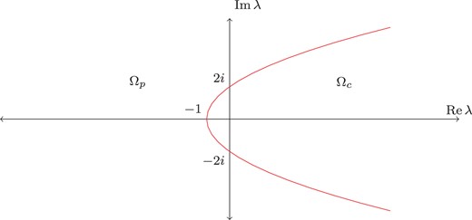
Fig. C.1.

A partition of the |$\lambda $|-plane for equation (1.3) with |$\nu =2$|⁠.

Open in new tabDownload slide

 

Remark C.1.

When |$\nu =2,$| we may represent graphically the |$L^2(0,1;r\,{d} r)$| nature of the solutions of (1.3); see Figure C.1. Here, |$\Omega _p:=\{\lambda \in \mathbb {C}\,|\,{\rm Im}\sqrt {\lambda }\geq 1\}$| and |$\Omega _c:=\{\lambda \in \mathbb {C}\,|\,{\rm Im}\sqrt {\lambda }<1\}$|⁠, so that if |$\lambda \in \Omega _p$| or |$\Omega _c,$| then equation (1.3) is, respectively, in PLP or PLC.

 

Lemma C.3.

Consider equation (1.3) with real-valued|$w,q\in L^1_{{\rm loc}}(0,1]$|. Let|$0\leq \nu <2$|. Define|$\varepsilon _1(r) = r^\nu w(r)-1$|and|$\varepsilon _2(r) = q(r)/w(r),$|and suppose that

\begin{equation} \varepsilon_j(r) =o(1)\quad (r\longrightarrow 0,\ j=1,2). \end{equation}

(C.7)

Then there is a fundamental system|$\{u_1(\cdot \,;\lambda ),u_2(\cdot \,;\lambda )\}$|satisfying|$u_1(r;\lambda )\rightarrow 1,u_2(r;\lambda )\sim \log (r)$|as|$r\rightarrow 0,$|and both|$u_1$|and|$u_2$|are in|$L^2(0,1;r\,{d} r)$|.

 

Proof.

Transform by |$v(r)=r^{1/2}u(r)$|⁠, so that (1.3) becomes

\begin{align} -v''(r;\lambda)-\frac{1}{4r^2}v(r;\lambda) &=(\lambda w-q)(r)v(r;\lambda) \notag\\ &=r^{-\nu}(1+\varepsilon_1(r))(\lambda-\varepsilon_2(r))v(r;\lambda). \end{align}

(C.8)

Consider the sequences |$(v_k(\cdot \,;\lambda ))_{k=0}^\infty $| and |$(y_k(\cdot \,;\lambda ))_{k=0}^\infty $| defined by

\[ -v_{k+1}''(r;\lambda)-\frac{1}{4r^2}v_{k+1}(r;\lambda) =(\lambda w-q)(r)v_k(r;\lambda), \]

and an equation of the same form for |$y_k$|⁠, satisfying |$v_0(r;\lambda )=r^{1/2}$| and |$y_0(r;\lambda )=r^{1/2}\log (r)$|⁠.

We now suppress the |$\lambda $|-dependence to simplify notation. If we can show that the series (note, starting from |$k=1$|⁠) |$V:=\sum _{k=1}^\infty v_k$| and |$Y:=\sum _{k=1}^\infty y_k$| converge uniformly near 0, and satisfy the asymptotics

\begin{equation} V(r)=o(r^{1/2}),\quad Y(r)=o(r^{1/2}\log(r))\quad (r\longrightarrow 0), \end{equation}

(C.9)

then |$r^{-1/2}v=r^{-1/2}v_0+r^{-1/2}V$| and |$r^{-1/2}y=r^{-1/2}y_0+r^{-1/2}Y$| is the required solution pair.

Note that |$v_0,y_0$| form a fundamental system in the kernel of the left-hand side of (C.8), and their Wronskian is 1. Therefore, by variation of parameters, |$v_k$| (and |$y_k$| in place of |$v_k$|⁠) must satisfy

\begin{align*} v_{k+1}(r) &=\int_0^r(v_0(r)y_0(s)-y_0(r)v_0(s))(\lambda w-q)(s)v_k(s) \,{d} s \notag\\ &=r^{1/2}\int_0^rs^{1/2-\nu}(\log(s)-\log(r)) (1+\varepsilon_1(s))(\lambda-\varepsilon_2(s))v_k(s)\,{d} s. \end{align*}

We want to estimate this integrand. By (C.7), this is straightforward. For each fixed |$\lambda $| there is |$\delta _1>0$| such that

\begin{equation} |(1+\varepsilon_1(r))(\lambda-\varepsilon_2(r))|<2|\lambda|\quad (0<r<\delta_1). \end{equation}

(C.10)

Furthermore, there is |$\delta _2>0$| with

\begin{equation} |{\rm log}(r)|<r^{-1+\nu/2}\quad (0<r<\delta_2). \end{equation}

(C.11)

Take |$\delta (\varepsilon )=\min \{\delta _1,\delta _2\},$| where |$\varepsilon =1-\nu /2>0$|⁠.

We first consider |$v_k$|⁠. By the triangle inequality, (C.10) and (C.11), we have the estimate

\[ |v_{k+1}(r)|\leq2|\lambda|r^{1/2}\left\{\int_0^rs^{\varepsilon-3/2}|v_k(s)|\,{d} s +r^{-\varepsilon}\int_0^rs^{2\varepsilon-3/2}|v_k(r)|\,{d} s\right\}\ (0<r<\delta,\ k=0,1,2,\ldots). \]

From this and |$|v_0(r)|\leq r^{1/2}$|⁠, we derive inductively that

\begin{equation} |v_k(r)|\leq\frac{(3/2)_k}{(k+1)!k!}r^{1/2} \left(\frac{4|\lambda|r^\varepsilon}{\varepsilon}\right)^k\quad (0<r<\delta,\ k=1,2,3,\ldots), \end{equation}

(C.12)

where |$(z)_k=z(z+1)\cdots (z+k-1)$| is the Pochhammer symbol. But, for all |$j\geq 0,$| we have

\[ \frac{3/2+j}{2+j}<1 \implies \frac{(3/2)_k}{(k+1)!}<1\quad (k\in\mathbb{N}). \]

Thus (C.12) simplifies to

\begin{equation} |v_k(r)|<r^{1/2}\frac{1}{k!}\left(\frac{4|\lambda|r^\varepsilon}{e}\right)^k\quad (0<r<\delta,k\in\mathbb{N}), \end{equation}

(C.13)

implying, by Weierstrass' M-test for convergence of functional series, that |$V$| is uniformly convergent on the interval |$(0,\delta )$|⁠. Furthermore, by (C.13), all terms in |$V$| are |$O(r^{1/2+\varepsilon })=o(r^{1/2})$|⁠, so one-half of (C.9) is satisfied; it follows that |$v(r)=r^{1/2}(1+O(r^\varepsilon ))~(r\rightarrow 0)$|⁠, as required.

We appeal to a similar argument in the case of |$y$|⁠, using (C.10) alongside the slightly different estimates

\begin{align*} |{\rm log}(r)| &<r^{-\varepsilon/2}\quad (0<r<\delta(\varepsilon/2)), \\ |y_1(r)| &\leq\frac{10|\lambda|r^{1/2+\varepsilon}}{3\varepsilon}\quad (0<r<\delta(\varepsilon/2)), \\ |y_{k+1}(r)|&\leq2|\lambda|r^{1/2}\left\{\int_0^rs^{\varepsilon-3/2}|y_k(s)|\,{d} s +r^{-\varepsilon}\int_0^rs^{2\varepsilon-3/2}|y_k(s)|\,{d} s\right\}\quad (0<r<\delta(\varepsilon),k\in\mathbb{N}). \end{align*}

These can be used inductively to show that

\[ |y_k(r)|\leq\frac{2(3/2)_k}{(k+1)!k!}r^{1/2} \left(\frac{4|\lambda|r^\varepsilon}{\varepsilon}\right)^k\quad (0<r<\delta(\varepsilon/2),k\in\mathbb{N}). \]

Thus, as with |$v_k$|⁠, the series |$Y$| is uniformly convergent on |$(0,\delta (\varepsilon /2))$|⁠, and the estimates show that the remaining half of (C.9) is satisfied: |$Y(r)=O(r^{1/2+\varepsilon })=o(r^{1/2}\log (r))$|⁠.

The last claim is that both |$u_1(r)=r^{-1/2}v(r)$| and |$u_2(r)=r^{-1/2}y(r)$| are in |$L^2(0,1;r\,{d} r)$|⁠. Clearly, for any |$\delta >0$|⁠, on the interval |$(\delta ,1)$| the equation (1.3) is regular, so its solutions are all continuous. We now see that |$u_1(r)\rightarrow 1,u_2(r)\sim \log (r)$| as |$r\rightarrow 0$|⁠, so the claim follows immediately. □

References

Author notes