Capital Assembly Free

Abstract

1. Introduction

This article explores the problem of assembling capital for projects. Under the usual economic assumption of decreasing-returns-to-investment, this problem does not arise; but when there are increasing returns over some range, investors may only be willing to invest in projects when they believe others are willing to do so. In such instances, assembling capital (or coordinating investors) is a relevant—and often critical—consideration. This article addresses the issue by viewing the process of assembling capital as part of the equilibrium, and it explores the consequences of capital assembly for a range of features of investment. One striking implication is that investors with blocks of capital will serve as anchor investors for projects and earn higher rates of return than small investors. Our theory also predicts that certain agents who possess a privileged network position can use their “network capital” to improve overall investment and they receive outsize returns for doing so. Our theory speaks to a fundamental aspect of the investment process that existing models fail to address. In contrast to existing theories, which assume surplus maximization, we emphasize the importance of scarce resources, such as block capital, for the execution of valuable projects. This implies that these resources earn rents—potentially large ones—in market equilibrium. It also implies that institutions may be important, as they may affect the supply of these scarce resources, and hence the extent to which valuable projects are implemented.

We analyze a model in which a project owner tries to raise capital for a project that exhibits increasing returns over some range. We first show that by making an anchor investment in the project, a large investor with a block of capital can move the project from a “bad” equilibrium with low investment to a “good” equilibrium with high investment. Since large investor spurs others to invest by making an anchor investment, he need not finance the entire shift to the good equilibrium himself. We characterize the minimum capital block-size needed to effect a shift to the good equilibrium—as well as the rate of return earned on such an investment. Interestingly, by holding a subordinated claim rather than a senior claim (equity or junior debt), a large investor can move the project to the good equilibrium with a smaller block of capital.¹ We also consider the possibility that a central network actor might substitute for block capital by coordinating small investors.

A key goal of the article is to develop a simple approach to the problem of capital assembly and increasing returns that can be applied in a variety of settings. The details of our analysis, while subtle, can largely be ignored once they have been considered. Our formal model is game-theoretic; but it boils down to a model that is essentially price-theoretic. We present this simpler, price-theoretic treatment in Section 2 and our formal model in Section 3.

There are many “real-world” examples that illustrate the capital-assembly problem. For instance, Warren Buffett’s investment in Goldman Sachs demonstrates the power of blocks of capital. In September 2008, soon after the collapse of Lehman Brothers, Buffett provided Goldman with $5 billion—an investment that greatly increased market confidence in the firm’s ability to weather the financial crisis. On the back of Buffett’s investment, Goldman raised an additional $2.5 billion from smaller investors. The deal was made on very favorable terms to Buffett. Berkshire Hathaway (Buffett’s company) received a 10% annual dividend on its “perpetual preferred” stock, plus warrants to buy $5 billion of common stock at 8% below the previous day’s closing price.² By comparison, the investors who provided the additional $2.5 billion did not receive nearly as favorable terms.

The founding of Federal Express, by Fred Smith, provides another example. A sizable amount of capital was required to start the company. Before FedEx could even open its doors, it needed to have in place a fleet of jets, a central hub with sorting facilities, pickup and delivery operations in a large number of cities (initially, 25), and several hundred trained employees. Moreover, FedEx operated at a loss for its first three years while demand for its service grew, in which time the company lost $40 million. Smith had some initial seed capital (his own trust fund being one source), which he quickly burned through, after which he faced a freeze from investors. The situation became dire, with creditors threatening to stop supplying materials and airports threatening to impound planes.³ In a last-ditch effort, Smith met with the wealthy industrialist Henry Crown, founder of General Dynamics. Crown agreed to guarantee a $23.7 million loan from Chase. This block investment helped Smith raise an additional $52 million and got the company through the critical period where it was operating at a loss. Crown’s terms, like Buffett’s, were tough. They included, for instance, an option to acquire control of Federal Express (an option which, fortunately for Smith, was never exercised).

There is empirical support for the idea that network connections yield substantial returns. Hochberg et al. (2007), for instance, find that socially connected venture capital (VC) firms do especially well. The VC industry, in general, is characterized by strong network ties among VC firms that typically syndicate their deals with others. Hochberg et al. (2007) find that the “centrality”⁴ of VCs in their network increase their internal rates of return from 15% to 17% for a one-standard deviation increase in centrality. Similarly, they find that the more central a VC firm, the better the performance of its portfolio companies. A one standard deviation change in VC centrality increases the probability that a portfolio company survives its first funding-round from 66.8% to 72.4%. A possible interpretation of their findings is that VC firms provide startups with network capital in exchange for a share of their returns. Indeed, the well-known venture capitalist Marc Andreessen sees his main role as to “give our founders … networking superpower.”⁵

Outside of economics, sociologist Ronald Burt pioneered the idea that social capital matters for finance and entrepreneurship (see Burt 2004). More recently, economists have begun to explore the role of social capital for finance (see Guiso et al., 2004; Hong et al., 2004, 2005; and Gompers et al., 2005). We see our article as contributing to this (still nascent) literature.

The most closely related paper is Akerlof and Holden (2016). In that paper, we consider a specific setting in which a networked agent—a “mover and shaker”—can increase aggregate investment and earn a rent. This article gives a more general treatment of the capital-assembly problem; it is also much simpler. We accomplish this by stripping out informational considerations and focusing squarely on agents’ coordination problem (using a risk-dominance-style refinement rather than a global-games approach). Our methodology does not require us to make assumptions about the shape of production functions. It reveals the importance of block capital as well as network capital for coordinating investors. Importantly, we are also able to embed our analysis within a market and study the nature of equilibrium: both how block capital and network capital are deployed and the rents they command.

Our article also relates to Murphy et al. (1989), who explore the idea that increasing returns can generate multiple equilibria. They propose this as a reason for poverty traps.⁶

There is a large literature in corporate finance on the value of controlling blocks and large shareholders (see Grossman and Hart 1980 and Shleifer and Vishny 1986 for early contributions and Becht et al. 2003 for further discussion and references). In these models, the value of large stakes comes from control rights; but there is scant consideration of the coordination problems involved in raising capital.

Our article connects to the literature on contribution games—especially Andreoni (1998). In a charitable-giving context, he considers the role of a large contributor or government in achieving successful coordination.⁷ Relative to Andreoni (1998), the novel features of our analysis are our focus on an investment context and our examination of the rents associated with playing a pivotal role in coordination.⁸

Building on the work of Segal (1999), who initiated a literature on contracting with externalities, Bernstein and Winter (2012) and Sakovics and Steiner (2012) study settings where large players can earn rents because of the positive externalities they impose on smaller players. An example would be a shopping mall operator offering a discounted rental rate to a national brand store due to its importance in driving traffic to smaller stores.⁹

Finally, in subsequent work, Halac et al. (2018) study a model similar to ours. Their contribution relative to our work is to investigate, in the spirit of Andreoni (1998), mechanisms that guarantee a unique Nash equilibrium.¹⁰ Focusing on such mechanisms is relevant, for instance, when the principal is infinitely risk-averse and so, when facing multiple equilibria, fears a terrible outcome; or when (as in our model) the least preferred equilibrium is especially likely to arise.¹¹

The remainder of the article is organized as follows. Section 2 gives the simple price-theoretic treatment of our model. Section 3 develops the model more formally. We first examine the role a large investor can play in assembling capital for a project; we then embed our analysis in a market setting (with multiple projects) and analyze the market equilibrium; finally, we discuss how network capital might substitute for block capital. Section 4 considers some issues raised by our theory and Section 5 concludes. Formal proofs are contained in the Appendix.

2. A Simple Treatment of the Capital-Assembly Problem

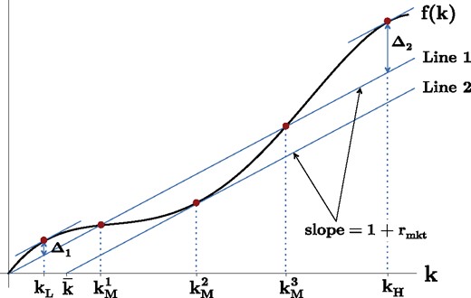
Imagine a project owner is trying to assemble capital for a project. When k units of capital are invested in the project, it yields a return f(k). Our theory can handle production functions with any shape; for the purposes of illustration, though, assume f(k) has the shape shown in Figure 1.¹² The production function in Figure 1 exhibits increasing returns for intermediate values of k and decreasing returns for high and low values of k.

Figure 1.

An Example.

Open in new tabDownload slide

Case 1: Small Investors Only

Suppose there are many risk averse investors, each with only a small amount of capital. They can invest in the project or earn a market rate of interest, r_mkt.

We will show in the next section that there are two equilibria, one good and one bad; however, the bad equilibrium is likely to prevail. In the bad equilibrium, the project owner obtains k_L units of capital at the market interest rate and receives a payoff of $Δ1$⁠. In the good equilibrium, the project owner receives the surplus-maximizing amount of capital, k_H, at the market interest rate and receives a payoff of $Δ2>Δ1$⁠.

Why is the bad equilibrium likely to prevail? Observe that there is a region in which the project is in the “red,” yielding an insufficient return to pay off investors (⁠$f(k)<(1+rmkt)k$⁠). In Figure 1, this is the region between $kM1$ and $kM3$⁠, in which f(k) dips below Line 1. Investors take a risk when they try to coordinate on lending k_H rather than k_L, since the project may end up in the region in which it is undercapitalized and in the “red.” In game-theoretic terms, the bad equilibrium “risk dominates” the good one. There is a large literature showing that risk dominant equilibria tend to be focal.¹³

To summarize, we find that a bad equilibrium, with a k_L-level of investment, is likely to prevail when capital is disaggregated (i.e., investors have only negligible amounts of it).

Case 2: One Large Investor

Let us assume now that, in addition to small investors, there is a large investor with a block of capital of size k_block.

A large investor with a block of capital can potentially ensure the optimal level of investment (k_H). It is obvious that he can do so if $kblock≥kH$⁠; but he may be able to bring about the optimal level of investment even if he is unable to fund the entire project. For instance, a block of size $kM3−kM1$ is adequate. Small investors are happy to lend when the project is in the “black”; there is only reluctance to lend between $kM1$ and $kM3$⁠, when the project is in the “red.” A block of size $kM3−kM1$ is enough to bridge this gap.

In fact, it turns out that the large investor can bring about the good equilibrium with less capital still. It is sufficient to have a block of size $k¯$ (⁠$k¯$ is graphically represented in Figure 1). Suppose the large investor loans $k¯$ for the project and, additionally, enables the project owner to pay off small investors first. (This could be achieved either by taking junior debt or equity in the project.) Small investors are paid off in this scenario so long as f(k) does not dip below Line 2. f(k) is tangent to Line 2 at $kM2$ but never dips below; hence, small investors are certain to be paid off. Since small investors need not worry about being paid off, they will be willing to provide the project owner with the additional capital he needs to reach the good equilibrium.

Therefore, a large investor with a block of size $kblock≥k¯$ can generate a surplus of size $Δ2−Δ1$⁠.

Market Rates of Return: Large Versus Small Investors

Consider next a market setting, with many projects, in which interest rates are endogenous. In a competitive capital market, if block capital is scarce, large investors earn higher rates of return than small investors. Large investors receive, in addition to r_mkt, the surplus their blocks help generate.

When projects are scarce as well as block capital, the rent distribution may be different. Project owners may capture some rents as well as block holders. Block capital is nonetheless critical for achieving efficient outcomes.

Network Capital

Suppose investors are networked. It might be possible for a central network actor (C) to use his position to coordinate small investors on a high level of investment. Agent C substitutes for a block investor; hence, he should earn an equivalent rent in a market equilibrium (i.e., $Δ2−Δ1$ if the block investor for which he substitutes receives a rent of $Δ2−Δ1$⁠).

We can think of agent C as possessing “network capital” and we can think of $Δ2−Δ1$ as the rent agent C earns on his network capital.

3. The Formal Model

This section develops the model more formally. It is organized along similar lines to Section 2. Sections 3.1 through 3.4 consider a setting in which a project owner is trying to raise capital from investors. We initially assume that there are only small investors; we then show that a large investor can improve the overall level of investment. Section 3.5 moves to a market setting, with many projects, and examines the market equilibrium. Interest rates are endogenous (in contrast to Sections 3.1 through 3.4).

3.1 Setup

The owner of a project is trying to raise capital from a set of potential investors (⁠$i∈{1,2,…,n}$⁠). Each investor possesses a small amount of capital, δ.

At time 1, the project owner decides (i) how much capital he will try to raise (⁠$kP≥0$⁠) and (ii) the interest rate (⁠$rP≥0$⁠) he will pay to those who invest in the project. We assume the project owner’s capital target, k_P, must be a multiple of δ (⁠$kP∈{0,δ,2δ,3δ,…}$⁠).

At time 2, after observing the project owner’s choices, potential investors simultaneously decide under what circumstances they are willing to invest in the project. Each investor chooses $ai(κ)∈{0,1}$ for all values of $κ<kP$ that are multiples of δ. $ai(κ)=1$ indicates that investor i is willing to invest if the project owner has raised κ units of capital at the point he approaches i.

At time 3, the project owner approaches investors in a random order. Agent i becomes an investor in the project if, when approached, he is willing to invest (⁠$ai(κ)=1$⁠) and the project owner has yet to meet his capital target k_P (⁠$κ<kP$⁠). Let k denote the total amount of capital raised at time 3.¹⁵

At time 4, the project yields a return f(k). The project owner receives $f(k)−(1+rP)k$ when the project is in the “black” (i.e., when $f(k)−(1+rP)k≥0$⁠) and 0 when the project is in the “red.” Agents who invested in the project receive a rate of return r_P when the project is in the “black”; they receive equal shares of f(k) when the project is in the “red,” with an associated rate of return $f(k)k−1$⁠. Agents who do not invest in the project receive the market rate of interest, r_mkt.

The project owner is risk neutral. Investor i’s utility is given by $u(wi)$⁠, where w_i denotes the final wealth of investor i. u is strictly increasing and weakly concave: $u′>0,u″≤0$⁠. w_i is equal to $δ(1+ri)$⁠, where r_i is investor i’s rate of return. As a tie-breaking rule, we assume, for ease of later exposition, that investors prefer all else equal to choose $a(κ)=1$ when there is a positive probability of being approached by a project owner who has raised κ and $a(κ)=0$ otherwise.¹⁶

We make a set of simplifying assumptions regarding f(k). Under these assumptions, f(k) resembles the production function in Figure 1. Later, we will discuss how our analysis can be generalized. Let $π(k)=f(k)−(1+rmkt)k$⁠. We assume:

1. $π(k)$ is continuous and $π(0)=0$⁠.

2. $π(k)$ has its global maximum at $kH≤nδ$ and $π(kH)=Δ2$⁠.

3. $π(k)$ also has a local maximum at k_L < k_H and $π(kL)=Δ1$⁠.

4. $π(k)<0$ if and only if $kM1<k<kM3$⁠, where $kL<kM1<kM3<kH$⁠.

5. $π(k)$ has its global minimum at $kM2$ and $π(kM2)=−Δ3$⁠.

6. $δ<min(kL,Δ31+rmkt,kM3−kM1−Δ31+rmkt)$⁠.

7. k_L, k_H, $kM1, kM2, kM3$⁠, and $Δ31+rmkt$ are all multiples of δ.¹⁷

3.2 Analysis

Let us compare two strategies the project owner might follow. Strategy 1: set out to raise k_L at the market rate of interest (k_P = k_L and $rP=rmkt$⁠). Strategy 2: set out to raise k_H at the market rate of interest (k_P = k_H and $rP=rmkt$⁠). (We will later discuss whether there might be a third strategy that is preferable to these two.)

First, consider what happens when the project owner follows Strategy 1. 

The project owner only seeks to raise k_L and the project is in the black for all $k≤kL$⁠. Therefore, the project owner has no trouble raising k_L from investors.

Now, consider what happens when the project owner follows Strategy 2. 

The time-2 subgame is a coordination game with two equilibria. In Equilibrium 1, investors are willing to invest up to the point the project dips into the red (⁠$ai(κ)=1$ if and only if $κ<kM1$⁠); this results in the project owner raising $kM1$⁠. In Equilibrium 2, investors are willing to invest even when the project is in the red (⁠$ai(κ)=1$ for all κ); this results in the project owner raising k_H.

Observe that Strategy 1 yields a higher payoff if Equilibrium 1 prevails, whereas Strategy 2 yields a higher payoff if Equilibrium 2 prevails. As we will see presently, Equilibrium 1 involves less strategic risk than Equilibrium 2. Therefore, the project owner has good reason to think Equilibrium 1 will prevail and he has good reason to select Strategy 1.

Harsanyi and Selten (1988)’s concept of risk dominance captures the idea that certain equilibria in coordination games may involve less strategic risk than others. Suppose a (symmetric) 2 × 2 coordination game has two pure-strategy Nash equilibria, (U, U) and (D, D). Players may be uncertain whether the other player intends to play U or D. Harsanyi and Selten say that (U, U) risk dominates (D, D) if players prefer to play U when the other player chooses U with probability $12$ and D with probability $12$⁠.

Harsanyi and Selten’s original article focuses on a limited class of games; however, an equilibrium concept proposed by Kets and Sandroni (2017)—“introspective equilibrium”—is more general.¹⁸ Introspective equilibrium is based upon level-k thinking (see Crawford et al. 2013 for a survey). Kets and Sandroni assume that each player has an exogenously-given “impulse” which determines how he plays at level 0. At level k > 0, each player formulates a best response to the belief that opponents are at level k – 1. Introspective equilibrium is defined as the limit of this process as $k→∞$⁠. A formal definition follows. 

Under these assumptions, Equilibrium 1 is the unique introspective equilibrium of the time-2 game (see Proposition 3). In this sense, it risk dominates Equilibrium 2. 

Hence, when investors follow the introspective equilibrium, the project owner prefers Strategy 1 to Strategy 2. A remaining question is whether there might be a Strategy 3 that the project owner prefers to both Strategies 1 and 2. Clearly, it would not be optimal to offer an interest rate below the market rate since this leads to zero investment. It might be optimal, though, to offer a rate greater than r_mkt. Doing so might get agents to overcome their fear of investing in the project when it is in the red. Specifically, Strategy 3 would involve offering an interest rate $r˜>rmkt$ and seeking to raise $k˜=arg maxk[f(k)−(1+r˜)k]$⁠.

Proposition 4 (stated below) says that, if agents are sufficiently risk averse, Strategy 1 is optimal.²⁰ There are two reasons for this result. First, if agents are sufficiently risk averse, no above-market interest rate will induce agents to invest when the project is in the red. Second, even if it is possible to induce agents to invest in the project when it is in the red, it may require paying a high interest rate. If $r˜$ is large, the project owner’s payoff from raising $k˜$ at rate $r˜$ will be less than the payoff from following Strategy 1 (⁠$Δ1$⁠). In other words, the cost to the project owner of paying the higher interest rate may exceed the benefit. 

Henceforth, we will assume that investors follow the introspective equilibrium. We will also focus on the case where Strategy 1 is optimal. We focus on this case for simplicity; but a version of our argument regarding the value of block capital goes through even when Strategy 3 is optimal. In that case, block capital reduces the interest rate the project owner needs to pay to small investors.

3.3 A Large Investor

Suppose that, in addition to small investors, there is one large investor with a block of capital of size k_block (where k_block is a multiple of δ). The large investor has the same utility function as small investors; and, like small investors, his outside option yields a rate of return r_mkt. At time 1, the large investor can make a loan to the project owner. A loan contract between the project owner and the large investor specifies five things:

1. The loan size (⁠$klarge≤kblock$⁠).

2. The interest rate (r_large).

3. Whether the loan is junior seniority or standard seniority.

4. The point at which the loan is to be made (κ_large).

5. The amount of capital the project owner will try to raise from small investors (k_P) and the interest rate he will pay them (r_P).

Points 3 and 4 require further elaboration. We assume the loan can either be junior seniority or standard seniority. If it is junior seniority, the large investor gets paid off after small investors. If the loan is standard seniority, the large and small investors have the same seniority; when the project is in the red, the large investor receives a fraction of f(k) proportional to the amount of capital he loaned (⁠$klargek$⁠).

κ_large denotes the point at which the large investor makes a loan. We assume that the large investor puts k_large into the project at the point the project owner has raised κ_large from small investors. If the project owner never manages to raise κ_large from small investors, the large investor does not put capital into the project and he earns the market rate of interest on k_block.

We assume that the project owner and the large investor engage in Nash bargaining over the contract and have equal bargaining power.

Analysis

If a large investor has sufficient capital, he can help the project owner reach k_H. For instance, if $kblock≥kH$⁠, the large investor can loan the project owner all the capital he needs (⁠$klarge=kH$⁠).

It is natural to ask how large k_block must be in order for the large investor to help the project owner reach k_H. First, suppose the large investor makes a standard-seniority loan. A block of size $kM3−kM1−δ$ is sufficient in this case. The large investor can lend $kM3−kM1−δ$ after the project owner has raised $kM1$ from small investors (⁠$klarge=kM3−kM1−δ$ and $κlarge=kM1+δ$⁠), thereby bridging the region where the project is in the red and small investors are unwilling to invest. If the block size is any smaller, though, it is impossible to reach k_H.

Now suppose the large investor makes a junior-seniority loan. To reach k_H, the block only needs to be large enough to ensure that small investors are paid off. It is easily shown that the minimum block-size that is sufficient to reach k_H is $k¯=Δ31+rmkt$ and $k¯<kM3−kM1−δ$⁠. The block can be invested before—or just after—the project owner has raised $kM1$ from small investors: $κlarge≤kM1+δ$⁠.

This leads to Proposition 5. 

Discussion

We have assumed that the large investor makes his investment decision before small investors (at time 1 rather than time 2). This raises the question whether the rents earned by the large investor are a consequence of his size or the order in which he is approached.

Observe that the large investor is the only investor who values being approached first. A small investor would not value moving first since he cannot, through an anchor investment, help the project owner reach k_H. In contrast to small investors, if the large investor moves early, he reduces strategic uncertainty for other investors and thereby increases their willingness to invest. Furthermore, by reducing the strategic uncertainty faced by small investors, the large investor reduces the strategic uncertainty he himself faces.

Therefore, even if the large investor must compete for the right to invest first, one would expect him to win this right—and at low cost. For instance, if the right to move first is determined through a second-price auction, the large investor will win the auction and pay zero since he is the only investor who positively values the right.²²

3.4 Other Production Functions

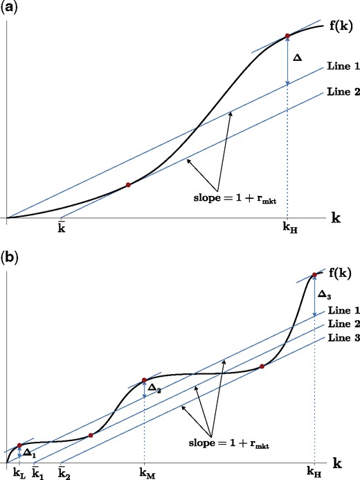
For ease of exposition, we restricted attention to production functions resembling the one in Figure 1. Our analysis easily extends to other production functions.

For instance, Figure 2a shows a production function that exhibits increasing returns for low values of k rather than intermediate values of k. There is still a “good” equilibrium and a “bad” equilibrium. In the bad equilibrium, zero capital is invested in the project. In the good equilibrium, k_H is invested in the project. The good equilibrium generates a surplus of Δ; a block of capital of size $k¯$ is needed in order to reach it since f(k) dips into the red—down to Line 2—between k = 0 and k = k_H.

Figure 2.

Other Types of Production Functions.

Open in new tabDownload slide

Figure 2b shows a more complicated production function. $π(k)=f(k)−(1+rmkt)k$ has three local maxima—at k_L, k_M, and k_H. The project owner can reach k_L without any help from a block investor because the project is in the black for all $k≤kL$⁠. To reach k_M, the project owner must obtain some help from a large investor since the project dips into the red between k_L and k_M. The project dips down to Line 2 and hence a block of size $k¯1$ is required to reach k_M. To reach k_H, the project owner must obtain a larger block (of size $k¯2$⁠) because the project dips further into the red—down to Line 3—between k_M and k_H.

Proposition 6 provides a more formal statement of how our results generalize. 

3.5 Market Equilibrium

Our focus thus far has been on a single project and we have taken interest rates as exogenous. It is natural at this point to consider a market setting with many projects, in which interest rates are endogenous, and ask what a market equilibrium might look like.

A benchmark case to consider is a market with the following features:

1. There are multiple types of projects (where a project’s type is defined by its production function); there are many projects of any given type.

2. Each project has a different owner.

3. A set of potential investors possess blocks of capital of varying sizes.

4. Potential investors prefer to invest their capital—rather than consume it—if they can earn an interest rate greater than or equal to r₀.

5. In aggregate, potential investors possess an infinite (or very large) amount of capital.

6. Block capital is scarce, however: for any k, there is a finite amount of capital in blocks of size k or greater.

What can we say about the market equilibrium? First, an investor’s rate of return will depend upon the size of his capital block. Let $rmkt(k)$ denote the rate of return on a block of size k.

Third, there will be some threshold, $k^$⁠, such that $rmkt(k)=r0$ for $k<k^$ and $rmkt(k)>r0$ for $k≥k^$⁠. Investors with blocks of size $k^$ or greater will serve as anchor investors for projects and thereby earn more than r₀. Investors with smaller blocks will not serve as anchor investors.

Finally, blocks will be deployed in equilibrium on the projects that maximize the size of the associated surplus (⁠$Δ2−Δ1$⁠). Given the scarcity of block capital, many projects will be undercapitalized in equilibrium. Furthermore, depending upon block interest rates, a project of the type shown in Figure 2b might be funded up to k_M (rather than k_L or k_H).²³

Assumptions 1–6 are clearly strong and it is important to remember that they are only meant to serve as a benchmark. In particular, one could imagine settings where there are relatively few projects or where block capital is abundant. In such a setting, $Δ2−Δ1$ might by partially or wholly captured by the project owner.²⁴

Network Capital

If investors are networked, a central network actor might be able to substitute for block capital. The central actor might be able to use his position to coordinate small investors on a high level of investment (for instance, by flipping their “impulses”). We would expect such central actors to earn rents on their “network capital” equivalent to those earned by large investors.²⁵

4. Discussion of the Model

In our model, block and network capital earn rents since they are scarce resources that are essential for capital assembly. A natural question is whether this finding is sensitive to the particular choice of modeling environment. We now consider a number of issues, in turn, that are potentially consequential.

First: could project owners and investors write conditional contribution contracts, whereby investors’ capital only goes into a project if the total amount pledged is above a threshold? Such contracts would seem to solve the capital-assembly problem; hence one might expect to see them with great regularity. We do, in fact, see such contracts: “Kickstarter” being a notable example. However, conditional contribution contracts are far from ubiquitous, and this begs the question as to why. One reason is that it is usually easy to walk away from such pledges. An escrow account might help but such accounts are known to be far from airtight. Furthermore, there is an incentive to wait to contribute to see what other investors will do, which leads to a problem of a “race to the last.” Waiting retains one’s option value; and there is also an informational benefit of waiting.

Second: there would seem to be an incentive for project owners to start projects only after they have finished raising capital. A project owner who tries but fails to raise k_H could thereby invest only k_L in the project and return the remaining capital to investors. Although delaying the start of a project can help solve the capital-assembly problem, there may be large costs associated with delay. Furthermore, project delay may send a negative signal to investors regarding a project owner’s ability to raise capital.²⁶

Third: arguably, the project owner faces strategic risk (not just investors). Put differently, in our model, the project owner moves before investors and so is not part of the introspective equilibrium at time 2. For instance, suppose the project owner decides the capital target, k_P, at time 2 rather than time 1. In this case, continuing to approach investors past k_L (i.e., choosing k_P > k_L) is strategically risky for the project owner since he might fail to raise k_H and end up with a payoff below $Δ1$⁠. The large investor is even more vital in this setting since he allays the fears not only of investors but also of the project owner.²⁷

Fourth: one wonders whether the large investor solves the coordination problem merely by his presence. Even without investing, small investors’ fears might be allayed by the thought that the large investor will do so should the project run into trouble. The large investor must actually make an anchor investment to solve the coordination problem if small investors believe there is even a small chance the large investor will disappear. In a market setting, furthermore, large investors are unlikely to stay around in perpetuity as there are alternative projects in which they can invest.

Fifth: our model suggests that small investors might want to contract with a proxy to act on their collective behalf. The proxy would allow the small investors to behave as if they were a single, large investor. Arguably, private equity and activist hedge funds play such a role. An issue, however, is that it may be hard to align the proxy’s interests with those of small investors. Such moral hazard considerations explain, for instance, why there are typically limits placed on the size of single investments, and the class of securities in which fund managers can invest.

Sixth: our model assumes that small investors commit to an investment policy. In the absence of commitment, the “bad” equilibrium can unravel. If the project owner tries to raise k_H, the last investor needed to reach k_H will invest; the second-to-last investor, recognizing this, will invest; by iteration, all investors are prepared to invest. This unraveling argument is fragile, however. For instance, it falls apart if the project’s return (f(k)) is not strict common knowledge.²⁸

Seventh: We have assumed that small investors do not condition their strategies on the order in which they are approached. This may be a realistic assumption since investors may not know who has been approached before them. However, were investors able to condition their strategies on order (i.e., $ai(κ,order)$⁠), it would not change conclusions. In this case, there is an analog of Proposition 3 in which the project owner only raises $kM1$ from small investors when he sets out to raise k_H.

Eighth: large investors in our model subordinate their claims to those of small investors (either by taking equity or junior debt in the project). This prediction is stark and may not perfectly reflect what we see in reality. The starkness of this prediction is an artifact, though, of our assumption that the project is riskless (i.e., our assumption that f(k) is non-random). Recall that a large investor subordinates his claim in our model because it reduces the amount of capital he needs to invest to bring about the “good equilibrium.” If the project is risky, however, there is an additional consideration. The large investor exposes himself to greater risk if he subordinates his claim. This second consideration might outweigh the first.

5. Concluding Remarks

In this article, we have examined the capital-assembly problem, which arises when there are increasing returns to investment. We have argued that holders of block capital play an important role in capital assembly. By serving as anchor investors for projects, they can increase the overall level of investment. Similarly, central network actors are important because they can use their position to coordinate small investors.

The potentially large returns earned by holders of block and network capital have implications for income inequality. Our theory also has implications for corporate finance. The problem we study may have a range of further implications. It is common (e.g., in growth theory) to assume that projects/ideas are in short supply. In contrast, the scarce resources in our theory are network and block capital. Our theory therefore shifts the focus from the challenge of generating ideas to the challenge of implementing and executing them.

Acknowledgement

We are grateful to the editor, Nicola Persico, and three anonymous referees for their detailed and thoughtful suggestions. We also thank George Akerlof, Pol Antras, Rosalind Dixon, Drew Fudenberg, Bob Gibbons, Ben Golub, Sanjeev Goyal, Hongyi Li, Luis Rayo, Jeremy Stein, and Luigi Zingales for helpful discussions, and seminar participants at Brown, Cambridge, LBS, Harvard, MIT, UC Irvine, UWA, Warwick, the Japan-Hong Kong-Taiwan Contract Theory Workshop, and the 10th Australasian Organizational Economics Workshop. R.A. acknowledges support from the Institute for New Economic Thinking (INET). R.H. acknowledges support from the Australian Research Council (ARC) Future Fellowship FT130101159.

Appendix

It is clearly an equilibrium for all investors to choose $a(κ)=1$ for all $κ<kP$⁠. Hence, an equilibrium exists in which the project owner raises k_L. Furthermore, this is the unique equilibrium in which the project owner raises k_L since, if the project owner is going to raise k_L, it is optimal for an investor to choose $a(κ)=1$ for all $κ<kP$ (given the tie-breaking rule).

We can prove by contradiction that an equilibrium does not exist in which the project owner raises less than k_L. Suppose the project owner raises $k^<kL$ in equilibrium with positive probability. Given that the project is in the “black” for all $k∈[0,kL]$ and given investors’ tie-breaking rule, investors will all choose $a(k^)=1$⁠. Therefore, if the project owner manages to raise $k^$⁠, investors always give him additional capital. It follows that the project owner can never raise exactly $k^$ (which is a contradiction). This completes the proof. □

We can prove by contradiction that an equilibrium does not exist in which the project owner raises $k^∈(kM1,kM3)$ with positive probability. Suppose such an equilibrium exists. Given that the project is in the “red” at $k^$⁠, investors’ payoffs are lower than they would be if they never invested in the project. Hence, investors are not best-responding (which is a contradiction).

We can also prove by contradiction that an equilibrium does not exist in which the project owner raises less than $kM1$⁠. Suppose the project owner raises $k^<kM1$ in equilibrium with positive probability. Given that the project is in the “black” for all $k∈[0,kM1]$ and given investors’ tie-breaking rule, investors will all choose $a(k^)=1$⁠. Therefore, if the project owner manages to raise $k^$⁠, investors always give him additional capital. It follows that the project owner can never raise exactly $k^$ (which is a contradiction).

Furthermore, by an analogous argument, an equilibrium does not exist in which the project owner raises $k^∈[kM3,kH)$ with positive probability.

To summarize, for all values of $k^$ except $kM1$ and k^H, we have ruled out that the project owner can raise $k^$ with positive probability in equilibrium.

Now, suppose the project owner raises $kM1$ with positive probability. Given that the project dips into the red when $k∈(kM1,kM3)$⁠, investors all prefer to choose $a(kM1)=0$⁠. If investors all choose $a(kM1)=0$⁠, the project owner cannot raise more than $kM1$⁠. Furthermore, we have already shown that an equilibrium does not exist in which the project owner raises less than $kM1$ with positive probability. Hence, if the project owner raises $kM1$ with positive probability in equilibrium, he raises $kM1$ with probability 1 in equilibrium.

At this point, we have shown that at most two types of equilibria exist: (1) an equilibrium in which the project owner raises $kM1$ with probability 1, and (2) an equilibrium in which the project owner raises k_H with probability 1. Let us now show existence of such equilibria.

It is clearly an equilibrium for all investors to choose $a(κ)=1$ for $κ<kM1$ and $a(κ)=0$ for $κ≥kM1$⁠. This results in the project owner raising $kM1$⁠. Furthermore, this is the unique equilibrium in which the project owner raises $kM1$ since, if the project owner is going to raise $kM1$⁠, it is optimal for investors to choose $a(κ)=1$ for $κ<kM1$ and $a(κ)=0$ for $κ≥kM1$ (given their tie-breaking rule).

It is also clearly an equilibrium for investors to choose $a(κ)=1$ for all κ. This results in the project owner raising k_H. Furthermore, this is the unique equilibrium in which the project owner raises k_H since, if the project owner is going to raise k_H, it is optimal for investors to choose $a(κ)=1$ for all κ (given their tie-breaking rule). This completes the proof. □

When investors are at level 0, they simply follow their impulses.

When investors are at level 1, they choose not to invest (⁠$ai(κ)=0$⁠) for $κ<kM3−δ$ and they choose to invest (⁠$ai(κ)=1$⁠) for $κ≥kM3−δ$⁠. The reason is as follows. When $κ≥kM3−δ$⁠, it makes sense to invest since there is no risk the project will end up in the “red.” (Furthermore, investors believe there is a positive probability they will be approached by a project owner who has raised $κ≥kM3−δ$⁠.) On the other hand, if investor i invests when $κ<kM3−δ$⁠, he believes there is a positive probability he will have invested in a project that ends up in the “red.” Consequently, it does not make sense to invest when $κ<kM3−δ$⁠.

When investors are at level 2, they choose to invest if and only if κ = 0. The reason is as follows. Since each investor believes other investors are at level 1, they believe there is zero probability of being approached by a project owner who has raised $κ>0$⁠. Investors choose $ai(κ)=0$ for $κ>0$ given their tie-breaking rule. On the other hand, there is a positive probability of being approached by a project owner who has raised κ = 0. Furthermore, there is zero probability of the project ending up in the “red” if investor i invests when κ = 0; hence, investor i will choose to do so.

When investors are at level 3, they choose to invest if and only if $κ≤δ$⁠. The reasoning is analogous to the reasoning for level 2. Given other investors are believed to be at level 2, investors assign zero probability to being approached by a project owner who has raised $κ>δ$⁠. Hence, investors choose $ai(κ)=0$ for $κ>δ$⁠. On the other hand, there is a positive probability of being approached by a project owner who has raised $κ≤δ$⁠. Furthermore, there is zero probability of the project ending up in the “red” if investor i invests when $κ≤δ$⁠; hence, investor i will choose to do so.

Applying the same logic, at level 4, investors will invest if and only if $κ≤2δ$⁠. At level 5, investors will invest if and only if $κ≤3δ$⁠. Eventually, we will reach a level $k^$ where investors invest if and only if $κ<kM1$⁠.

Observe that, at level $k^+1$⁠, investors follow that same strategy as at level $k^$⁠: they invest if and only if $κ<kM1$⁠. We conclude, then, that in the limit as $k→∞$⁠, investors’ strategy is to invest if and only if $κ<kM1$⁠. This results in the project owner raising $kM1$ units of capital in the introspective equilibrium. This completes the proof. □

When investors are at level 0, they simply follow their impulses.

Provided investors are sufficiently risk averse, at level 1 they choose not to invest for $κ<kM3−δ$ and they choose to invest for $κ≥kM3−δ$⁠. The reason is as follows. When $κ≥kM3−δ$⁠, it makes sense to invest since there is no risk of the project yielding investors a return below r_mkt (note: there is a risk still of the project yielding a return below $r˜$⁠). (Furthermore, investors believe there is a positive probability they will be approached by a project owner who has raised $κ≥kM3−δ$⁠). When $κ<kM3−δ$⁠, investors believe there is a positive probability that the project will yield them a return below r_mkt. There is also an upside risk to investing: the project yields investors a return above r_mkt with positive probability. However, if investors are sufficiently risk averse (i.e., $ρ>ρ¯$⁠), it follows from Jensen’s inequality that the downside risk will outweigh the upside risk and they will choose not to invest when $κ<kM3−δ$⁠.

The remainder of the proof follows along identical lines to the proof of Proposition 3. At level 2, investors choose to invest if and only if κ = 0 (see the proof of Proposition 3 for the reasoning). At level 3, investors choose to invest if and only if $κ>δ$⁠. Eventually, we reach a level $k^$ where investors invest if and only if $κ<kM1$⁠. For levels greater than $k^$⁠, investors follow the same strategy as at level $k^$⁠. Hence, we conclude that in the limit as $k→∞$⁠, investors’ strategy is to invest if and only if $κ<kM1$⁠. This results in the project owner raising $kM1$ units of capital in the introspective equilibrium.

Observe that the project owner’s payoff in equilibrium is 0. Hence, the project owner prefers Strategy 1 (which yields a payoff of $Δ1$⁠) to Strategy 3. This completes the proof. □

First, suppose $f(k)−(1+rmkt)(k−k¯)≥0$ for all values of $k≤k*$ that are multiples of δ. The large investor’s junior-seniority investment of size $k¯$ ensures that small investors cannot earn less than r_mkt if they invest in the project. Therefore, it is quite clear that, in the introspective equilibrium, small investors always invest (⁠$ai(κ)=1$ for all value of κ) and the project owner succeeds in raising $k*−k¯$⁠.

Now suppose $f(k)−(1+rmkt)(k−k¯)<0$ for some values of $k≤k*$ that are multiples of δ. Let $k^$ denote the minimum such value of k. Following an argument identical to that given in the proof of Proposition 3, the introspective equilibrium involves agents agreeing to invest if and only if $κ<k^−δ$⁠. Hence, the project owner only raises $k^−δ$ units of capital from small investors. This completes the proof. □

Footnotes

References