


Abstract
We utilize data from sensitive soccer games in 75 countries between the years 2001 and 2013. In these games one team was in immediate danger of relegation to a lower division (Team A) and another team was not affected by the result (Team B). Using within-country variation, our difference-in-difference analysis reveals that the more corrupt the country, according to Corruption Perceptions Index, the higher is the probability that Team A would achieve the desired result in the sensitive games relative to achieving this result in other, non-sensitive games against the same team. We also find that in the later stages of the following year, the probability that Team A would lose against Team B compared to losing against a similar team (usually better than Team B) is significantly higher in more corrupt countries than in less corrupt countries. This result serves as evidence of quid pro quo behavior. (JEL A12, D73, C93, Z20)
1. Introduction
In recent years there is a growing interest among economists to study the relationship between social norms and corrupt behavior. In a pioneering cross-country field experiment, Fisman and Miguel (2007) found that United Nations diplomats living in New York who represent governments from very corrupt countries accumulated significantly more unpaid parking violations than their counterparts from less corrupt countries. The authors therefore concluded that cultural norms are important determinants of corruption. There were many attempts to replicate the findings of Fisman and Miguel (2007), however since it is very difficult to find a clean rule-breaking real-life setting that allows for cross-country analysis, the follow-up papers used laboratory settings and the evidence was mixed. For example, Gächter and Schulz (2016) conducted an experiment among students from 23 countries and showed that intrinsic honesty is stronger in countries with strong institutions. On the other hand, Cameron et al. (2009) investigated propensities to engage and punish corrupt behavior among students, based on experiments run in four countries and found that cross-cultural variations in corrupt behavior was not consistent with the corruption index. In addition, Barr and Serra (2010) conducted two experiments among students from different countries at the University of Oxford in 2005 (students from 34 countries) and 2007 (students from 22 countries) and found diverse results about the corrupt type of behavior among graduate and undergraduate students. Most recently, Salmon and Serra (2017) conducted a rule-breaking experiment based on people, 95% of whom were born in the USA, but almost half of whom culturally identified themselves with a country other than or in addition to the US. The authors found no significant relationship between the propensity to act corruptly and the corruption index of the countries which the subjects culturally identified themselves with. However, when dividing the sample into high- and low-corrupt countries (with the USA corruption index as the threshold), the authors found that social judgment reduces corruption only among individuals who identified culturally with countries characterized by low levels of corruption.1
The purpose of this article is to shed additional light on the relationship between cultural norms and corrupt environments by studying the same real-life situation in 75 different countries with high incentives for rule-breaking. We contribute to the literature in several dimensions. First, the participants in our study are not civil servants nor students or immigrants, all of which may have unique characteristics. According to Barr and Serra (2010: 863), “those who select into migration may have different behavioral traits than their co-nationals”. In addition, as noted by the authors, selection issues could not be ruled out in their experiments because the decision to continue to graduate studies may reflect the disagreement with social norms in their home country. Moreover, it is possible that students from more corrupt countries come from rich families who may have tight connections with governments (Fisman 2001) and a higher chance of receiving a scholarship to study abroad (Vicente 2010). Second, our aim is to replicate the results of Fisman and Miguel (2007) by using a cross-country real-life setting, which eliminates any possible skepticism about applying behavioral insights obtained in a laboratory to real-life situations (Hart 2005; Levitt and List 2008; Palacios-Huerta and Volij 2009). Third, following the findings in Donchev and Ujhelyi (2014), our set of controls includes (among others) the percentage of Protestants in a country; whether a country has a solid democratic regime and British legal origins that are all associated with corruption measures. These controls were not used in previous studies that applied a cross-country analysis on the relationship between corruption and cultural norms. Finally, in our work, we are looking for a different type of corrupt behavior, namely quid pro quo, which has not been studied on the cross-country level.2
More specifically, we exploit a real-life situation that may provoke a rule-breaking behavior, which is driven by contest design as was shown by Duggan and Levitt (2002). The authors referred to corruption in the form of collusion to rig matches in professional sumo wrestling in Japan. They noted that a player’s ranking and profits rose markedly after their eighth victory. Furthermore, they showed that wrestlers approaching their eighth victory towards the end of the season coordinated the results of their fights to improve their ranking and profits. Such coordination consisted of bribery or promises to reciprocate in the future.
Inspired by the finding of Duggan and Levitt (2002) on the relationship between sharp non-linearity in the payoff functions of agents and corrupt behavior, we investigate the results of sensitive soccer games that took place on the last day of the season in 75 different countries. The sensitivity of these games stems from the fact that one team (denoted henceforth as Team A) was in immediate danger of relegation to a lower division, with considerable impact on the club’s prestige and cash flow. For the other team (denoted henceforth as Team B), however, the result in the respective game would not change anything. As with Duggan and Levitt (2002), in our case, one of the two teams must achieve a victory or a draw in order to avoid relegation, with the other team unaffected by the result.3 We have here an example in which agents in many different countries around the world face exactly the same and familiar task, which allows us to use a large cross-country sample.4 This setting provides us with an opportunity to investigate whether in more corrupt countries teams needing to attain points in order to avoid relegation to a lower division exhibit a higher probability of achieving the desired result than those competing in less corrupt countries. In addition, we are able to test quid pro quo behavior, which is not allowed in sports competitions where teams are expected to exert efforts to win.5
Based on 1723 observations among 75 different countries during the period from 2001 through 2013, our difference-in-difference analysis that exploits within country variation reveals that the more corrupt the country is according to the Corruption Perceptions Index (CPI), the higher is the probability of a team (Team A) to achieve the desired result to avoid relegation to a lower division relative to achieving this result in non-decisive games against the same team (Team B).6 This finding is robust when controlling for possible confounders such as differences in abilities, home advantage, and countries’ specific economic, demographic and political features.
In addition, since corruption is concealed and its rate can be difficult to measure through a single indicator, we show that our results are the same when using two other measures of corruption such as “Factor 2: Absence of Corruption”, obtained from the Rule of Law Index published by the World Justice Project and parking violations per diplomat in New York in the period between 11/2002 and 11/2005 that were reported by Fisman and Miguel (2007). These measures were obtained using different methodologies and may therefore reflect different types of corrupt behavior.
These results, however, are not on their own, necessarily indicative of corrupt behavior. The literature has already shown that competitors are expected to improve their game in critical matches (Scarf and Shi 2008). Szymanski (2003), for example, showed that profit maximization is the major motivation in American team sports. Athletes play for money and the financial incentive for winning is high. Therefore, one should consider the incentive for surviving in the league. The possible explanation for our results is that a team that struggles to avoid relegation may exert a higher effort, because its reward for winning is much larger.
However, we offer evidence that our findings are linked with quid pro quo behavior. Following Duggan and Levitt (2002), we examine the results in the following year for pairs of teams A and B in which Team A managed to achieve the desired result in the last round that in retrospect prevented the relegation. According to Rose-Ackerman and Palifka (1999), a bribe is a payment to an agent in the presence of quid pro quo. We do not have an explicit “contract of reciprocation” between the teams, however our difference-in-difference analysis shows that in more corrupt countries the probability of Team A to reciprocate by losing in the later stages of the following year to Team B is significantly higher than losing to a team that is on average better (stronger) than Team B. This result strengthens the suspicious of corrupt norms, since in the absence of any unethical behavior, we would expect the opposite result, since naturally the probability of losing increases with the strength of the opponent.7
Beyond contributing to the growing research that suggests that corruption is a cultural phenomenon, our article is also part of the large literature on the effect of corruption in economic environments in general. It has been shown that corruption is detrimental to economic growth and development (Gould and Amaro-Reyes 1983; Mauro 1995). It slows industrial competition (Ades and Di Tella 1999; Mo 2001; Clarke and Xu 2004; Emerson 2006), reduces economic efficiency (Shleifer and Vishny 1993) and is associated with organized crime (Pinotti 2015). Our article provides evidence of corrupt norms in a new (soccer) field.
The rest of the article is organized as follows: Section 2 describes the data. Section 3 presents the variables. In Section 4 we present the empirical evidence. Finally, in Section 5 we offer concluding remarks.
2. Data
2.1 Dataset T–Games in Year t
To test the possible effect of corrupt norms on the outcome of the sensitive soccer games, all the games of the final day in the domestic soccer season were scrutinized in the countries that had a CPI rating during at least one of the years in the period between 2001 and 2013. Data was extracted from the The Rec.Sport.Soccer Statistics Foundation website (www.rsssf.com listed in Appendix A with other sources). Some games were important, while others were less important. Specifically, games may have been important to both teams, unimportant to both teams, or important to one team and less important to the other team. We considered sensitive games the results of which were critical to one team in immediate danger of relegation to a lower division, while the other team was relatively indifferent regarding the result. The importance of the result was defined according to the position of the team before the last day of the season. As already stated, we referred to the team for whom the result was important as Team A and to the team less affected by the result as Team B (if the result of the game cannot determine whether Team B will be the champion, neither Team B will be relegated).
In most of the European leagues the last game was decisive for participation in the following year’s Union of European Football Association (UEFA) Championship League or UEFA Europa League (formerly the UEFA Cup tournament). As such, in many games, both teams were affected by the result. Therefore, we analyzed the second division instead of the first division games. In this case we analyzed the games in which Team A struggled against relegation to the third division and Team B was not influenced by the result of the game. We also excluded countries in which no promotion or relegation took place between the divisions (for example, USA Major League Soccer) or countries in which the relegated team was determined by the results obtained in the previous several seasons (for example, the Argentinian League). Eliminating these problematic cases left a total of 827 soccer games from 75 different countries during the period 2001–2013 (see Appendix B for the full list of countries divided into divisions).
In Figure 1 we observe a negative slope that implies an inverse relationship between the CPI and Team A’s probability of achieving the desired result in order to avoid relegation. For example, Table 1 shows that teams that struggled against relegation in Switzerland achieved the desired result in only 43.8% of the cases. However, in Russia this result was achieved in 76.9% of the cases.
Descriptive statistics per country on the matches between Teams A and B
| Represent data from Panel T in Table 2 | Represent data from Panel T + 1 in Table 2 | |||||||
|---|---|---|---|---|---|---|---|---|
| State | Years were covered/Years with CPI score | No. of Years with relevant data | No. of relevant games | Percentage of games in which Team A achieved the required result (%) | Weighted average of CPI score | Stdv of CPI score | No. of games between Teams A and B in the following year | Percentage of games Team B won (%) |
| Albania | 11/12 | 5 | 18 | 88.9 | 29.3 | 3.5 | 6 | 50.0 |
| Algeria | 11/12 | 5 | 21 | 81.0 | 29.9 | 1.8 | 7 | 57.1 |
| Austria | 11/13 | 3 | 5 | 0.0 | 83.4 | 4.0 | ||
| Azerbaijan | 10/13 | 2 | 3 | 66.7 | 21.4 | 0.4 | ||
| Bahrain | 10/12 | 7 | 16 | 56.3 | 55.4 | 4.3 | 3 | 0.0 |
| Belarus | 9/12 | 3 | 8 | 50.0 | 26.8 | 4.0 | 2 | 0.0 |
| Belgium | 12/13 | 9 | 18 | 50.0 | 72.3 | 2.8 | 4 | 25.0 |
| Bosnia and Herzegovina | 11/11 | 5 | 11 | 81.8 | 30.7 | 1.5 | 5 | 20.0 |
| Botswana | 11/13 | 4 | 7 | 71.4 | 57.8 | 1.7 | 2 | 100.0 |
| Bulgaria | 9/13 | 3 | 5 | 60.0 | 37.5 | 1.2 | 2 | 50.0 |
| Côte d´Ivoire | 11/13 | 5 | 12 | 75.0 | 22.2 | 2.3 | 4 | 75.0 |
| Czech Republic | 11/13 | 6 | 15 | 60.0 | 46.6 | 4.0 | 3 | 66.7 |
| Denmark | 10/13 | 7 | 19 | 63.2 | 92.8 | 1.6 | 3 | 0.0 |
| Djibouti | 2/11 | 1 | 1 | 100.0 | 36.0 | 0.0 | 1 | 0.0 |
| Estonia | 10/13 | 3 | 5 | 60.0 | 59.4 | 4.3 | ||
| Ethiopia | 7/12 | 3 | 7 | 71.4 | 31.4 | 4.1 | 3 | 0.0 |
| Finland | 9/13 | 7 | 16 | 62.5 | 95.3 | 3.3 | 4 | 0.0 |
| France | 11/13 | 7 | 17 | 52.9 | 70.8 | 2.4 | 3 | 66.7 |
| Gabon | 9/12 | 3 | 5 | 40.0 | 31.1 | 3.0 | ||
| Georgia | 11/12 | 3 | 5 | 60.0 | 34.7 | 4.4 | 1 | 100.0 |
| Germany | 12/13 | 10 | 23 | 56.5 | 79.1 | 2.5 | 1 | 0.0 |
| Ghana | 10/13 | 10 | 24 | 66.7 | 37.1 | 3.7 | 2 | 50.0 |
| Greece | 9/13 | 3 | 5 | 80.0 | 40.3 | 5.1 | ||
| Guatemala | 11/13 | 1 | 3 | 66.7 | 29.0 | 0.0 | ||
| Guinea | 4/11 | 2 | 4 | 75.0 | 24.0 | 0.0 | ||
| Hong Kong | 11/13 | 1 | 3 | 100.0 | 75.0 | 0.0 | ||
| Hungary | 11/13 | 8 | 25 | 44.0 | 50.8 | 1.7 | 4 | 50.0 |
| Iceland | 10/13 | 4 | 8 | 25.0 | 92.8 | 3.6 | ||
| India | 11/13 | 4 | 12 | 58.3 | 31.0 | 3.1 | 1 | 100.0 |
| Iran | 11/12 | 5 | 9 | 77.8 | 22.4 | 2.7 | 2 | 0.0 |
| Iraq | 10/12 | 5 | 17 | 58.8 | 19.4 | 3.5 | 1 | 100.0 |
| Ireland | 10/13 | 1 | 3 | 0.0 | 74.6 | 0.0 | ||
| Israel | 10/13 | 7 | 16 | 68.8 | 63.4 | 4.0 | 2 | 0.0 |
| Italy | 11/13 | 6 | 27 | 77.8 | 48.4 | 4.7 | 4 | 0.0 |
| Jordan | 10/13 | 5 | 11 | 45.5 | 49.1 | 4.2 | 2 | 100.0 |
| Kosovo | 4/4 | 3 | 9 | 100.0 | 31.4 | 2.4 | 3 | 66.7 |
| Kuwait | 11/12 | 3 | 5 | 60.0 | 45.1 | 2.7 | ||
| Latvia | 10/13 | 2 | 3 | 0.0 | 46.2 | 1.0 | ||
| Lebanon | 11/12 | 6 | 15 | 60.0 | 27.9 | 2.2 | 3 | 66.7 |
| Lesotho | 5/12 | 3 | 7 | 28.6 | 42.4 | 8.2 | 1 | 100.0 |
| Luxembourg | 13/13 | 6 | 13 | 38.5 | 82.3 | 1.9 | ||
| Macedonia | 11/12 | 6 | 11 | 72.7 | 35.7 | 5.7 | 2 | 0.0 |
| Mali | 10/12 | 5 | 11 | 36.4 | 29.6 | 3.0 | 4 | 75.0 |
| Mauritania | 8/12 | 2 | 2 | 50.0 | 27.9 | 2.9 | ||
| Mauritius | 11/13 | 1 | 1 | 100.0 | 52.0 | 0.0 | ||
| Morocco | 11/12 | 5 | 12 | 91.7 | 33.8 | 2.0 | 4 | 50.0 |
| Namibia | 11/13 | 5 | 11 | 63.6 | 43.7 | 3.4 | 3 | 33.3 |
| Netherlands | 12/13 | 2 | 5 | 0.0 | 86.4 | 2.2 | ||
| Norway | 10/13 | 7 | 19 | 47.4 | 86.2 | 2.9 | 1 | 0.0 |
| Oman | 11/12 | 7 | 14 | 78.6 | 54.0 | 4.8 | 3 | 33.3 |
| Poland | 9/13 | 6 | 11 | 54.5 | 43.1 | 5.4 | 1 | 0.0 |
| Portugal | 11/13 | 9 | 19 | 68.4 | 64.0 | 2.4 | 6 | 33.3 |
| Qatar | 11/12 | 1 | 3 | 0.0 | 77.0 | 0.0 | ||
| Romania | 11/13 | 5 | 12 | 66.7 | 30.1 | 4.3 | 1 | 0.0 |
| Russia | 12/13 | 7 | 13 | 76.9 | 25.0 | 2.9 | 2 | 100.0 |
| Rwanda | 8/12 | 5 | 12 | 75.0 | 39.0 | 12.6 | 2 | 100.0 |
| Saudi Arabia | 10/12 | 3 | 7 | 14.3 | 38.3 | 5.4 | 1 | 0.0 |
| Senegal | 9/13 | 5 | 13 | 84.6 | 31.0 | 1.1 | 3 | 33.3 |
| Serbia | 6/8 | 3 | 8 | 62.5 | 33.5 | 2.4 | 6 | 33.3 |
| Slovakia | 9/11 | 2 | 5 | 60.0 | 45.8 | 5.5 | 2 | 50.0 |
| Slovenia | 12/13 | 4 | 9 | 100.0 | 63.5 | 2.7 | 1 | 0.0 |
| South Africa | 13/13 | 9 | 18 | 44.4 | 45.4 | 3.4 | 1 | 0.0 |
| Spain | 11/13 | 4 | 18 | 83.3 | 65.0 | 4.0 | 8 | 25.0 |
| Suriname | 8/10 | 5 | 12 | 75.0 | 33.7 | 2.9 | 1 | 100.0 |
| Swaziland | 12/12 | 6 | 13 | 53.8 | 37.2 | 9.5 | 2 | 50.0 |
| Sweden | 8/13 | 5 | 12 | 50.0 | 92.5 | 0.4 | 4 | 50.0 |
| Switzerland | 11/13 | 7 | 16 | 43.8 | 89.2 | 2.0 | 2 | 0.0 |
| Tanzania | 7/13 | 5 | 14 | 78.6 | 28.8 | 2.6 | 4 | 25.0 |
| Tunisia | 13/13 | 4 | 13 | 46.2 | 44.3 | 2.3 | 4 | 75.0 |
| Turkey | 8/13 | 2 | 6 | 83.3 | 44.0 | 0.0 | 2 | 100.0 |
| Uganda | 3/13 | 2 | 3 | 100.0 | 25.0 | 0.0 | 2 | 0.0 |
| Ukraine | 13/13 | 7 | 14 | 57.1 | 24.6 | 1.8 | 1 | 100.0 |
| United Arab Emirates | 10/12 | 4 | 7 | 57.1 | 63.2 | 5.0 | ||
| United Kingdom | 10/13 | 6 | 14 | 57.1 | 82.8 | 4.2 | 4 | 0.0 |
| Venezuela | 11/13 | 4 | 13 | 61.5 | 21.3 | 2.3 | 4 | 50.0 |
| Total/Average | 742/928 | 346 | 827 | 61.9 | 48.2 | 3.0 | 160 | 40.0 |
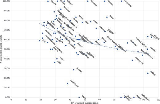
Percentage of games in which Team A achieved the desired result in the last round of year t.
Note: This figure presents the percentage of games in which Team A achieved the desired result to avoid relegation as a function of the weighted average CPI score. The detailed data are presented in Table 1 and Panel T of Table 2.
It is important to note that even if Team A won, which means that it achieved the desired result, it could still be relegated to a lower division because other teams that were likewise in danger of relegation also won their games. Panel T of Table 2 presents the detailed description of Dataset T and reveals that in the majority of the matches in the sample (61.9%), the desired result was obtained.
Detailed description of games between teams A and B
| Panel T: Games on the last day of season t between Teams A and B | |||||
|---|---|---|---|---|---|
| Team A achieved the Desired Result | |||||
| Variable Name | Yes | No | Total | Mean (rate of yes/ total) | Standard deviation |
| A has better final rank | 109 | 29 | 138 | 0.790 | 0.409 |
| B has better final rank | 403 | 286 | 689 | 0.585 | 0.493 |
| A home game | 310 | 116 | 426 | 0.728 | 0.446 |
| B home game | 202 | 199 | 401 | 0.504 | 0.501 |
| Total | 512 | 315 | 827 | 0.619 | 0.486 |
| Panel T + 1: All the last games in season t + 1 between teams A and B in which Team A achieved the desired result that in retrospect was critical in order to avoid relegation | |||||
|---|---|---|---|---|---|
| Team B won | |||||
| Variable Name | Yes | No | Total | Mean (rate of yes/ total) | Standard deviation |
| B has better final rank | 52 | 59 | 111 | 0.468 | 0.501 |
| A has better final rank | 12 | 37 | 49 | 0.245 | 0.434 |
| B home game | 39 | 40 | 79 | 0.494 | 0.503 |
| A home game | 25 | 56 | 81 | 0.309 | 0.465 |
| Total | 64 | 96 | 160 | 0.400 | 0.491 |
Note: A- Team that needs to achieve a desired result in year t to avoid relegation. B- Team that indifferent to result in year t.
In addition, according to the round-robin type of tournament used in soccer leagues, there are several rounds in which each team plays against an opponent in the pair-wise games at home and away. This structure allows us to compare games between teams A and B that were played at different stages of the tournament. Therefore, we also collected data on games between these teams that took place in previous rounds of the season. In total we have data on 1723 games. Panel T of Table 3 reveals that 47.9% of matches between teams A and B took place in the last round. This is because in most of the cases each pair competes twice a year between each other (once at its home field). In a minority of cases teams compete once, three or four times per year. We can see that in 43.8% of all games between teams A and B, Team A achieved the result that was previously classified as the desired result. More interestingly, the probability of Team A to achieve the so-called desired result in the last round was more than twice as high (61.9% versus 27.1%) compared to matches in other rounds against the same team.
Descriptive statistics
| Panel T: Dataset T—All the games between Teams A and B in the year t | |||||
|---|---|---|---|---|---|
| Variable Name | Mean | Standard deviation | Total | Min | Max |
| A achieved the Desired Result | 0.438 | 0.496 | 1723 | 0 | 1 |
| A achieved the Desired Result in the Last Round | 0.619 | 0.486 | 827 | 0 | 1 |
| A achieved the Desired Result Not in the Last Round | 0.271 | 0.445 | 896 | 0 | 1 |
| Last round | 0.480 | 0.500 | 1723 | 0 | 1 |
| CPI Score | 50.388 | 22.506 | 1723 | 15 | 99 |
| CPI*Last Round | 24.005 | 29.467 | 1723 | 0 | 99 |
| A home game | 0.503 | 0.500 | 1723 | 0 | 1 |
| Relative Rank A to B (Log2(A)-Log2(B)) | 0.975 | 1.042 | 1723 | –2.415 | 4.392 |
| Number of Clubs in the League | 15.193 | 3.538 | 1723 | 8 | 24 |
| dHHI | 0.007 | 0.005 | 1723 | 0.001 | 0.035 |
| Distance | 343.1 | 498.5 | 1721 | 0 | 5197 |
| Rule of Law Index | 0.603 | 0.193 | 1243 | 0.25 | 0.96 |
| Fisman and Miguel Index | 0.365 | 0.431 | 1584 | 0 | 1.85 |
| Log GDP per capita | 8.967 | 1.654 | 1723 | 0 | 11.631 |
| % of Protestants | 17.045 | 28.116 | 1723 | 0 | 97.8 |
| Democratic | 0.309 | 0.462 | 1723 | 0 | 1 |
| British Legal Origins | 0.211 | 0.408 | 1723 | 0 | 1 |
| Number of countries | 75 | ||||
| Panel T + 1: Dataset T + 1—Games between Team A and actual Team B and between Team A and a matched Team B in the year t + 1 | |||||
|---|---|---|---|---|---|
| Variable Name | Mean | Standard deviation | Total | Min | Max |
| A Lost | 0.423 | 0.495 | 319 | 0 | 1 |
| A Lost to Actual B | 0.400 | 0.491 | 160 | 0 | 1 |
| A lost to matched B | 0.447 | 0.499 | 159 | 0 | 1 |
| ActualB | 0.502 | 0.501 | 319 | 0 | 1 |
| CPI Score | 46.112 | 21.400 | 319 | 15 | 99 |
| CPI* ActualB | 23.106 | 27.595 | 319 | 0 | 99 |
| Relative Rank B (actual or matched) to A (Log2(B)-Log2(A)) | –0.520 | 1.160 | 319 | –4.000 | 3.585 |
| Relative Rank ActualB to A | –0.423 | 1.155 | 160 | –4.000 | 3.585 |
| Relative Rank MatchedB to A | –0.618 | 1.160 | 159 | –3.585 | 3.459 |
| TeamB (actual or matched) home game | 0.505 | 0.501 | 319 | 0 | 1 |
| ActualB home game | 0.494 | 0.502 | 160 | 0 | 1 |
| MatchedB home game | 0.516 | 0.501 | 159 | 0 | 1 |
| dHHI | 0.007 | 0.005 | 319 | 0.001 | 0.027 |
| Distance | 390.7 | 612.3 | 319 | 0 | 6836 |
| Number of countries | 58 | ||||
Note: A-Team that needs to achieve a desired result in year t to avoid relegation. B-Team that indifferent to result in year t.
Note: A-Team that needs to achieve a desired result in year t to avoid relegation. ActualB—Team that indifferent to result in year t. MatchedB—Team that finished one position above team ActualB in the year t + 1, except for seven cases in which the ActualB finished first in the league, therefore teams that finished in the second position were used as MatchedB.
2.2 Dataset T + 1—Quid pro Quo Behavior in Year t +1
Previously, Duggan and Levitt (2002) argued that in Japanese sumo matches, wrestlers tend to reciprocate. Namely, in return for getting the precious eighth victory, the winner promises to lose to his opponent in the next year. Based on this finding we investigated games in the following year (t + 1) to find out whether such reciprocation exists in soccer. For this purpose we considered all the pairs of Teams A and B in which Team A that struggled against relegation in the previous year (t), managed to achieve the desired result.
Although we are not aware of the existence of an implicit “contract of reciprocation” between the teams, there may be a difference between the cases in which Team A achieved the desired result in year t. In one case, this result was critical in retrospect for Team A. Namely, Team A would have been relegated to the lower division in the previous year without achieving this desired result. In another case, achieving the desired result was not critical in retrospect for Team A, meaning that Team A would have survived in the league even without achieving this result. This may happen because other teams that were involved in struggling against relegation were unable to achieve a result that would keep them in the league for another year. These two situations may differentially influence a team’s willingness to reciprocate in the subsequent matches against Team B in the following year. Therefore, our aim is to investigate possible quid pro quo behavior only in the pairs in which Team A avoided relegation by actually achieving the desired result in the previous year, i.e., cases in which the result in the previous year was critical in retrospect.
Consequently, we investigate Team A’s losing probability against Team B in the following year (t + 1). It is important to note that unlike sumo, where each pair of fighters competes against each other only once per season, as already stated, in the case of soccer, pairs of teams can play against each other more than once. In addition, Hill (2009) showed that there is a much higher share of fixed games in the third and fourth quadrants of the season. A possible reason for this is that the later games in the season are more important because of the fact that each game may determine the final ranking and consequently there is less time to fix mistakes. Therefore, we concentrated on the last games between the teams in the following year. In total, we analyzed 161 such games between teams A and B. However, in one case team A was dissolved in year t + 1 (Nov. Milenium from Macedonia in 2008–09 season), which leaves us with 160 observations. The last two columns of Table 1 describe the data collected for each country in the new dataset. The detailed information on this data is presented in Panel T + 1 of Table 2.
Finally, there is a possible mechanical selection of data, according to which Team A might be one of the worst teams in the league in the year t + 1, and this would be the reason that it will lose more frequently. Therefore, we use a matching approach according to which we investigate games between Team A and a team that is most similar to Team B (see, e.g., Heckman et al. (1997) for additional details on the matching approach). We took a conservative approach and collected data on all the games between Team A and a team that was ranked one position higher (better) than Team B. We used those games as a comparison group. It is important to note that there were seven cases in which an actual Team B finished first in the league, therefore teams that finished in the second position were used as matched Teams B. Finally, since one game was abandoned (CABB Arréridj versus ES Sétif in the 2008–09 season in Algeria), our database consisted of 319 games between Team A and an actual and matched Team B.
3. Variables
3.1 Variables in Dataset T
Our dependent variable, Desired ResultABit, is a dummy variable where the value 1 was assigned if the result in all the matches between teams A and B, fits the requirements of Team A (a win or in some cases a draw) in the last match against Team B in country i of year t, and zero for all other outcomes (a loss or in some cases a draw).
Since we are interested in studying the effect of countries’ corruption level on the probability of obtaining the desired result we used an index that represents the corruption level of country i during year t. One of the most common measures is the CPI published by Transparency International (TI), the global coalition against corruption. The scores range from 0 (highly corrupt) to 100 (not corrupt at all) and the scores are assigned annually to every country. When a match was played in country i in year t, the CPI score of that country in the respective year was considered.
Table 1 (except for the two last columns) describes the data collected for each country in the sample and the CPI for each country. The table shows that the CPI was almost constant over the years, with median and average standard deviations of 2.8 and 3.0, respectively.
In addition, we also consider two other measures of corrupt and/or cultural norms. The first is “Factor 2: Absence of Corruption”, obtained from the Rule of Law Index published by the World Justice Project. According to The World Justice Project (2016: 10), this factor “considers three forms of corruption: bribery, improper influence by public or private interests, and misappropriation of public funds or other resources. These three forms of corruption are examined with respect to government officers in the executive branch …, the judiciary …, the military and police …, and the legislature …, and encompass a wide range of possible situations in which corruption—from petty bribery to major kinds of fraud—can occur”.8 Similarly to the CPI score, a lower index is associated with higher corruption.
Our third measure of corrupt type of behavior was taken from Fisman and Miguel (2007), who reported parking violations per diplomat in New York in the post enforcement period between 11/2002 and 11/2005 (see Column 4 of Table 1 in Fisman and Miguel (2007)). Unlike the previous two indices, a higher number of parking violations is associated with more corrupt type of behavior.
Since our analysis focuses on the differential effect of corruption measures on the probability of attaining the desired result in the last round that was important for Team A compared to the probability of attaining a similar result in other, less decisive rounds, we created a dummy variable LastRoundABit where the value 1 was assigned if the game is played in the last round and zero otherwise. Therefore, to estimate the probability of achieving the desired result in the last game relative to a game in previous rounds and in order to compare it between different countries with regard to their corruption measures, we created an interaction between each of the corruption measures and LastRoundABit.
As already mentioned, corruption is concealed and very difficult to measure. For example, Donchev and Ujhelyi (2014) demonstrated that corruption has a significant correlation with the log (GDP) per capita; the percentage of Protestants in a country; whether a country has a solid democratic regime and British legal origins (see Column 7 of Table 4 in Donchev and Ujhelyi 2014). Therefore, we control for these variables as well in our regression analysis.
Fixed effect estimates of the effect of CPI on the probability of Team A attaining the desired result
| Dependent variable: Team A achieved the desired result | (1) | (2) | (3) | (4) | (5) | (6) | (7) |
|---|---|---|---|---|---|---|---|
| Last Round | 0.532*** | 0.516*** | 0.514*** | 0.513*** | 0.515*** | 0.408*** | 0.400*** |
| (0.057) | (0.055) | (0.055) | (0.055) | (0.055) | (0.120) | (0.119) | |
| CPI | 0.001 | 0.001 | 0.002 | 0.002 | 0.003 | 0.003 | 0.002 |
| (0.004) | (0.004) | (0.004) | (0.004) | (0.004) | (0.004) | (0.004) | |
| CPI × Last Round | –0.004*** | –0.003*** | –0.003*** | –0.003*** | –0.003*** | –0.003 | –0.003 |
| (0.001) | (0.001) | (0.001) | (0.001) | (0.001) | (0.002) | (0.002) | |
| Team A home advantage | 0.175*** | 0.177*** | 0.177*** | 0.177*** | 0.178*** | 0.177*** | |
| (0.022) | (0.022) | (0.022) | (0.022) | (0.021) | (0.021) | ||
| Log2rank(A) - Log2rank(B) | –0.107*** | –0.108*** | –0.108*** | –0.108*** | –0.108*** | ||
| (0.011) | (0.011) | (0.010) | (0.010) | (0.011) | |||
| dHHI | −13.448*** | −13.892*** | −13.914*** | −13.466*** | |||
| (4.577) | (4.646) | (4.653) | (4.587) | ||||
| Number of teams in the league | –0.000 | –0.000 | 0.000 | 0.000 | |||
| (0.008) | (0.008) | (0.008) | (0.008) | ||||
| Distance (in 1000 km) | 0.069* | 0.069* | |||||
| (0.037) | (0.037) | ||||||
| CPI × Distance (in 1000 km) | –0.001 | –0.001 | |||||
| (0.001) | (0.001) | ||||||
| logGDP × Last Round | 0.014 | 0.015 | |||||
| (0.015) | (0.015) | ||||||
| Democratic × Last Round | –0.107 | –0.108 | |||||
| (0.073) | (0.073) | ||||||
| Protestants × Last Round | 0.001 | 0.001 | |||||
| (0.001) | (0.001) | ||||||
| British Legal × Last Round | –0.030 | –0.028 | |||||
| (0.050) | (0.050) | ||||||
| Observations | 1723 | 1723 | 1723 | 1723 | 1721 | 1721 | 1723 |
| Country fixed effects | Yes | Yes | Yes | Yes | Yes | Yes | Yes |
| Year fixed effects | Yes | Yes | Yes | Yes | Yes | Yes | Yes |
| Number of Countries | 75 | 75 | 75 | 75 | 75 | 75 | 75 |
p < 0.01,
p < 0.05,
p < 0.1
Note: Standard errors clustered at the country level are in parentheses. In Column 7 we present the results of the regression that includes the union of variables selected by the two-steps LASSO variable selection. The p-val of the CPI × Last Round’s coefficient in columns 6 and 7 are 0.116 and 0.113, respectively. The bold variables are the main independent variables, in which we focus on, in each model.
The log GDP per capitait variable, is a natural log of the GDP value per capita for country i in year t.9 The percentage of Protestantsi is a variable that presents the percentage of Protestants in a particular country’s population in 1980.10 A solid democracyi is a dummy variable in which the value 1 is assigned for countries with continuous Democratic regimes for all years between 1930 through 1995.11British legal originsi is a dummy variable in which the value 1 is assigned for countries in which the legal system has British origins according to the Global Development Network Growth Database, NYU.12 Using these variables, we created interaction terms between each of them and LastRoundABit.
Since our data include both home and away games, we also control for the home advantage, which was found to be significant in previous studies (Terry et al. 1998; Garicano et al. 2005; Koning 2011). Hence, we created a dummy variable that was assigned the value of 1 if a game was played on Team A’s home field and the value of 0 if a match was played on Team B’s home field. Panel T of Table 2 shows that Team A attained the desired result in 72.8% of the home games as opposed to about 50.4% in away games.
We also control for ability differences between the teams. In line with Klaassen and Magnus (2001), we consider the final ranks of Teams A and B and add a variable that reflects the difference in rankings, calculated as . The main advantage of this measure is that the differences in team quality are not linear; instead, they grow at an increasing rate as we move up the table. This means that a difference of one position in the league’s table corresponds to a smaller difference in quality if the teams are at the bottom of the table, but corresponds to a more substantial difference when we compare top tier teams. We can see that on average, Team B is stronger than Team A as represented by a positive value of presented in Panel T of Table 3.
It is reasonable to expect that the higher ranked team has a higher probability of success. Indeed, Panel T of Table 2 shows that in 79.0% of the cases in which Team A was ranked higher than Team B, Team A attained the desired result. However, when Team B had a better final rank than Team A, then only in about 58.5% of the cases did Team A attain the desired result.
3.2 Variables in Dataset T + 1
In this dataset, our dependent variable is , which is a dummy variable where the value of 1 is assigned if Team A lost the game in the following year (t + 1) to Team B or matched Team B and the value of zero is assigned for all other outcomes. For reasons discussed above, we are interested in the last game of the following season between Team A and Team B and between Team A and matched Team B.
As already mentioned, Team A might have a different sense of obligation toward Team B in cases when the result of the game in the previous year was critical for Team A in retrospect as opposed to cases when it was not critical for Team A in retrospect. Namely, when Team A would have been relegated to the lower division in the previous year without achieving this desired result, as opposed to cases when achieving the desired result was not critical in retrospect for Team A. The latter case implies that Team A would have survived in the league even without achieving the desired result. In total we have 161 matches from 57 different countries between Team A and Team B, where obtaining the desired result was retrospectively critical for Team A. Panel T + 1 of Table 2 shows that Team B won in 40% of those matches.
For this dataset, our analysis focuses on the differential effect of the CPI on the probability of Team A losing against Team B compared to the probability of losing against matched Team B. For this, we created a dummy variable ActualBABit+1 where the value 1 is assigned if Team A competes against actual Team B and zero if it competes against a matched Team B. To estimate the probability of losing to actual Team B compared to the odds of losing against a matched Team B and in order to compare it between different countries with regard to their CPI score, we created an interaction between the CPI and ActualBABit+1.
Panel T + 1 of Table 3 reveals that the difference in rankings between an actual Team B and Team A is lower than the difference in rankings between a matched Team B and Team A. In other words, this implies that on average, the matched Team B is stronger than the actual Team B. This is not surprising, since in all, but seven cases, we defined a matched Team B as a team that finished in a better position than the actual Team B.
As previously, we also control for the home advantage, the differences in ability between the teams and the competitive balance of the league. Therefore, we created a dummy variable assigned the value of 1 if the match was played at (actual or matched) Team B’s home field and the value of zero if the match was played at Team A’s home field. The ability differences measure between actual or matched Team B and Team A was defined as log2(Rank of Team B)–log2(Rank of Team A). The last control variable is the league according to the final table of year t + 1.
4. Empirical Evidence
4.1 Main Results for Year t
This specification allows us to compare the probability of attaining the desired result in more corrupt countries relative to less corrupt countries in the last round, when the game is important for Team A versus other rounds. In other words, the interaction coefficient between and measures the differential effect of CPI between playing in the last, most decisive round, and other rounds. A negative value of implies that in more corrupt countries (lower CPI), there is a higher probability that Team A achieves the desired result in the last round relative to other rounds. In addition, it is plausible to assume that our setting does not suffer from possible reverse causality as may appear in relationships between the corruption index and different economic measures (Treisman 2000). This is because, the performance of soccer players is unlikely to affect the corruption index; it is rather the other way around, that a corrupt environment affects the results of the soccer games.
Column 1 of Table 4 presents the results from estimating equation (1) without a list of basic controls, where standard errors clustered at the country level are in the parentheses. The results show that the coefficient of the interaction term, , is negative and significant at the 1% level. This implies that Team A has a significantly higher probability of attaining the desired result in more corrupt countries in the last round, when the game is the most important for Team A, relative to other rounds. This result implies that one standard deviation increase (29.5 CPI points) in the interaction term between a dummy variable and the is associated with a decreased probability of Team A to achieve the desired result by about 11.8 percentage points on average, which is about 25% of the sample mean (the mean value of Team A to achieve the desired result is 43.8%).
We can see that the results are not sensitive to the set of controls, such as the home advantage, difference in rankings and the competitive balance of the league as presented in Columns 2–4. One possible concern, however, is that familiarity between the clubs as expressed by a smaller distance between the cities may drive our results. Therefore, in Column 5, we also control for distance between the cities and interaction between the distance and the CPI. We can see that the interaction coefficient is robust to inclusion of these controls as well.
As discussed previously, the corruption variable is based on subjective surveys. It was previously found that the CPI is highly correlated with several other variables related to a country such as log of GDP per capita, the percentage of Protestants in the population, democratic solidity of its government, and its grounding in British legal origins. Therefore, our results may be driven by other social aspects that are highly correlated with the CPI and not by the CPI itself. Hence, in Column 6 we also control for the interaction of each of the closely related to CPI variables and the . Not surprisingly, we find that none of the interactions are significant. This is because each of them is reflected in the CPI, and, therefore, we expect a bias of the results toward zero when controlling for these variables. As Belloni et al. (2014) asserted: “We are faced with a tradeoff between controlling for very few variables which may leave us wondering whether we have included sufficient controls for the exogeneity of the treatment and controlling for so many variables that we are essentially mechanically unable to learn about the effect of the treatment” (p. 638). Nevertheless, even after controlling for so many endogenous variables, the coefficient of our interest is very close to significant levels with p-val = 0.116. In fact, it is the most significant coefficient out of all interactions with the .
In Column 7 we follow the approach proposed by Belloni et al. (2014) and use two LASSO (Least Absolute Shrinkage and Selection Operator) estimations for variables selection. In the first step we select a set of control variables that are useful for predicting the . In the second step we select additional variables by selecting control variables that predict our outcome, namely whether or not Team A achieved the desired result. In the final step we estimate the effect of by including the union of variables that were selected in the first two steps. The only two variables that are not countries and years dummies that were not selected are distance related variables. However, not surprisingly, all the variables that are strongly associated with the CPI were selected in the first step and therefore the results in Column 7 are very similar to those presented in Column 6, where has the p-val of 0.113.14 In the following sub-section we show that the effect of corruption as measured by the CPI on the probability to attain the desired result comes from the most corrupt countries, and that this effect is significant even when controlling for all variables correlated with the CPI.
4.2 Quartile Approach
Previous studies found biases in reported perceptions (Olken 2009; Beaman et al. 2009; Campbell 2013). In this sub-section we intend to examine whether the relationship between the CPI and the probability of attaining the desired result is continuous throughout the scale of scores. For this purpose, we created four dummy variables with the same number of observations. The first dummy variable (Q1) is assigned a value of 1 if the CPI score is in the lower quartile of the observations (most corrupt countries with CPI less than 30); the second (Q2) is assigned a value of 1 if it is between one quarter and one half of the observations (CPI scores in the range of 30–43); the third (Q3) if it is between one half and three quarters of the observations (CPI scores in the range of 44–64); and the fourth (Q4) if it is higher than three quarters (scores of 65 and above). Then we interact these variables with . To avoid multicollinearity, we omit the first category and use it as a reference category.
The results, presented in Table 5, are consistent with our previous results. We can see that the coefficients of the third and the fourth quartiles are negative and the size of the coefficient decreases with the CPI score. In addition, the coefficient of is always significant. This implies that relative to the most corrupt countries according to the CPI score, which are represented in Q1, the probability of Team A to attain the desired result in the last round relative to the previous rounds is significantly lower. The estimated effect is about 19.5 percentage points. Moreover, when we control jointly for all variables correlated with the CPI (see Column 4), then in most transparent countries (Q4), according to the CPI, the probability for Team A to achieve the desired result in the last round relative to other rounds is significantly lower than in more corrupt countries. Furthermore, none of the variables correlated with the CPI remain significant.
Fixed effect estimates of the effect of CPI’s quartile on the probability of Team A attaining the desired result
| Dependent variable: Team A achieved the desired result | (1) | (2) | (3) | (4) |
|---|---|---|---|---|
| Last Round | 0.407*** | 0.403*** | 0.403*** | 0.294** |
| (0.041) | (0.041) | (0.042) | (0.121) | |
| Q2 × Last Round | 0.043 | 0.032 | 0.033 | 0.032 |
| (0.051) | (0.048) | (0.048) | (0.052) | |
| Q3 × Last Round | –0.064 | –0.071 | –0.068 | –0.076 |
| (0.063) | (0.063) | (0.063) | (0.075) | |
| Q4 × Last Round | −0.206*** | −0.194*** | −0.194*** | –0.200* |
| (0.065) | (0.065) | (0.065) | (0.108) | |
| logGDP × Last Round | 0.015 | |||
| (0.015) | ||||
| Democratic × Last Round | –0.080 | |||
| (0.076) | ||||
| Protestants × Last Round | 0.001 | |||
| (0.001) | ||||
| British Legal × Last Round | –0.043 | |||
| (0.053) | ||||
| Test of Q2–Q3 = 0 (p-val) | 0.068 | 0.061 | 0.068 | 0.072 |
| Test of Q2–Q4 =0 (p-val) | 0.000 | 0.000 | 0.000 | 0.013 |
| Test of Q3–Q4 = 0 (p-val) | 0.022 | 0.048 | 0.044 | 0.149 |
| Observations | 1723 | 1723 | 1721 | 1721 |
| Country fixed effects | Yes | Yes | Yes | Yes |
| Basic controls | No | Yes | Yes | Yes |
| Distance controls | No | No | Yes | Yes |
| Year fixed effects | Yes | Yes | Yes | Yes |
| Number of Countries | 75 | 75 | 75 | 75 |
p < 0.01,
p < 0.05,
p < 0.1
Note: Standard errors clustered at the country level are in parentheses. Our list of basic controls includes the Team A home advantage, Log2rank(A) - Log2rank(B), dHHI and number of teams in the league. Distance controls include distance in 1000 km between the cities of the teams and the interaction between this distance and the CPI.
In addition, in all the cases, is positive and not significant. This implies that there is no meaningful difference between the first and the second quartiles in terms of the prospects of Team A to achieve the desired result in the last round relative to the previous rounds. Our results suggest that the effect of corruption is non-linear. For example, Salmon and Serra (2017) found that a possibility of social judgment reduces corruption only among individuals who identify culturally with countries below a certain threshold (USA corruption index). It is possible that there is some threshold below which there is no significant difference in corrupt norms of the participants. In our case, in the bottom half of the CPI score they behave in a similar and corrupt way. However, as we climb the CPI scale, the differences between the countries become more conspicuous, and the values of transparency become more important. As evidence, we found that is significantly different from in all the cases and significantly different from in all the cases except for the last column. As well, we found that is significantly different from in all the cases (see p-val for these tests reported in Table 5).
4.3 Other Measures of Corrupt Behavior
One may be concerned that, for whatever reason, the CPI index does not represent corrupt types of behavior, but rather other traits that are correlated with it. Therefore, we conducted the same analysis as presented in Table 4, but with two other measures that also intend to represent corrupt norms. The first is “Factor 2: Absence of Corruption”, obtained from the 2016 Rule of Law Index published by the World Justice Project. And the second is parking violations per diplomat in the period between 11/2002 and 11/2005, obtained from Column 4 of Table 1 in Fisman and Miguel (2007).
In Columns 1–3 of Table 6, we present the results for the “Factor 2: Absence of Corruption” as a corruption index, whereas in Columns 4–6, similar analysis is conducted for the parking violations as a measure of corrupt type of behavior. We can see that in all the cases, the interaction of the corruption index with is significant and with the correct sign (negative for “Factor 2: Absence of Corruption” and positive for the parking violations). These results imply that our findings are robust to different measures of corruption.
Fixed effect estimates of the effect of other corruption related measures on the probability of Team A attaining the desired result
| Dependent variable: Team A achieved the desired result | (1) | (2) | (3) | (4) | (5) | (6) |
|---|---|---|---|---|---|---|
| Last Round | 0.597*** | 0.556*** | 0.556*** | 0.361*** | 0.301*** | 0.301*** |
| (0.083) | (0.080) | (0.080) | (0.030) | (0.029) | (0.029) | |
| Rule Law × Last Round | –0.367** | –0.301** | –0.301** | |||
| (0.142) | (0.137) | (0.137) | ||||
| Fisman and Miguel × Last Round | 0.141*** | 0.117*** | 0.121*** | |||
| (0.034) | (0.037) | (0.036) | ||||
| Observations | 1243 | 1243 | 1243 | 1584 | 1584 | 1582 |
| Country fixed effects | Yes | Yes | Yes | Yes | Yes | Yes |
| Basic Controls | No | Yes | Yes | No | Yes | Yes |
| Distance controls | No | No | Yes | No | No | Yes |
| Year fixed effects | Yes | Yes | Yes | Yes | Yes | Yes |
| Number of Countries | 49 | 49 | 49 | 68 | 68 | 68 |
p < 0.01,
p < 0.05,
p < 0.1
Note: Standard errors clustered at the country level are in parentheses. Our list of basic controls includes the Team A home advantage, Log2rank(A)–Log2rank(B), dHHI and number of teams in the league. Distance controls include distance in 1000 km between the cities of the teams and the interaction between this distance and each of the measures of corrupt norms in the respective analysis. The bold variables are the main independent variables, in which we focus on, in each model.
4.4 Quid pro Quo Behavior
In previous sub-sections, we found that in more corrupt countries according to the CPI, there is a higher probability that Team A will achieve the desired result against Team B in the most decisive, last round, relative to other, less decisive rounds. Based on Duggan and Levitt’s (2002) finding on reciprocation, our aim in this sub-section is to investigate matches in the following year (t + 1) to find out whether such quid pro quo behavior, which may be treated as a type of corruption, exists in soccer.
For this test, we limited the database to 160 observations in which the result of the game in the last day of the season in year t was critical for Team A in retrospect. In other words, we only analyze pairs in which Team A avoided relegation by actually achieving the desired result in the previous year; that is, cases in which the result in the previous year was critical in retrospect.
Figure 2 plots the percentage of times in which Team A lost to Team B in their last meeting of the following year t + 1 as a function of the country’s weighted average CPI score that is shown in Table 1. We can see that the higher the CPI score, the lower is the probability that Team A loses in the following year.
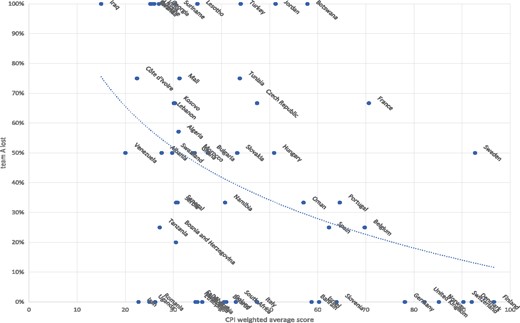
Percentage of games in which Team B won in the last match against Team A in the following year (t + 1).
Note: This figure presents the percentage of games in which Team A lost to the actual Team B in the year t + 1, one year after Team A achieved the desired result that in retrospect was critical to avoid relegation. The detailed data are presented in Table 1 and Panel T + 1 of Table 2.
This specification allows us to compare the probability that Team A loses more often in more corrupt countries (lower CPI) to the actual Team B (), than to the matched Team B compared to less corrupt countries (higher CPI). Such an outcome will be represented by a negative value of . Indeed, as presented in Table 7, the coefficient of the interaction between and is negative and significant at the 10% level, implying that in more corrupt countries according to the CPI, Team A loses more often to the actual Team B, than to the matched Team B.15 This result implies that one standard deviation increase (27.6 CPI points) in the interaction term between and is associated with a decreased probability of Team A losing to the actual Team B compared to the matched Team B by about 11 percentage points. Similar to the results presented in Table 4, it is about 25% of the sample mean (the mean value of Team A to lose against an actual or matched Team B is 42.3%).
Fixed effect estimates of the CPI on the probability of Team A to lose against Team B in the following year
| Dependent variable: Team A lost | (1) | (2) | (3) | (4) | (5) |
|---|---|---|---|---|---|
| ActualB | 0.156 | 0.155 | 0.155 | 0.177 | 0.173 |
| (0.143) | (0.134) | (0.135) | (0.135) | (0.137) | |
| CPI | –0.016 | –0.012 | –0.011 | –0.010 | –0.010 |
| (0.013) | (0.013) | (0.013) | (0.012) | (0.013) | |
| CPI*ActualB | –0.004* | –0.004* | –0.004* | –0.004* | –0.004* |
| (0.002) | (0.002) | (0.002) | (0.002) | (0.002) | |
| Team B home advantage | 0.277*** | 0.278*** | 0.266*** | 0.265*** | |
| (0.061) | (0.061) | (0.058) | (0.059) | ||
| dHHI | –2.906 | –9.086 | –9.447 | ||
| (9.702) | (10.081) | (10.139) | |||
| Relative Rank B to A (Log2(B)-Log2(A)) | –0.139*** | –0.141*** | |||
| (0.031) | (0.032) | ||||
| Distance (in 1000 km) | 0.015 | ||||
| (0.211) | |||||
| CPI*Distance (in 1000 km) | –0.001 | ||||
| (0.004) | |||||
| Observations | 319 | 319 | 319 | 319 | 319 |
| Country fixed effects | Yes | Yes | Yes | Yes | Yes |
| Year fixed effects | Yes | Yes | Yes | Yes | Yes |
| Number of Countries | 58 | 58 | 58 | 58 | 58 |
p < 0.01,
p < 0.05,
p < 0.1
Note: Standard errors clustered at the country level are in parentheses. The bold variables are the main independent variables, in which we focus on, in each model.
The finding that in more corrupt countries, Team A loses more often to a weaker team than to a better team strongly supports the interpretation that the results of our study are driven by corrupt norms, rather than by any other explanation.
5. Conclusion
This article was inspired by two studies. The first is the cross-country analysis of a real-life rule breaking experiment conducted by Fisman and Miguel (2007) who found a positive relationship between diplomatic parking violations and corruption measures in diplomats’ home countries, concluding that cultural norms are important determinants of corruption. Our aim was to provide a test of external validity regarding the results of Fisman and Miguel (2007) by using different types of participants in a different real-life situation that may provoke a corrupt type of behavior.
The second study that inspired us was the study of Duggan and Levitt (2002) on the relationship between sharp non-linearity in the payoff functions of the agents and corrupt behavior in sumo. A similar situation that provokes a rule-breaking behavior occurs in sensitive soccer games. In these games one of the teams (Team A) had to achieve a desired result on the last day of the season in order to avoid relegation to a lower division, while the other team (Team B) was not affected by the result of the respective game. Based on this similar situation in 75 different countries during the period between 2001 through 2013 our findings indicate that the likelihood that Team A attains such a result in the most decisive games is significantly higher than in less important matches against the same Team B when a country is more corrupt. We also find strong evidence of a significant association between the corruption index and the quid pro quo behavior that raises serious questions about possible illegal activities that could have taken place in the matches that involved teams A and B.
Our results suggest that despite the fact that all the participants compete under fixed and known rules that were determined by the soccer governing body, International Federation of Association Football (FIFA), and despite the fact that all teams face the exact same incentives regarding the possible relegation to a lower division, the prevalence of corruption in the institutional environment where the games take place seems to shape behavior.
Finally, it is clear that a more effective fight against corruption requires a better understanding of its mechanisms. Therefore, anti-corruption reform makers should identify settings that may provoke corrupt types of behavior and find alternative settings that serve the same goal but with a lower possibility for rule-breaking behavior. In the specific case of soccer, it would be helpful if all the games were important to both teams. For example, in the playoff structure, where two teams compete against each other and a loser is eliminated, there is no sharp non-linearity in the payoff functions, which might reduce the willingness for quid pro quo arrangements.
Guy Elaad and Alex Krumer equally contributed to this article, which is a substantially revised version of “Does Corruption Perceptions Index Predict the Outcome of Competition? Evidence from a Natural Experiment around the World” and “Corruption and Contests: Cross-Country Evidence from Sensitive Soccer Matches”. We would like to thank Bernd Frick, Daniele Paserman, Danny Cohen-Zada, Ignacio Palacios-Huerta, Mark Gradstein, Michael Knaus, Michael Lechner, Moshe Justman, Offer Moshe Shapir, Roland Hodler, Ruud Koning, Stefan Szymanski, seminars and conferences participants at Ben Gurion University of the Negev, University of St. Gallen, Bar Ilan University, University of Groningen, NYU Shanghai, the 7th conference of the European Sports Economics Association, and the 31st annual congress of the European Economic Association as well as editor and two anonymous referees for their helpful comments and suggestions. All errors are our own.
Appendix A
List of Sources
Appendix B
List of countries sampled by division
| 1st Division Countries | 2nd Division Countries |
|---|---|
| Albania | Austria |
| Algeria | Belarus |
| Azerbaijan | Belgium |
| Bahrain | Bosnia and Herzegovina |
| Botswana | Bulgaria |
| Côte d´Ivoire | Czech Republic |
| Djibouti | Denmark |
| Ethiopia | England as UK representative |
| Gabon | Estonia |
| Georgia | Finland |
| Ghana | France |
| Guatemala | Germany |
| Guinea | Greece |
| Hong Kong | Hungary |
| India | Iceland |
| Iran | Ireland |
| Iraq | Israel |
| Jordan | Italy |
| Kosovo | Latvia |
| Kuwait | Macedonia |
| Lebanon | Netherlands |
| Lesotho | Norway |
| Luxembourg | Poland |
| Mali | Portugal |
| Mauritania | Romania |
| Mauritius | Russia |
| Morocco | Serbia |
| Namibia | Slovakia |
| Oman | Slovenia |
| Qatar | Spain |
| Rwanda | Sweden |
| Saudi Arabia | Switzerland |
| Senegal | Turkey |
| South Africa | Ukraine |
| Suriname | |
| Swaziland | |
| Tanzania | |
| Tunisia | |
| Uganda | |
| United Arab Emirates | |
| Venezuela |
Footnotes
1. See also Armantier and Boly (2013) who compared corruption in laboratory and field experiments run in Canada and Burkina Faso.
2. According to the US Supreme Court in Buckley v. Valeo, 424 U.S. 1 (1976:27): “Of almost equal concern as the danger of actual quid pro quo arrangements is the impact of the appearance of corruption …”. See also Lambsdorff and Frank (2010) who studied quid pro quo in experimental settings.
3. The association between soccer and corruption has already been recognized. Hill (2010) exposed several potentially explosive stories of match-fixing in professional soccer, from domestic professional soccer leagues to games that were fixed in the 2006 International Federation of Association Football (FIFA) World Cup. See also McLaren (2008) and Preston and Szymanski (2003) for additional examples of corruption in sports.
4. Miguel et al. (2008) were the first to use soccer games to explore cross-country cultural norms regarding violence. They investigated the relationship between the history of civil conflict in a player’s home country and his propensity to behave violently on the soccer field.
5. According to soccer governing body’s (FIFA) Rule 1 of the code of conduct “winning is the object of playing any game”. From http://www.fifa.com/about-fifa/news/y=2002/m=4/news=code-conduct-for-football-81746.html. Last accessed on 26 March 2018.
6. The Corruption Perceptions Index is published by Transparency International (TI), the global coalition against corruption. For example, for 2013, 13 data sources were used to construct the CPI of countries: African Development Bank Governance Ratings 2012; Bertelsmann Foundation Sustainable Governance Indicators 2014; Bertelsmann Foundation Transformation Index 2014; Economist Intelligence Unit Country Risk Ratings; Freedom House Nations in Transit 2013; Global Insight Country Risk Ratings; International Institute for Management Development (IMD) World Competitiveness Yearbook 2013; Political and Economic Risk Consultancy Asian Intelligence 2013; Political Risk Services International Country Risk Guide; Transparency International Bribe Payers Survey 2011; World Bank—Country Policy and Institutional Assessment 2012; World Economic Forum Executive Opinion Survey (EOS) 2013 and World Justice Project Rule of Law Index 2013.
7. There is anecdotal evidence of possible existence of quid pro quo in Russia after the resignation of the coach of Ural Yekaterinburg, Victor Goncharenko, before the match against Terek Grozny in September 2015. According to Russian press, the result of this match was suspected as being fixed. From: https://sport.rbc.ru/news/5754b1b69a7947133b2970e0 (in Russian). The official reason for resignation was “divergence in views on the further development of the club”. More interestingly, in the last round of the antecedent season, Terek, which can be referred as Team B lost at home to Ural (Team A), which helped the latter to avoid relegation. The resignation of Goncharenko was followed by heated debates on whether the match was fixed or not. The final score of this match was 3:3. However, one year later, Terek won 4:1 in Yekatirenburg. Following this match, one of the leading Russian sport reporters, Vasily Utkin published an article where he called the result of this match fixed. From: https://www.sports.ru/tribuna/blogs/odukhevremeni/1096345.html (in Russian). The links were last accessed on 9 March 2018.
8. We consider the 2016 edition of the index, since it contains the largest number of countries. From: https://worldjusticeproject.org/sites/default/files/documents/RoLI_Final-Digital_0.pdf. Last accessed on 21 April 2017.
9. Taken from the “GDP per capita (current US$)” indicator of the World Bank Database.
10. According to La Porta et al. (1999) the data on this variable was downloaded from the Quality of Government Database at the Quality of Government Institute at Gothenburg University.
11. According to the classification by Beck et al. (2001), democracies are those with a score of 6 or higher on the Executive Index of Electoral Competitiveness (EIEC).
12. The percentage of Protestants, data on democracies and data on whether or not the legal origins were British were drawn from the Treisman (2007) database.
13. The distance was obtained from www.maps.google.com.
14. As part of the identification strategy where we use countries and years fixed effects we did not drop the unselected countries and years. Dropping these unselected dummies does not significantly change the results. The results of this regression are available upon request.
15. The analysis that includes interactions between and all correlated with the CPI variables yields insignificant results for all interactions, which is not surprising given the multicollinearity problem as well as the significantly lower number of observations relative to Dataset T. The results are available upon request.
