


Abstract
Pricklebacks (Family Stichaeidae) are generally cold-temperate fishes most commonly found in the north Pacific. As part of the California Conservation Genomics Project (CCGP), we sequenced the genome of the Monkeyface Prickleback, Cebidichthys violaceus, to establish a genomic model for understanding phylogeographic patterns of marine organisms in California. These patterns, in turn, may inform the design of marine protected areas using dispersal models based on forthcoming population genomic data. The genome of C. violaceus is typical of many marine fishes at less than 1 Gb (genome size = 575.6 Mb), and our assembly is near-chromosome level (contig N50 = 1 Mb, scaffold N50 = 16.4 Mb, BUSCO completeness = 93.2%). Within the context of the CCGP, the genome will be used as a reference for future whole genome resequencing projects, enhancing our knowledge of the population structure of the species and more generally, the efficacy of marine protected areas as a primary conservation tool across California’s marine ecosystems.
Introduction
The Monkeyface Prickleback, like most marine fishes, exhibits a biphasic life history, with a vagile pelagic larval stage followed by a more sedentary post-metamorphic stage (Leis 1991). Dispersal potential in coastal marine fishes is affected by method of fertilization (internal vs. external), egg type (internal, deposited on the substrate, or pelagic), and larval behavior (swimming or passive). In California, pricklebacks (Family Stichaeidae) are oviparous and deposit their eggs on rocky surfaces where nest guarding has been observed, but it is unclear whether the males, females, or both guard the brood until hatching (Love 2011). Larval duration after hatching and the level of genetic structure across the species’ range is presently unknown.
There are 17 species of prickleback in 13 genera that occur in California. Cebidichthys violaceus is the only representative of the genus and is nestled within a clade including Esslenichthys and Dictyosoma, the latter of which is found in the Western Pacific (German et al. 2014; Kim et al. 2014) (Fig. 1). Other stichaeid species commonly found in the rocky intertidal zone of California include the genera Anoplarchus, Esselenichthys, Phytichthys, and Xiphister (German et al. 2014; Kim et al. 2014). Cebidichthys, along with Xiphister mucosus, are primarily herbivores as adults. In its early life stages, C. violaceus primarily consumes zooplankton. At a body length of ~7 cm the species transitions to a diet consisting primarily of red and green algae (Setran and Behrens 1993).
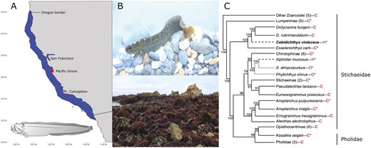
A) Distribution of Monkeyface Prickleback, Cebidichthys violaceus. Monkeyface Pricklebacks are found in the intertidal and subtidal to a depth of 25 m from Southern Oregon, USA, to Northern Baja California, Mexico. The collection site of the sequenced individual, Pacific Grove California, is indicated by the star on the map. Inset is an illustration of C. violaceus (Illustration credit: Andrea Dingeldin). B) A Monkeyface Prickleback, C. violaceus (photo by M.H. Horn) and an image of Franklin Point California at low tide, an example of representative intertidal habitat for the Monkeyface Prickleback. C) Phylogenetic relationships of the nonmonophyletic family Stichaeidae based on 2,100 bp of cytb, 16s, and tomo4c4 genes (Kim et al. 2014). Bayesian posterior probabilities are indicated on nodes. C. violaceus is bolded and the letters after the names are H = herbivory, O = omnivory, C = carnivory. Evolution of herbivory (— — — —) and omnivory (............) are shown. Numbers in parentheses are the number of taxa contained in that branch. Some groups are collapsed into subfamilies. Asterisks indicate that this species (or species in that group) are found in California.
Monkeyface Pricklebacks can attain a total length of 76 cm, moving from the high intertidal to the shallow subtidal as they grow. They are relatively long lived (19 yr) and slow growing, reaching sexual maturity between 4 and 7 yr of age at a body length of 36 to 45 cm (Love 2011). The species ranges from Southern Oregon to Northern Baja California, MX (Fig. 1), though they are rarely reported south of Point Conception, Santa Barbara County, California. They are the target of a small but dedicated recreational fishery that uses leaders attached to a bamboo shoot to present bait into the caves and crevices that C. violaceus inhabits, a practice known as “poke poling” (Leet 2001). The species also supports a small commercial fishery, and it is common to find Monkeyface Prickleback as a menu item in Northern California and Oregon restaurants. More recently, given its herbivorous diet, C. violaceus has been identified as a candidate for aquaculture to meet the demand for marine protein using sustainable, plant-based aquaculture feeds. Previous genomic and biochemical work on C. violaceus suggests that it can digest the lipids in plant-based feed pellet (Heras et al. 2020), unlike the more typical carnivorous aquaculture species (e.g. rainbow trout; Sahaka et al. 2020). To date, no phylogeographic or population genetic work has been published on the species.
As a result of their unusual life history traits, intertidal species exhibit low levels of dispersal, resulting in a high potential for local adaptation and strong within-species phylogeographic structure (Hickerson and Cunningham 2005; Johnson et al. 2016). Given this, pricklebacks may serve as a predictive model species of phylogeographic breaks along the California coast that contributes to optimizing the design and boundaries of marine conservation priorities targeting low-vagility taxa. To further this important goal, which is one of the key marine objectives of the California Conservation Genomics Project (CCGP), we sequenced and assembled a reference genome for the Monkeyface Prickleback, C. violaceus, following the overall CCGP framework (Shaffer et al. 2022).
The assembled genome of C. violaceus described here will serve as a valuable resource for studying the ecology, life history, adaptation, dispersal capability, and distribution dynamics of this ecologically and recreationally important species, as well as establish a useful model species for the study of evolutionary dynamics along the California Current Large Marine Ecosystem (CCLME).
Methods
Biological materials
One adult Monkeyface Prickleback, C. violaceus, was collected by dip net at low tide near Pacific Grove California (N 36.6355 W −121.9255) in September 2020 by the senior author under California Department of Fish and Wildlife permit GM-201270003-20134-001 (Fig. 1). The fish was brought live to the lab, euthanized, and liver, muscle, fin and gill tissues were dissected and immediately flash frozen in liquid nitrogen. Samples were later transferred to a −80 °C freezer until DNA extraction.
High molecular weight genomic DNA isolation
High molecular weight (HMW) genomic DNA (gDNA) was extracted from 39 mg of fin tissue using the Nanobind Tissue Big DNA kit (Pacific Biosciences—PacBio, CA) following manufacturer’s instructions. Purity of gDNA was accessed using a NanoDrop ND-1000 spectrophotometer and 260/280 ratio of 1.82 and 260/230 of 2.94 were observed. DNA yield (11 µg total) was quantified using Qbit 2.0 Fluorometer (Thermo Fisher Scientific, MA). Integrity of the HMW gDNA was verified on a Femto pulse system (Agilent Technologies, CA) where 75% of the DNA was found in fragments above 50 kb and 65% of DNA was found in fragments above 100 kb.
HiFi library preparation and sequencing
The HiFi SMRTbell library was constructed using the SMRTbell Express Template Prep Kit v2.0 (PacBio, Cat. #100-938-900) according to the manufacturer’s instructions. HMW gDNA was sheared to a target DNA size distribution between 15 and 20 kb. The sheared gDNA was concentrated using 0.45× of AMPure PB beads (PacBio Cat. #100-265-900) for the removal of single-strand overhangs at 37 °C for 15 min, followed by further enzymatic steps of DNA damage repair at 37 °C for 30 min, end repair and A-tailing at 20 °C for 10 min and 65 °C for 30 min, ligation of overhang adapter v3 at 20 °C for 60 min and 65 °C for 10 min to inactivate the ligase, then nuclease treated at 37 °C for 60 min. The SMRTbell library was purified and concentrated with 0.45× Ampure PB beads (PacBio, Cat. #100-265-900) for size selection using the BluePippin/PippinHT system (Sage Science, MA; Cat #BLF7510/HPE7510) to collect fragments greater than 7 to 9 kb. The 15 to 20 kb average HiFi SMRTbell library was sequenced at University of California Davis DNA Technologies Core (Davis, CA) using one 8M SMRT cell, Sequel II sequencing chemistry 2.0, and 30-h movies each on a PacBio Sequel II sequencer.
Omni-C library preparation
The Omni-C library was prepared using the Dovetail Omni-C Kit (Dovetail Genomics, CA) according to the manufacturer’s protocol with slight modifications. First, specimen tissue was thoroughly ground with a mortar and pestle while cooled with liquid nitrogen. Subsequently, chromatin was fixed in place in the nucleus, and the suspended chromatin solution was passed through 100 and 40 µm cell strainers to remove large debris. Fixed chromatin was digested under various conditions of DNase I until a suitable fragment length distribution of DNA molecules was obtained. Chromatin ends were repaired and ligated to a biotinylated bridge adapter followed by proximity ligation of adapter-containing ends. After proximity ligation, crosslinks were reversed, and the DNA was purified from proteins. Purified DNA was treated to remove biotin that was not internal to ligated fragments, and a NGS library was generated using an NEB Ultra II DNA Library Prep kit (New England Biolabs, MA) with an Illumina compatible y-adaptor. Biotin-containing fragments were then captured using streptavidin beads prior to PCR enrichment. The library was sequenced at Vincent J. Coates Genomics Sequencing Lab (Berkeley, CA) on an Illumina NovaSeq (Illumina, CA) platform to generate approximately 100 million 2 × 150 bp read pairs per GB genome size.
Nuclear genome assembly
We assembled the genome of the Monkeyface Prickleback following the CCGP assembly protocol Version 3.0, which uses PacBio HiFi reads and Omni-C data to generate high quality and highly contiguous genome assemblies (see Table 1). Briefly, we removed remnant adapter sequences from the PacBio HiFi dataset using HiFiAdapterFilt (Sim et al. 2022) and generated an initial diploid assembly with the filtered PacBio reads using HiFiasm (Cheng et al. 2021). The diploid assembly consists of 2 pseudo haplotypes (primary and alternate), where the primary assembly is more complete and consists of longer phased blocks, and the alternate consists of haplotigs (contigs with the same haplotype) in heterozygous regions and is not as complete and more fragmented. Given the characteristics of the latter, it cannot be considered on its own but as a complement of the primary assembly (https://lh3.github.io/2021/04/17/concepts-in-phased-assemblies, https://www.ncbi.nlm.nih.gov/grc/help/definitions/).
Assembly pipeline and software used.
| Assembly | Software and optionsa | Version |
|---|---|---|
| Filtering PacBio HiFi adapters | HiFiAdapterFilt | Commit 64d1c7b |
| K-mer counting | Meryl | 1 |
| Estimation of genome size and heterozygosity | GenomeScope HiFiasm (Hi-C mode, –primary, p_ctg, and a_ctg output) | 2 |
| De novo assembly (contiging) | 0.16.1-r375 | |
| Remove low-coverage, duplicated contigs | purge_dups | 1.2.6 |
| Scaffolding | ||
| Omni-C scaffolding | SALSA (-DNASE, -i 20, -p yes) | 2 |
| Gap closing | YAGCloser (-mins 2 -f 20 -mcc 2 -prt 0.25 -eft 0.2 -pld 0.2) | Commit 20e2769 |
| Omni-C contact map generation | ||
| Short-read alignment | BWA-MEM (-5SP) | 0.7.17-r1188 |
| SAM/BAM processing | samtools | 1.11 |
| SAM/BAM filtering | pairtools | 0.3.0 |
| Pairs indexing | pairix | 0.3.7 |
| Matrix generation | cooler | 0.8.10 |
| Matrix balancing | HicExplorer (hicCorrectmatrix correct -- filterThreshold -2 4) | 3.6 |
| HiGlass | 2.1.11 | |
| PretextMap | 0.1.4 | |
| PretextView | 0.1.5 | |
| Contact map visualization | PretextSnapshot | 0.03 |
| Organelle assembly | ||
| Mitogenome assembly | MitoHiFi (-r, -p 50, -o 1) | Commit c06ed3e |
| Genome quality assessment | ||
| Basic assembly metrics | QUAST (--est-ref-size) | 5.0.2 |
| BUSCO (-m geno, -l actinopterygii) | 5.0.0 | |
| Merqury | 2022-01-29 | |
| Assembly completeness | Repeat Masker (-s, “actinopterygii”) | 4.1.2-p1 |
| Contamination screening | ||
| General contamination screening | BlobToolKit | 2.3.3 |
| Local sequence alignment | BLAST+ | 2.1 |
Software citations are listed in the text.
aOptions detailed for nondefault parameters.
Next, we identified sequences corresponding to haplotypic duplications and contig overlaps on the primary assembly with purge_dups (Guan et al. 2020), transferred them to the alternate assembly, and scaffolded both assemblies using the Omni-C data with SALSA (Ghurye et al. 2019).
The primary assembly was manually curated by generating and analyzing Omni-C contact maps and breaking the assembly where major misassemblies were found. No further joins were made after this step. To generate the contact maps, we aligned the Omni-C data against the corresponding reference with BWA-MEM (Li 2013), identified ligation junctions, and generated Omni-C pairs using pairtools (Goloborodko et al. 2018). We generated a multi-resolution Omni-C matrix with Cooler (Abdennur and Mirny 2020) and balanced it with hicExplorer (Ramírez et al. 2018). We used HiGlass (Kerpedjiev et al. 2018) and the PretextSuite (https://github.com/wtsi-hpag/PretextView; https://github.com/wtsi-hpag/PretextMap; https://github.com/wtsi-hpag/PretextSnapshot) to visualize the contact maps.
We closed the remaining gaps generated during scaffolding with the PacBio HiFi reads and YAGCloser (https://github.com/merlyescalona/yagcloser). We then checked for contamination using the BlobToolKit Framework (Challis et al. 2020). Finally, we trimmed remnants of sequence adaptors and mitochondrial contamination based on NCBI contamination screening.
Mitochondrial genome assembly
We assembled the mitochondrial genome of the Monkeyface Prickleback from the PacBio HiFi reads using the reference-guided pipeline MitoHiFi (https://github.com/marcelauliano/MitoHiFi; Allio et al. 2020). The mitochondrial sequence of Dictyosoma burgeri (family Stichaeidae; NCBI:NC_053709.1) was used as the starting reference sequence. After completion of the nuclear genome, we searched for matches of the resulting mitochondrial assembly sequence in the nuclear genome assembly using BLAST+ (Camacho et al. 2009) and filtered out contigs and scaffolds from the nuclear genome with a percentage of sequence identity >99% and size smaller than the mitochondrial assembly sequence.
Genome size estimation and quality assessment
We generated k-mer counts from the PacBio HiFi reads using meryl (https://github.com/marbl/meryl). The generated k-mer database was then used in GenomeScope2.0 (Ranallo-Benavidez et al. 2020) to estimate genome features including genome size, heterozygosity, and repeat content. To obtain general contiguity metrics, we ran QUAST (Gurevich et al. 2013). To evaluate genome quality and completeness we used BUSCO (Manni et al. 2021) with the Actinopterygii ortholog database (actinopterygii_odb10) which contains 3,640 genes. Assessment of base level accuracy (QV) and k-mer completeness was performed using the previously generated meryl database and merqury (Rhie et al. 2020a). We further estimated genome assembly accuracy via BUSCO gene set frameshift analysis using a pipeline previously described in Korlach et al. (2017). Following data availability and quality metrics established in Rhie et al. (2020a), we use the derived genome quality notation x·y·Q·C, where x = log10[contig NG50]; y = log10[scaffold NG50]; Q = Phred base accuracy QV (quality value); C = % genome represented by the first “n” scaffolds, following a known karyotype of 2n = 48 inferred from ancestral taxa. Quality metrics for the notation were calculated on the primary assembly.
Finally, using Repeat Masker (Smit, Hubley, and Green) we tabulated the repeat content of the assembled sequence by running a slow search and comparing our assembly to the library of known repeats from Actinopterygii (ray-finned fishes).
Results
Mitochondrial assembly
We assembled a mitochondrial genome with MitoHiFi. Final mitochondrial genome size was 16,511 bp. The base composition of the final assembly version is A = 26.62%, C = 27.68%, G = 17.85%, T = 27.85%, and consists of 22 unique transfer RNAs and 13 protein coding genes.
Nuclear assembly
We generated a de novo nuclear genome assembly of the Monkeyface Prickleback using 67.3 million read pairs of Omni-C data and 1.5 million PacBio HiFi reads. The latter yielded ~43.95-fold coverage (N50 read length 15,459 bp; minimum read length 43 bp; mean read length 15,332 bp; maximum read length 49,720 bp) based on the GenomeScope2.0 genome size estimation of 494.2 Mb. The k-mer spectrum output shows a distribution with a major peak, at ~14 (Fig. 2A). Based on PacBio HiFi reads, we estimated 0.234% sequencing error rate and 0.933% nucleotide heterozygosity rate.

Visual overview of genome assembly metrics. A) K-mer spectra output generated from PacBio HiFi data without adapters using GenomeScope2.0. B) BlobToolKit Snail plot showing a graphical representation of the quality metrics presented in Table 2 for the Cebidichthys violaceus primary assembly. The plot circle represents the full size of the assembly. From the inside-out, the central plot covers length-related metrics. The red line represents the size of the longest scaffold; all other scaffolds are arranged in size-order moving clockwise around the plot and drawn in gray starting from the outside of the central plot. Dark and light orange arcs show the scaffold N50 and scaffold N90 values. The central light gray spiral shows the cumulative scaffold count with a white line at each order of magnitude. White regions in this area reflect the proportion of Ns in the assembly. The dark versus light blue area around it shows mean, maximum and minimum GC versus AT content at 0.1% intervals (Challis et al. 2020). Omni-C contact maps for the primary (C) and alternate (D) genome assembly generated with PretextSnapshot. Hi-C contact maps translate proximity of genomic regions in 3D space to contiguous linear organization. Each cell in the contact map corresponds to sequencing data supporting the linkage (or join) between 2 of such regions.
The final assembly (fCebVio1) consists of 2 pseudo haplotypes, primary and alternate, both genome sizes are close but not identical to the estimated value from GenomeScope2.0 (Fig. 2A, Pflug et al. 2020). The primary assembly consists of 1,661 scaffolds spanning 575.6 Mb with contig N50 of 1 Mb, scaffold N50 of 16.3 Mb, longest contig of 8.6 Mb, and largest scaffold of 25.3 Mb. The alternate assembly consists of 1,413 scaffolds, spanning 606.1 Mb with contig N50 of 1.11 Mb, scaffold N50 of 12.9 Mb, largest contig 10.4 Mb, and largest scaffold of 27.3 Mb. Assembly statistics are reported in tabular form in Table 2, and graphical representation for the primary assembly in Fig. 2B.
We identified a total of 17 misassemblies, 10 on the primary assembly and 7 on the alternate, and broke the corresponding joins made by SALSA2 on both assemblies. We were able to close a total of 18 gaps, 9 per assembly. We further filtered out 5 contigs corresponding to arthropod contaminants (3 contigs from the primary assembly and 2 from the alternate). Finally, we filtered out a single contig from the alternate assembly corresponding to mitochondrial contamination. No further contigs were removed. The primary assembly has a BUSCO completeness score of 93.2% using the actinopterygii gene set, a per base quality (QV) of 35.77, a k-mer completeness of 94.11 and a frameshift indel QV of 46.54. The alternate assembly has a BUSCO completeness score of 96.5% using the actinopterygii gene set, a per base quality (QV) of 35.6, a k-mer completeness of 98.44 and a frameshift indel QV of 46.25. The Omni-C contact maps show that both assemblies are highly contiguous with some chromosome-length scaffolds (Fig. 2C and D). We have deposited scaffolds corresponding to both primary and alternate haplotype (see Table 2 and Data availability for details).
Sequencing and assembly statistics, and accession numbers.
| BioProjects and Vouchers | CCGP NCBI BioProject | PRJNA720569 | ||||
| Genera NCBI BioProject | PRJNA766285 | |||||
| Species NCBI BioProject | PRJNA777152 | |||||
| NCBI BioSample | SAMN25872352 | |||||
| Specimen identification | CVI_PGR_0920_01 | |||||
| NCBI Genome accessions | Primary | Alternate | ||||
| Assembly accession | JAKSXS000000000 | JAKSXT000000000 | ||||
| Genome sequences | GCA_023349555.1 | GCA_023349535.1 | ||||
| Genome Sequence | PacBio HiFi reads | Run | 1 PACBIO_SMRT (Sequel II) run: 1.2M spots, 21.7G bases, 15.6 Gb | |||
| Accession | SRX15703629 | |||||
| Omni-C Illumina reads | Run | 1 ILLUMINA (Illumina NovaSeq 6000) run: 48.8M spots, 14.7G bases, 4.7 Gb | ||||
| Accession | SRX15703630 | |||||
| Genome Assembly Quality Metrics | Assembly identifier (quality codea) | fCebVio1(6.7.Q35.C68) | ||||
| HiFi read coverageb | 43.95× | |||||
| Primary | Alternate | |||||
| Number of contigs | 1,661 | 1,413 | ||||
| Contig N50 (bp) | 1,006,396 | 1,119,041 | ||||
| Contig NG50 (bp)b | 1,215,027 | 1,642,841 | ||||
| Longest contigs | 8,638,030 | 10,494,032 | ||||
| Number of scaffolds | 725 | 486 | ||||
| Scaffold N50 (bp) | 16,359,613 | 12,913,723 | ||||
| Scaffold NG50 (bp)b | 16,819,117 | 14,679,334 | ||||
| Largest scaffold | 25,343,235 | 27,304,300 | ||||
| Size of final assembly (bp) | 575,660,146 | 606,177,218 | ||||
| Gaps per Gbp (#Gaps) | 1,625 (936) | 1,529 (927) | ||||
| Indel QV (frameshift) | 46.5463 | 46.1586 | ||||
| Base pair QV | 35.7735 | 35.6002 | ||||
| Full assembly = 35.6837 | ||||||
| K-mer completeness | 94.1174 | 98.4403 | ||||
| Full assembly = 99.5766 | ||||||
| BUSCO completeness (actinopterygii ), n = 3640 | C | S | D | F | M | |
| Pc | 93.20% | 92.50% | 0.70% | 0.80% | 6.00% | |
| Ac | 97.40% | 96.50% | 0.90% | 0.70% | 1.90% | |
| Organelles | 1 partial mitochondrial sequence | JAKSXS010000725.1 | ||||
aAssembly quality code x·y·Q·C derived notation, from Rhie et al. (2020b). x = log10[contig NG50]; y = log10[scaffold NG50]; Q = Phred base accuracy QV (quality value); C = % genome represented by the first “n” scaffolds, following a known karyotype of 2n. In this case, 2n = 48 inferred from ancestral taxa. Quality code for all the assembly denoted by primary assembly (fCebVio1.0.p). BUSCO scores.
bRead coverage and NGx statistics have been calculated based on the estimated genome size of 494.2 Mb.
cP(rimary) and (A)lternate assembly values.
In total, RepeatMasker identified 53,134,428 bp of repeat sequence (8.37% of the genome). Retroelements were estimated to make up 1.51% of the genome and DNA transposons were estimated to make up 2.12%. Simple repeats were the largest repeat group, making up 4.05% of the genome, while low complexity regions, satellites, and small RNA (rRNA, snRNA, tRNA) accounted for 0.45%, 0.04%, and 0.03%, respectively.
Discussion
As a recreationally important species and a candidate species for aquaculture, the Monkeyface Prickleback represents an important species for inclusion in CCGP. Despite the recreational and commercial value of the Monkeyface Prickleback, its stock size, annual take, and threat status are currently unknown/unevaluated (Froese and Pauly 2022). This, coupled with its slow growth and relatively long generation time (up to 7 yr) makes C. violaceus a potential species of conservation concern.
The majority of scientific research published to date on C. violaceus has been focused on digestion and ontogeny of the gut (German and Horn 2006; German et al. 2015; Heras et al. 2020). There has been little genetic work published on the Monkeyface Prickleback (Hinegardner and Rosen 1972; Kim et al. 2014; Heras et al. 2020) and we are unaware of any publications that employ molecular techniques to address distribution dynamics, dispersal potential, and/or adaptive variation across the species’ range.
In this study, we found that the genome size of C. violaceus is 575.6 Mb, which is smaller than the 792 Mb estimated by Hinegardner and Rosen (1972) and the 657 Mb published in the genome assembly by Heras et al. (2020) but consistent with the genome size of other shallow-water marine fishes included as part of CCGP (e.g. Clinocottus analis 538 Mb). Presently there are no known estimates for the karyotype for the Monkeyface Prickleback though 2n = 48 is typical for perciform fishes (Hinegardner and Rosen 1972). Scaffolds decrease evenly when they are arranged from largest to smallest, so the karyotype of the Monkeyface Prickleback remains unknown and additional research to establish the karyotype is warranted.
The high quality of the genome we are presenting here (contig N50 = 1 Mb, BUSCO completeness = 93.2%) will allow us to use it as a reference for the medium-coverage whole genome resequencing project for C. violaceus that comprises the next phase of the CCGP data collection pipeline (Shaffer et al. 2022). Our long-term goal is to use resequencing data from this and other species to help draw defensible, data-supported boundaries between genetically distinct marine ecoregions in California, as well as determine the degree of local adaptation among regions, and to use these data to delineate relevant protected areas that are grounded in strong genetic data. This genome is the first step in an important endeavor that will ultimately result in a sound protection plan for California’s natural marine resources.
Funding
This work was supported by the California Conservation Genomics Project, with funding provided to the University of California by the State of California, State Budget Act of 2019 [UC Award ID RSI-19-690224].
Acknowledgments
We would like to thank Pauline Blaimont (UCSC) for help in the field during collection of the sample. PacBio Sequel II library prep and sequencing were carried out at the DNA Technologies and Expression Analysis Cores at the UC Davis Genome Center, supported by NIH Shared Instrumentation Grant 1S10OD010786-01. Deep sequencing of Omni-C libraries used the NovaSeq S4 sequencing platforms at the Vincent J. Coates Genomics Sequencing Laboratory at UC Berkeley, supported by NIH S10 OD018174 Instrumentation Grant. We thank the staff at the UC Davis DNA Technologies and Expression Analysis Cores and the UC Santa Cruz Paleogenomics Laboratory for their diligence and dedication to generating high-quality sequence data.
Data availability
Data generated for this study are available under NCBI BioProject PRJNA777152. Raw sequencing data for sample CVI_PGR_0920_01 (NCBI BioSample SAMN25872352) are deposited in the NCBI Short Read Archive (SRA) under SRX15703629 for PacBio HiFi sequencing data, and SRX15703630 for the Omni-C Illumina sequencing data. GenBank accessions for both primary and alternate assemblies are GCA_023349555 and GCA_023349535.1; and for genome sequences JAKSXS000000000 and JAKSXT000000000. The GenBank organelle genome assembly for the mitochondrial genome is CM041028.1. Assembly scripts and other data for the analyses presented can be found at the following GitHub repository: www.github.com/ccgproject/ccgp_assembly.
