


Abstract
Long-term sustainability of breeds depends on having sufficient genetic diversity for adaptability to change, whether driven by climatic conditions or by priorities in breeding programs. Genetic diversity in Suffolk sheep in the United States was evaluated in four ways: 1) using genetic relationships from pedigree data [(n = 64 310 animals recorded in the US National Sheep Improvement Program (NSIP)]; 2) using molecular data (n = 304 Suffolk genotyped with the OvineHD BeadChip); 3) comparing Australian (n = 109) and Irish (n = 55) Suffolk sheep to those in the United States using molecular data; and 4) assessing genetic relationships (connectedness) among active Suffolk flocks (n = 18) in NSIP. By characterizing genetic diversity, a goal was to define the structure of a reference population for use for genomic selection strategies in this breed. Pedigree-based mean inbreeding level for the most recent year of available data was 5.5%. Ten animals defined 22.8% of the current gene pool. The effective population size (Ne) ranged from 27.5 to 244.2 based on pedigree and was 79.5 based on molecular data. Expected (HE) and observed (HO) heterozygosity were 0.317 and 0.306, respectively. Model-based population structure included 7 subpopulations. From Principal Component Analysis, countries separated into distinct populations. Within the US population, flocks formed genetically disconnected clusters. A decline in genetic diversity over time was observed from both pedigree and genomic-based derived measures with evidence of population substructure as measured by FST. Using these measures of genetic diversity, a framework for establishing a genomic reference population in US Suffolk sheep engaged in NSIP was proposed.
Since 1942, the US sheep industry has contracted from 49 to 5 million animals (USDA ERS - Sector at a Glance 2021; Stillman et al. 1990). Falconer and Mackay (1996) suggested that such a 10-fold decrease in size would dramatically reduce the genetic variability available in a population. Reduced genetic variation limits the population’s ability to adapt to change, including geographical, climatic, management, or production environment. Reduced genetic variation also limits the potential for response to selection, which is a goal of livestock genetic improvement programs.
For the US sheep industry, genetic evaluation for breeds is performed by the National Sheep Improvement Program (NSIP), which was developed in 1987 to provide genetic evaluation in the form of Estimated Breeding Values (EBV) for breeders choosing to participate (Notter 1998). Suffolk participation in NSIP averaged 1900 animals from 2015 to 2019, involving 36 total breeders. While those participating in NSIP only reflect a proportion of Suffolk breeders, they are the key individuals embracing data-driven selection programs and emerging technologies.
Genomic selection (GS) in small ruminants in the United States lags other livestock species. Establishing an understanding of the genetic diversity and population structure of the US Suffolk population is instrumental in redressing that by: 1) determining the structure of a reference population to use in genomic prediction, and 2) defining a baseline for genetic diversity prior to the implementation of GS. Implementation of GS in other livestock species has led to an increase in inbreeding (Forutan et al. 2018; Makanjuola et al. 2020), so this baseline provides an opportunity for the Suffolk breed to assess the impact of GS on the population over time. Due to the high cost of genotyping relative to the economic value of individual sheep (Rupp et al. 2016), the judicious designs of reference populations are of particular importance for this species.
The objectives of this study were: 1) to provide a comprehensive evaluation of genetic diversity and subpopulation structure in US Suffolk sheep using both quantitative and molecular methods; 2) to place US Suffolk sheep in an international context by comparing genetic diversity in this population to that in other countries; and 3) to characterize genetic relationships (connectedness) among animals within the breed to define a method to establish a reference population. This will support development of genomic selection strategies to improve economically relevant traits that are hard to measure (e.g., feed conversion), lowly heritable (e.g., lamb survivability), or measured late in life (e.g., longevity).
Materials and Methods
Data Description
Pedigree records were obtained from Suffolk sheep recorded in NSIP, with birth years ranging from 1973 to 2019. There were 29 956 males and 34 354 females for a total of 64 310 pedigree records. Pedigrees were traced until all ancestors were unknown, with the depth of the pedigree ranging from 1 to 13 generations. There were 3296 sires and 15 584 dams with a range of 1 to 355 and 1 to 26 progeny, respectively.
Pedigree Analyses
Using the NSIP pedigree data, the sizes and years of flock participation in NSIP were tracked. Pedigree completeness and inbreeding statistics were also calculated. Participation over time was measured by the number of animals by birth year included in the NSIP genetic evaluation; this ensured active participants were counted and not animals entered only for pedigree purposes. Pedigree completeness was measured by the percentage of animals with 0, 1, or 2 unknown parents by birth year. Average, minimum, and maximum flock size by birth year was determined considering all animals with a reported weaning weight. Inbreeding coefficients were computed for animals with a pedigree of 3 or more generations using the Animal Breeders Toolkit (Golden et al. 1992) including all known ancestors. Inbreeding was summarized by birth year. The percentage of animals with an inbreeding coefficient greater than 0 also was determined. Changes in inbreeding over time () were calculated as:
where and were the average inbreeding at i and i−1 years, respectively. A linear model was fit in R (R Core Team 2021) to test if the regression of on time was significantly different from 0.
Measures of Ne were computed using ENDOG software (Gutiérrez and Goyache 2005). Computations of effective population size (Ne) included the increase in inbreeding by maximum generation, complete generation, and equivalent generation. Using methods of Gutiérrez (2008, 2009), Ne was computed using individual increase in F. Other Ne values were obtained using the regression on equivalent generations (Gutiérrez et al. 2003), the log regression on equivalent generations (Pérez-Enciso 1995), and individual increase in coancestry (Cervantes et al. 2011).
Generation interval was computed to 1) understand the breeding age structure of US Suffolk sheep, and 2) identify the animals that comprise the current generation to use as a reference point in further analyses. Mean generation interval () was computed using the 4-path method (James 1977; Hill 1979) as:
where is sire-son, is sire-daughter, is dam-son, and is dam-daughter pathways.
The computed generation interval was used to define the current generation. The current generation was then used in Pedig software (Boichard 2002) to compute the effective number of founders (), defined as the number of animals that would produce the genetic diversity in the population if all animals contributed equally (Lacy 1989). In addition, the effective number of ancestors () was determined, which accounts for genetic drift and population bottlenecks, and is defined as the minimum number of ancestors that explains the genetic diversity of the population (Boichard et al. 1997). The effective number of founders is computed as:
where is the proportion of the genes of the current population contributed by founder , and is the total number of founders. The effective number of ancestors is computed as:
where is the marginal contribution of ancestor , and is the total number of ancestors (Boichard et al. 1997). The Pedig software also provided a list of the marginal contributions of ancestors. Accumulated marginal contributions were plotted against number of ancestors. The top 10 marginal contributors were examined in detail.
The current population was also used to estimate the number of founder genome equivalents, , which is the probability that a founder gene is still present in the current population. This is accomplished through Monte-Carlo simulation as described by (MacCluer et al. 1986). The effective number of founder genomes is computed as:
where are gene frequencies of founder , and is the total number of founders (MacCluer et al. 1986; Lacy 1989; Boichard et al. 1997).
Pedigree-based pairwise connectedness was computed among genotyped individuals (n = 244) with pedigree records. The connectedness correlation statistic was used, which captures the strength of genetic relationships accounting for the amount and distribution of data available for a trait on the population of animals (Lewis et al. 2005; Kuehn et al. 2007). To obtain this statistic, prediction error co-variances among EBV for weaning weight were obtained. The heritability of weaning weight was assumed to be 0.15, which is the value used in the NSIP genetic evaluation for terminal-sire breeds. The estimated residual variance was 26.38 kg2. Principal Component Analysis (PCA) was used to summarize and visualize the data using the factoextra package in R (R Core Team 2021; Kassambara and Mundt 2020). Combinations of the first 3 PCs were grouped by flock.
Molecular Analyses
Animals were genotyped using the Illumina OvineHD BeadChip, which includes 606 006 SNP markers (Illumina Inc., San Diego, CA, USA). The Suffolk sheep genotyped included 244 animals from NSIP enrolled flocks with associated pedigree records, and 60 rams from the USDA-ARS-National Animal Germplasm Program (NAGP) gene bank that lacked NSIP associated pedigree records. The NSIP animals genotyped were selected based on pedigree relationships with the aim of capturing the maximum genetic diversity available among those with a DNA sample. It included 115 ewes and 129 rams with birth years ranging from 2010 to 2017. Genotyped animals from NSIP flocks were primarily born in 2016 (n = 100) and 2017 (n = 102), with a range of one flock genotyped in 2010 to 10 flocks genotyped in 2016. In total, 304 sheep representing 32 flocks were genotyped.
Quality control measures were performed using SNP & Variation Suite v8.8.3 (Golden Helix Inc. 2021). When determining minor allele frequency (MAF), quality control measures included keeping only autosomal chromosomes, removing markers with a call rate <0.9, and removing animals with a call rate <0.95. MAF categories were defined as fixed (MAF = 0), rare (MAF < 0.01), and highly polymorphic (MAF 0.3–0.5) (Grasso et al. 2014). The MAF were computed using SNP & Variation Suite v8.8.3 (Golden Helix Inc. 2021).
For heterozygosity measures, SNP with MAF = 0 were removed, leaving 528 041 loci. For model-based population structure analysis, SNP were filtered for Hardy–Weinberg equilibrium (P < 0.0001), r2 > 0.3 with a window size of 50 markers, window increment of 5 markers, and linkage disequilibrium (LD) computed using the composite haplotype method (CHM), and SNPs not mapped to the sheep genome (Oar_v3.1). A total of 108 223 markers remained for analysis. For effective population size (Ne) and Fixation Index (FST) analyses, PLINK v1.9 was used to randomly select SNP every 50kb (Purcell et al. 2007), leaving 44 892 for analysis; this pruning was aimed to remove LD among markers given the estimated rate of decay of LD in the breed (Zhang et al. 2013).
Expected () and observed () heterozygosity were computed using SNP & Variation Suite v8.8.3 (Golden Helix Inc. 2021). Wright’s inbreeding coefficient, , measured as a heterozygote deficiency (or homozygote excess) across each sample (Wright 1951), was computed as
Both historical and current effective population size were computed using SNeP (Barbato et al. 2015) and NeEstimator (Do et al. 2014) software, respectively, with the pruned marker set (n = 44 892). The historical Ne computation considers sample size, phasing, and recombination rate, and is computed as:
where NT(t) is the effective population size t generations ago calculated as t = (2f(ct)−1), ct is the recombination rate defined for a specific physical distance between markers, r2adj is the LD value adjusted for sample size, and α is a constant that corrects for the occurrence of mutations; in these computations, the default value of α = 1 was used (Ota and Kimura 1971; Hayes et al. 2003; Corbin et al. 2012; Barbato et al. 2015). Recent Ne was computed using the linkage disequilibrium method of Waples and Do (2008) as implemented in NeEstimator v2.1.
Model-based population structure was examined using ADMIXTURE (Alexander et al. 2009), which uses the genotype matrix to estimate the subpopulation proportions and the population allele frequencies to assign individuals to the subpopulations. The number of populations, K, was determined using the lowest cross validation error compared to other K values (Alexander et al. 2009). For each replicate of the co-ancestry coefficient matrix, Q, produced by ADMIXTURE, the CLUMPP program was used to permute the matrices to find a close match among iterated runs (Jakobsson and Rosenberg 2007). The output from CLUMPP was summarized using STRUCTURE PLOT, allowing visualization of the results in bar plots (Ramasamy et al. 2014).
Seven flocks with SNP data from more than 10 sheep were compared for population differentiation (n = 220 sheep) by computing the fixation index, FST, using the stamppFst package (Pembleton et al. 2013) in R (R Core Team 2021). Bootstrapping (n = 100) across loci produced 95% confidence intervals around pairwise FST values.
International Comparison
Irish (n = 55) and Australian (n = 109) Suffolks were genotyped with the Ovine SNP50 BeadChip as reported by Kijas et al. (2012). The OvineHD SNP US dataset was merged with the Ovine SNP50 dataset based on matching SNP markers. Quality control measures were performed as described above and resulted in 25 496 SNP for analysis.
For each country (Australia, Ireland, and United States), HE, HO, FST, and FIS were computed using SNP & Variation Suite v8.8.3 (Golden Helix Inc. 2021). Historical Ne and current Ne were computed for each population as described for the US population. Current Ne was computed using the full merged dataset (n = 41 471) to match methods of Kijas et al. (2012) and included the LD method (Waples and Do 2008), heterozygote excess (Zhdanova and Pudovkin 2008), and molecular coancestry (Nomura 2008). Migration rate (m) was computed by re-arranging the equation for FST:
(Wright 1951). PCA was performed using SNP & Variation Suite v8.8.3 (Golden Helix Inc. 2021) and visualized for Principal Components (PC) 1, 2, and 3. Model-based population structure was examined using ADMIXTURE, CLUMPP, and STRUCTURE PLOT as described for the US population (Jakobsson and Rosenberg 2007; Alexander et al. 2009; Ramasamy et al. 2014).
Flock Connectedness
Pairwise connectedness among flocks was computed for the 18 primary active flocks participating in NSIP, now based on a flock-based correlation statistic (Kuehn et al. 2007). Clusters were formed at the connectedness level of 0.10, which was defined as strong connectedness. Moderate connectedness was defined as >0.05 (Kuehn et al. 2008). Connectedness among clusters and flocks were visualized with a chord diagram using the circlize package in R (Gu et al. 2014) in R.
Accuracies of Genomic-Enhanced Estimated Breeding Values
Estimates of accuracies for genomic-enhanced EBV (GEBV) were computed for varying reference population sizes and heritabilities that reflect traits likely to be used in GS. Ovine genome length (Prieur et al. 2017; Howe et al. 2020) and Ne from this analysis were used to compute accuracies as described by Goddard (2009) and van der Werf (2013):
where a = 1 + 2 * λ/N, and N is the number of animals in the reference population,
where is the residual variance and is the genetic variance at a single locus. The is estimated by
where = 2NeLG is the effective number of chromosome segments, LG is the genome length (Morgans), h2 is the heritability, and . Predicted accuracies were computed for potential reference populations of 250, 500, 1000, 3000, 5000, and 10 000. Heritabilities evaluated were 0.1, 0.2, 0.3, and 0.4.
Results
Pedigree Analyses
Participation in NSIP over time by Suffolk breeders peaked in 1998 at 2512 animals. In 2019, the final year of data considered in the current study, 1721 animals were included. Pedigree records with both parents known ranged from 86% (2008) to 96% (2019). In 2019, average flock size was 57.3 with a range of 9 to 219. The mean individual inbreeding level in 2019 was 5.5%, and 20.5% of animals had an inbreeding coefficient of 0. The rate of inbreeding, , did not differ across years (P = 0.61). Seven pedigree measures of Ne ranged from 27.5 to 244.2 and are presented in Table 1.
Pedigree-based estimates of Ne
| Method | Ne estimate | Source |
|---|---|---|
| Increase in F by maximum generation | 182.9 | Gutiérrez and Goyache 2005 |
| Increase in F by complete generation | 27.5 | Gutiérrez and Goyache 2005 |
| Increase in F by equivalent generation | 48.8 | Gutiérrez and Goyache 2005 |
| Individual increase in F | 73.3 | Gutiérrez et al. 2008, 2009 |
| Regression on equivalent generations | 39.2 | Gutiérrez et al. 2003 |
| Log regression on equivalent generations | 38.1 | Pérez-Enciso 1995 |
| Individual increase in coancestry | 244.2 | Cervantes et al. 2011 |
Generation interval for males and females was 2.4 and 3.4 years, respectively. The average L was 2.92 years, which was then used to define the animals in the current population in further analyses. Estimates of , , and were 255, 107, and 50, respectively. Accumulated marginal contributions by number of ancestors were plotted in Figure 1. Only 14 individuals contributed at least 1% to the current population’s gene pool. The marginal contribution of the top 10 contributors totaled 22.8% (Table 2), which included one ewe. Eight flocks were represented.
Top 10 marginal contributors to the current NSIP Suffolk gene pool
| Animal Rank | Sex | Marginal contribution | Accumulated contribution | Progeny | Flock | Birth year |
|---|---|---|---|---|---|---|
| 1 | M | 0.052 | 0.052 | 107 | 10 | 2005 |
| 2 | M | 0.027 | 0.079 | 187 | 9 | 2010 |
| 3 | M | 0.027 | 0.105 | 257 | 3 | 2000 |
| 4 | M | 0.025 | 0.130 | 70 | 1 | 2007 |
| 5 | F | 0.019 | 0.149 | 15 | 9 | 2005 |
| 6 | M | 0.018 | 0.167 | 175 | 5 | 2014 |
| 7 | M | 0.016 | 0.183 | 355 | 4 | 2005 |
| 8 | M | 0.016 | 0.198 | 142 | 20 | 2016 |
| 9 | M | 0.015 | 0.213 | 55 | 1 | 2003 |
| 10 | M | 0.014 | 0.228 | 92 | 8 | 2007 |
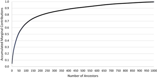
Accumulated marginal contributions by number of ancestors.
Pairwise animal connectedness based on pedigree is shown in Figure 2a–c. The PC1, PC2, and PC3 explained 8.0%, 4.6%, and 4.4% of the variation in the population, respectively. Each PC pairing shows separation among some flocks with clustering among the remaining flocks. Flocks that are more distinct from the others are 2, 5, and 7.
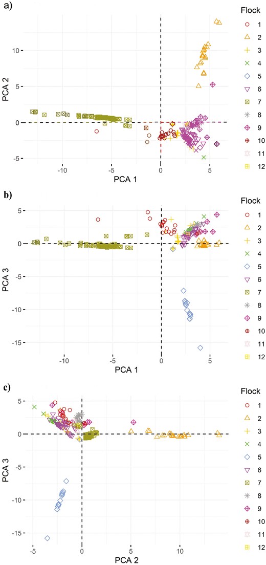
Plot of PC1 and PC2 (a), PC1 and PC3 (b), and PC2 and PC3 (c) for pairwise correlation coefficients among animals, grouped by flock.
Molecular Analyses
For genotyped US Suffolk sheep, the molecular measures of genetic diversity were 0.317 for HE, 0.306 for HO, and 0.035 for FIS. Minor allele frequency distributions are presented in Table 3, showing no variation (fixed) for 6.4% of SNP and low variation (rare) for 4.0% of SNP. High variation was observed for 34.5% of SNP.
Minor allele frequency (MAF) distribution of US Suffolk sheep (n = 564 341 SNP)
| MAF category | % of SNP |
|---|---|
| Fixed (0) | 6.4 |
| Rare (<0.01) | 4.0 |
| Moderate (0.01–0.3) | 55.1 |
| High (0.3–0.5) | 34.5 |
| MAF category | % of SNP |
|---|---|
| Fixed (0) | 6.4 |
| Rare (<0.01) | 4.0 |
| Moderate (0.01–0.3) | 55.1 |
| High (0.3–0.5) | 34.5 |
Historical Ne (Figure 3) shows a linear decrease in Ne from 100 generations ago to the most recent generation computed (13 generations ago). In that time, Ne decreased from more than 600 to 251 in the US Suffolk population. The current Ne in 2019 was 79.5.
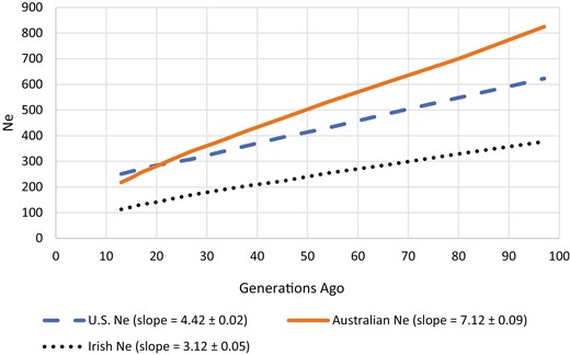
Historical effective population size (Ne) ranging from 13 to 100 generations ago for US, Australian, and Irish Suffolk sheep.
Model-based population structure analysis identified 7 subpopulations (Figure 4). Pairwise FST between flocks showed flocks 2, 5 and 7 had the most differentiation from the others (Table 4). Such is also reflected in the model-based population structure as relatively distinct subpopulations (yellow, brown, and blue, respectively) in Figure 4 and in flock connectedness in Figure 2.
FST (upper diagonal) and 95% confidence intervals (lower diagonal) by flock
| 1 | 2 | 3 | 4 | 5 | 6 | 7 | |
|---|---|---|---|---|---|---|---|
| 1 | 0.105 | 0.040 | 0.058 | 0.098 | 0.049 | 0.060 | |
| 2 | 0.1037, 0.1066 | 0.104 | 0.106 | 0.097 | 0.063 | 0.101 | |
| 3 | 0.0396, 0.0413 | 0.1028, 0.1060 | 0.039 | 0.094 | 0.034 | 0.049 | |
| 4 | 0.0565, 0.0587 | 0.1044, 0.1080 | 0.0384, 0.0401 | 0.090 | 0.043 | 0.068 | |
| 5 | 0.0969, 0.0997 | 0.0959, 0.0986 | 0.0924, 0.0952 | 0.0888, 0.0913 | 0.070 | 0.096 | |
| 6 | 0.0478, 0.0496 | 0.0624, 0.0644 | 0.0332, 0.0346 | 0.0419, 0.0432 | 0.0687, 0.0704 | 0.054 | |
| 7 | 0.0584, 0.0604 | 0.0991, 0.1020 | 0.0483, 0.0498 | 0.0668, 0.0685 | 0.0950, 0.0978 | 0.0537, 0.0553 |
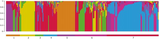
Model-based population structure for K = 7, sorted by flock. Only flocks with 10 or more genotyped animals were included in the analysis.
International Comparison
Measures of molecular genetic diversity are presented in Table 5 for the United States, Australian, and Irish Suffolk sheep. The Australian Suffolk population had the highest Ne and lowest FIS, followed by the US population, and then the Irish population. Historical Ne (Figure 3) shows a steeper slope for the Australian Suffolk followed by the United States and Ireland. Of note, the US population has a higher Ne than the Australian population from generation 13 to 20. Computed Ne using three methods is shown in Table 6, where Australian Ne is consistently the highest and Irish Ne is the lowest. FST between countries was 0.062, 0.064, and 0.076, with a corresponding migration rate of 0.05, 0.05, and 0.04 between the United States and Australia, the United States and Ireland, and Australia and Ireland, respectively.
HE, HO, and FIS for US, Australian, and Irish Suffolk sheep (n = 25 496 SNP)
| Country | n | HE | HO | FIS |
|---|---|---|---|---|
| United States | 303 | 0.363 | 0.333 | 0.081 |
| Australia | 109 | 0.363 | 0.373 | −0.028 |
| Ireland | 55 | 0.363 | 0.314 | 0.134 |
| Overall | 467 | 0.363 | 0.340 | 0.062 |
| Country | n | HE | HO | FIS |
|---|---|---|---|---|
| United States | 303 | 0.363 | 0.333 | 0.081 |
| Australia | 109 | 0.363 | 0.373 | −0.028 |
| Ireland | 55 | 0.363 | 0.314 | 0.134 |
| Overall | 467 | 0.363 | 0.340 | 0.062 |
Molecular-based estimates of Ne for US, Australian, and Irish Suffolk sheep (n = 41 471 SNP)
| Country | LD based Ne | Heterozygote excess Ne | Molecular coancestry Ne | Kijas et al. 2012 LD based Ne |
|---|---|---|---|---|
| United States | 76.3 | N/A | N/A | N/A |
| Australia | 104.1 | 400.8 | 5.0 | 569 |
| Ireland | 22.7 | N/A | 1.1 | 300 |
| Country | LD based Ne | Heterozygote excess Ne | Molecular coancestry Ne | Kijas et al. 2012 LD based Ne |
|---|---|---|---|---|
| United States | 76.3 | N/A | N/A | N/A |
| Australia | 104.1 | 400.8 | 5.0 | 569 |
| Ireland | 22.7 | N/A | 1.1 | 300 |
Based on PCA of the merged SNP from the three countries, the first three PC explained 28.4%, 15.6%, and 14.4% of the variation in the population, respectively. A comparison of PC1 and PC2 (Figure 5a) shows a clear separation of the US and Australian populations. PC1 and PC3 (Figure 5b) shows differentiation among all three countries, while PC2 and PC3 (Figure 5c) separates the Irish Suffolk from the US and Australian populations. Similarly, model-based population structure, illustrated for K = 2 to K = 4 (Figure 6), also shows a clear separation between the United States, Australian, and Irish Suffolk populations.
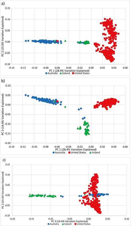
Plot of PC1 and PC2 (a), PC1 and PC3 (b), and PC2 and PC3 (c) for US, Australian, and Irish Suffolk sheep.
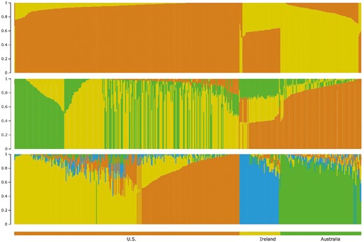
Model-based population structure for K = 2 to K = 4 for US, Australian, and Irish Suffolk sheep.
Flock Connectedness
Pedigree-based flock connectedness among 4 clusters and 12 individual flocks is presented in Figure 7. Six flocks with low connectedness are excluded from the diagram including flocks 5 and 7 but not flock 2. When all 18 flocks are considered, every flock has at least one relationship to one other cluster and 4 flocks are connected to all clusters. Of the moderate to high relationships shown in Figure 7, flock 2 is only connected to flock 19 (within cluster), and flock 13 is only connected to flock 15 (between clusters).
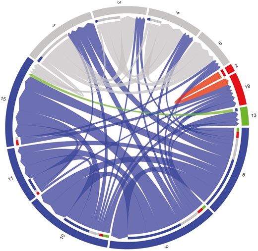
Connectedness among flocks with NSIP participation showing 4 clusters (color) and 12 individual flocks (number). Six flocks with low connectedness are excluded from the diagram.
Accuracies of Genomic-Enhanced Estimated Breeding Values
Using the computed molecular-based current Ne of 79.5 and a genome length of 34.3 Morgans, predicted accuracies for GS are presented in Table 7. Accuracies range from a low of 0.092 with a reference population size of 250 and a heritability of 0.1 to a high of 0.792 with a reference population size of 10 000 and a heritability of 0.4. These are baseline accuracies for animals with no direct relatives in the reference population and no phenotype for the trait of interest.
Genomic-enhanced estimated breeding value accuracies with varying reference population size and heritabilities
| Reference population size | |||||||
|---|---|---|---|---|---|---|---|
| 250 | 500 | 1000 | 3000 | 5000 | 10 000 | ||
| Heritability | 0.1 | 0.092 | 0.130 | 0.182 | 0.303 | 0.378 | 0.495 |
| 0.2 | 0.138 | 0.192 | 0.266 | 0.427 | 0.516 | 0.640 | |
| 0.3 | 0.179 | 0.248 | 0.339 | 0.521 | 0.613 | 0.729 | |
| 0.4 | 0.221 | 0.303 | 0.407 | 0.601 | 0.689 | 0.792 | |
Discussion
In this study, we evaluated genetic diversity and population structure of a subset of Suffolk sheep. We demonstrated that genetic diversity has declined over time and there was presence of population substructure. However, the combination of substantial genetic distances between flocks and the low marginal contribution of individual animals to the population provides significant opportunity and flexibility to minimize inbreeding through new allelic combinations. Our findings provide an understanding of the past and present genetic profile of the breed and guidance for GS moving forward.
The 1704 animals recorded in the NSIP in 2019 represent one-third of all Suffolk registrations. Unlike the US beef and dairy breeds that participate in genetic evaluation through their breed associations, individual breeders elect whether to participate in NSIP. This results in breeders entering and exiting NSIP over time, leading to incomplete pedigree data and lower genetic connectedness among flocks. Kuehn et al. (2009) identified this issue more than a decade ago and found the problem to be greater in the Suffolk than Targhee breed. Those authors also identified divergent selection within Suffolk for differing breeding objectives leading to less sharing of germplasm even amongst flocks in close physical proximity.
The 2019 average flock size was 57.3 animals; flocks of this size are typically dominated by genetic drift which impedes genetic improvement (Nicholas 1980; Blackburn et al. 2018). Although genetic trends in NSIP show gains are being achieved (Sheep Industry News 2017), greater responses would be expected without the counteracting effects of genetic drift. The rate of change of inbreeding appeared constant across years; as expected, accumulation of inbreeding is decreasing Ne over time. The mean generation interval (2.9 years) was lower than reported for Canadian Suffolk (3.3 years) (Stachowicz et al. 2018).
The much smaller numbers for (107) and (50) relative to (255) suggest significant bottlenecks and, more likely, genetic drift acting on this population. In comparison, in Canadian Suffolk , , and were 139, 79, and 168, respectively (Stachowicz et al. 2018). Accumulated marginal contributions show a lack of highly influential individuals in the population; this is partially explained by the absence of the wide use of advanced reproductive technologies such as artificial insemination (AI) and embryo transfer, plus differing selection objectives (Kuehn et al. 2009). While advanced reproductive technologies are common in other livestock species, they are infrequently used in sheep. This is due to the high cost of laparoscopic AI, which is a procedure conducted by a veterinarian, and the inconsistent conception rates achieved with noninvasive cervical AI (Wildeus et al. 2018; Alvarez et al. 2019; Purdy et al. 2020). This contributes to reduced gene flow and less connectedness between flocks and countries because rams must be physically moved rather than shared among flocks through AI.
Marginal contributions by the top 10 animals ranged from 15 to 355 offspring in contrast with thousands of offspring produced by major beef and dairy sires (American Angus Association 2021; Funk 2006; Fennewald et al. 2017). The top 10 marginal contributors explained 22.8% of the current gene pool; this is low compared to a range of 46.7 to 84.0% of the current gene pool for the top 10 marginal contributors for 5 Canadian dairy cattle breeds (Melka et al. 2013). For 5 Canadian sheep breeds, 10 to 52 ancestors explained 50%of the current gene pool, including 52 ancestors for Canadian Suffolk (Stachowicz et al. 2018); 46 ancestors explained the same amount for the NSIP Suffolk population, a subpopulation of US Suffolk.
Among SNP, 93.6% were polymorphic, which is higher than that reported by Kijas et al. (2014) of 90.9% for Suffolk sheep using the OvineHD BeadChip. The level of genetic diversity present within a population can be measured by the number of polymorphic loci and their allele frequency distributions (Brito et al. 2015). Only 4% of SNPs were classified as rare (<0.01) while almost 90% were classified in the polymorphic categories of moderate or high, suggesting significant variation exists in the breed.
Even with significant allelic variation, the current Ne (79.5) in US Suffolk is below the minimum of 100 recommended by Meuwissen (2009), although above the minimum of 50 recommended by the FAO (1998). It also exceeds the Holstein estimate of 58, a numerically larger breed (Makanjuola et al. 2020). The effective population size has declined substantially across the past 100 generations (about the time the breed was first established in 1791), but this pattern and magnitude of decay are typical for livestock populations (Faria et al. 2019; McHugo et al. 2019; Makanjuola et al. 2020). At present, Ne and FIS suggest loss of genetic diversity in Suffolk is smaller than breeds with much larger populations (Holstein, Jersey, Duroc, Yorkshire). Nonetheless, steps to conserve the remaining genetic variation deserve attention (Taberlet et al. 2011). Particularly once GS is implemented, the rate of inbreeding will likely increase. Breeders need to be made fully aware of such a prospect and plan accordingly to ensure the long-term sustainability of the breed.
Based on the PCA, subpopulations exist within the breed that are not based on geographical distance (results not shown); similar results were reported for subpopulations within Yorkshire and Meishan pig breeds (Faria et al. 2019). Model-based population structure, pedigree-based animal connectedness, and FST show separation among flocks, which supports observations by Kuehn et al. (2009) about differential selection within US Suffolk. Breeder interest in different selection criteria, combined with a low marginal contribution of individual animals, provides an opportunity for the breeders to maintain outcross subpopulations or, alternatively, to cross the distant populations to generate new allelic combinations.
When the US population was compared to Irish and Australian populations, genetic diversity as estimated by HE was equivalent across samples. Nevertheless, FIS measures revealed a greater degree of inbreeding in the US and Irish samples compared to that in Australia. The Australian population, however, had a greater negative slope for Ne, suggesting genetic diversity is being lost at a higher rate. The elevated FIS in the United States could be the result of a Wahlund effect (Sinnock 1975), since there was evidence of heterozygote deficits in subpopulations among US Suffolk flocks.
Estimates of Ne are important to assess the potential loss of genetic diversity in a population and in computing accuracies for genomic selection, but consistent results are difficult to achieve. Goyache et al. (2011) cautioned about the use of molecular-based Ne estimates in livestock conservation programs. England et al. (2006) found the standard LD method to be biased when sample size was less than the true Ne. The NeEstimator software (Do et al. 2014) used in the current analyses makes a correction for this bias. The LD method used by Kijas et al. (2012) for the Australian and Irish Suffolk estimated 569 and 300, respectively. For the same populations, we estimated 104 and 23, respectively. The correction for bias in the NeEstimator software may provide some insight into these differences considering the population sizes were only 109 and 55 for the Australian and Irish Suffolk, respectively. Additionally, Kijas et al. (2012) assumed the distance between SNP was 100Mb = 1 Morgan, where 100Mb = 1.5 Morgans has also been determined to be appropriate (Petit et al. 2017). Ne studies may be most beneficial when comparing populations using the same sampling strategies and methodologies, and not across studies. If loss of genetic diversity is of interest in a single population over time, care must be taken to ensure the same sampling and methodologies are used. Trends and rankings may be more informative than the individual estimates.
Across the three countries, genetically separate Suffolk populations were identified with a few admixed animals (Figure 5a–c). Some migration was evident between countries with a migration rate ranging from 0.04 to 0.05 (3–4 animals per generation). The Irish population appears intermediate between the United States and Australian populations in both the parametric (Figure 6) and nonparametric (Figure 5a–c) analyses. The Irish population only becomes its own subpopulation when K = 4 in the parametric analysis (Figure 6). While the Suffolk breed serves as a terminal sire breed in all three countries, selection objectives and genetic isolation by distance would be expected to result in the differentiation observed.
As the US livestock industry entered the postgenomic era, GS has become routine for beef, dairy, swine, and poultry. It is now time for the sheep industry to capitalize on the advances that have been made while also avoiding the drawbacks other species have experienced. One example that the sheep industry can learn from is that observed with the dairy cattle industry. High LD has led to successful GS and an increase in selection intensity. However, this has been followed by a loss of genetic diversity because of relatively high rate of inbreeding and associated reduction in Ne (Makanjuola et al. 2020). In sheep this situation may be offset by lower LD, which also makes GS more challenging (Rupp et al. 2016).
An in-depth understanding of the population structure and genetic diversity provides a basis for developing a GS strategy. Based on flock connectedness, sires from each cluster and from the relatively disconnected clusters should be sampled for HD genotyping to establish a reference population. Sampling connected and relatively disconnected flocks, in combination with optimal contribution selection (Woolliams et al. 2015; Eynard et al. 2018), will promote maintenance of genetic diversity.
Globally, there is a need to increase the efficiency of animal protein production to meet the world’s needs, with estimates as high as a 10-fold increase in the rate of genetic improvement being required (Rexroad et al. 2019). GS has the potential for a doubling of genetic gain (van der Werf et al. 2014), making its implementation of critical importance. In the United States, GS has added a value of $50 per dairy cow per year (Rexroad et al. 2019), suggesting the increase in accuracy from GS justifies the expense; however, it is doubtful that such a high value can be achieved in sheep. A large reference population size is needed to take advantage of the increased accuracy from GS. For example, given the heritability of 0.15 used by NSIP for weaning weight in Suffolk, reference population sizes of 250, 3000, and 10 000 would result in accuracies of 0.116, 0.371, and 0.578, respectively, for GEBV. Given these values, a minimum of 3000 animals should be genotyped to meet breeder expectations of increased accuracy.
Conclusion
Genetic diversity has decreased in the Suffolk population, as shown by the values of fa and Ng relative to fe, and a decreasing Ne, trends also seen in other breeds under selection. However, sufficient variation exists as measured by HE, few fixed SNP, and significant divergence among flocks. Pedigree- and genomic-based discrimination of relationships shows a consistent separation of the same flocks. Connectedness among flocks provides the opportunity to develop a reference population for GS while disconnectedness among other flocks provides the opportunity to maintain genetic diversity within the breed.
The population structure of the US Suffolk breed that is actively participating in genetic evaluation is the basis for developing a reference population for GS. Establishment of GS will position the US Suffolk breed for advances in genetic gain for all measured traits and an opportunity to improve novel yet economically relevant traits currently absent from breeding objectives.
Funding
The authors would like to acknowledge the sources of funding for the genotyping portion of the project, including FTA cards collected from NSIP enrolled flocks funded by an American Sheep Industry Association Let’s Grow Grant, genotyping of 64 Suffolk sheep by Neogen Corporation in-kind support of research at the University of Nebraska-Lincoln, genotyping of 180 Suffolk sheep provided by the Agricultural Research Service Innovation Fund, and genotypes from 60 Suffolk rams provided by United States Department of Agriculture, Agricultural Research Service, National Animal Germplasm Program.
Acknowledgments
We thank the National Sheep Improvement Program (NSIP) Executive and Board for access to pedigree and performance data, and the 10 NSIP Suffolk breeders who provided DNA samples from their flocks. We also thank Dr. James Kijas for providing the Australian and Irish Suffolk SNP data. USDA is an equal opportunity employer and provider. We thank the Associate Editor and our reviewer for suggestions for improving this manuscript.
Data Availability
We have deposited the primary data underlying these analyses in the Dryad Digital Repository (https://doi.org/10.5061/dryad.ttdz08m1t).
References
