


Abstract
Few doubt that effective population size (Ne) is one of the most important parameters in evolutionary biology, but how many can say they really understand the concept? Ne is the evolutionary analog of the number of individuals (or adults) in the population, N. Whereas ecological consequences of population size depend on N, evolutionary consequences (rates of loss of genetic diversity and increase in inbreeding; relative effectiveness of selection) depend on Ne. Formal definitions typically relate effective size to a key population genetic parameter, such as loss of heterozygosity or variance in allele frequency. However, for practical application to real populations, it is more useful to define Ne in terms of 3 demographic parameters: number of potential parents (adult N), and mean and variance in offspring number. Defined this way, Ne determines the rate of random genetic drift across the entire genome in the offspring generation. Other evolutionary forces (mutation, migration, selection)—together with factors such as variation in recombination rate—can also affect genetic variation, and this leads to heterogeneity across the genome in observed rates of genetic change. For some, it has been convenient to interpret this heterogeneity in terms of heterogeneity in Ne, but unfortunately, this has muddled the concepts of genetic drift and effective population size. A commonly repeated misconception is that Ne is the number of parents that actually contribute genes to the next generation (NP). In reality, NP can be smaller or larger than Ne, and the NP/Ne ratio depends on the sex ratio, the mean and variance in offspring number, and whether inbreeding or variance Ne is of interest.
Nature uses only the longest threads to weave her patterns, so that each small piece of her fabric reveals the organization of the entire tapestry (Feynman 1964).
Effective population size is the primary thread in the tapestry of population genetics (Allendorf FW, Personal communication to the author).
Recently, a colleague posed to me a rather philosophical question about effective population size:
‘Ne determines rates of genetic drift and loss of genetic variability’ (Waples 2016a, p. 4689). To me, this statement is backwards. That is, the rate of genetic drift determines Ne, not vice versa. Ne is not a physical entity (as is, say, allele frequencies). Rather, Ne is a conceptual entity that we use to measure genetic drift.
After some other colleagues were drawn into the ensuing email exchange, one suggested I write up my ideas, and this Perspective is the result. The initial question is another way of asking, “What the heck is Ne, anyway?”—hence the title.
I have been asked questions like this many times, and I expect others have as well. Effective population size (Ne) is an elegantly simple concept, but also a slippery one that is hard to pin down. Just when you think you understand it, a new wrinkle appears that gives you pause. We all have heard textbook definitions that go something like this: “Ne is the size of an ideal population that would experience the same rate of genetic drift as the population in question.” And an “ideal” population is one with discrete generations that mates randomly, experiences no evolutionary forces besides genetic drift, and within which all individuals have an equal probability of producing offspring. Although this definition of Ne is technically correct, I doubt it has actually led to much enlightenment in most readers; one can repeat definitions like these without understanding what they actually mean. In school I experienced the same problem trying to understand the definition of a limit: “the limit of f(x) as x→c = L means that for every ϵ > 0, there exists a δ > 0, such that . . .” yada yada yada. I memorized this verbatim and could regurgitate the definition on a test, but without really grasping the underlying concept. (See https://www.youtube.com/watch?v=zxFCQplZgKI&t=151s for Tom Lehrer’s take on this “epsilon-delta” problem.) It was not until much later (perhaps with a little pharmaceutical help—I can’t remember now) that I could really say that I grokked what a limit is.
Grokking Ne
Truly understanding Ne deeply and intuitively (i.e., grokking Ne) is equally challenging. For me the simplest way to think about the problem is that Ne is just a number, akin to but generally different from, the number of individuals in the population, N. Ecological processes like competition, predation, density dependence, population growth rates, and disease transmission all depend on census size. For example, if one wants to model epidemiology in a global pandemic, one uses equations that depend, among other things, on the parameter N. In contrast, rates of evolutionary processes depend on Ne.
Four evolutionary forces shape genetic diversity within and among populations: mutation, migration, selection, and genetic drift. Of the 4, genetic drift is distinctive for 2 reasons. First, drift is inherently a stochastic process whose outcomes can only be predicted in a statistical sense. In contrast, the other evolutionary forces all shape genetic change in a specific direction. Second, whereas mutation, migration, and selection might or might not be relevant for any given time period or site in the genome, all real populations are finite, so genetic drift affects the entire genome in every generation. Ne determines the expected rate of genetic drift, and that is why essentially all equations in evolutionary biology include a term for Ne.
A complication is that multiple “flavors” of Ne have been defined in the literature—not as many as species concepts, but enough to cause some confusion. The 2 most widely used are the inbreeding and variance effective sizes, first distinguished by Crow (1954). The 2 effective sizes are the same in isolated populations of constant size but differ otherwise, with inbreeding Ne reflecting the number in the parental generation and variance Ne the number in the offspring generation. Both inbreeding and variance effective size most commonly refer to evolutionary processes in one or a few recent generations (hence contemporary Ne), and in this respect, they differ markedly from the concept of a long-term effective size, which focuses on the composite parameter θ = 4Neμ, where μ is mutation rate (Watterson 1975). Under the infinite-allele mutation model, at mutation-drift equilibrium the expected level of heterozygosity is given by (Hedrick 2000):
The amount of genetic variation in a population thus reflects a balance between mutation (which increases genetic diversity) and genetic drift (which reduces it). Recent authors (e.g., Sjödin et al. 2005; Wakeley and Sargsyan 2009) have defined the effective size term in θ to be a coalescent Ne that exists when, in the limit as N→∞, the evolutionary processes responsible for genetic variation converge on the Kingman coalescent. Equation 1 depends on the assumptions that mutations are neutral and the population is completely isolated for long enough to reach mutation-drift equilibrium. With even small amounts of migration, the amount of genetic diversity within a local population will reflect the metapopulation or even species-wide effective size rather than the local Ne.
Between these extremes, improvements in genomics technology and analytical capabilities have opened up opportunities to attempt to reconstruct historical demography across a wide range of temporal scales. Interested readers can consult useful reviews of “skyline plot” methods to estimate historical Ne based on coalescent theory (Ho and Shapiro 2011) and the entire temporal continuum of Ne estimation methods, including future prospects (Nadachowska-Brzyska et al. 2022).
Definitions of Ne
If Ne is a number, how does one determine what that number is? For this we need a formal definition. Quite a bit has been written about how to estimate effective size based on samples (e.g., Luikart et al. 2010; Wang et al. 2016; Nadachowska-Brzyska et al. 2022), but here I want to focus on the parametric value that can be considered to be the “true” Ne for a population for a specific time period. In the theoretical population genetics literature, Ne is generally defined in relation to a key evolutionary metric. For inbreeding effective size, the key metric is the probability (P) that a pair of homologous genes in an individual came from the same parent in the previous generation. In the original Wright–Fisher ideal population (a monoecious diploid with random self-fertilization), this probability is simply the inverse of the number of ideal parents, N (Kimura and Crow 1963):
The great value of the effective size concept is that it allows one to replace “N” in Equation 2 (and related equations) with a new term that captures more of the realistic features of actual populations. We still assume random mating and limit consideration to just one of the evolutionary forces (genetic drift), but we are relaxing a key restrictive assumption of an ideal population: that each adult is equally likely to be the parent of every offspring. With separate sexes, this also allows for the possibility of a skewed sex ratio. In a large meta-analysis, Frankham (1995) found that, for a single generation of reproduction, in combination these 2 factors (uneven sex ratio and greater-than-random variation in offspring number among individuals of the same sex) reduced the mean Ne to 35% of the number of adults.
If one substitutes Ne for N and rearranges Equation 2, the result is a new equation that defines Ne in terms of the probability that 2 homologous genes in a randomly chosen offspring came from the same parent (Kimura and Crow 1963; Crow and Kimura 1970):
For variance effective size, the analogous approach is to describe the parametric relationship between the number of ideal individuals (N) and the variance in allele frequency (Vp) across many replicate daughter populations, or many replicate gene loci:
with p0 being the initial allele frequency in the parental generation. Rearrangement and substituting for N then produces the variance Ne analog of Equation 3 (Crow and Kimura 1970):
Equation 4 applies to a single generation of drift; it can be extended to give the expected variance in allele frequency ( after t generations of drift, assuming a constant effective size (Hedrick 2000):
Moving from numbers of ideal individuals (Equations 2 and 4) to effective population sizes (Equations 3 and 5) is a neat trick that has proved to be enormously useful for both theoretical and empirical population genetics. However, this approach to defining Ne has one serious drawback: it is not operational in any practical sense. In theory, one could calculate a true variance Ne by quantifying the right side of Equation 5 or 6, using data for all genes. With modern genomics methods, it certainly is possible to compute allele frequencies across the whole genome at any time point for which appropriate samples can be collected, and from these data it is straightforward to calculate variances in allele frequency for each site (e.g., see Nei and Tajima 1981). But the relationships in Equations 5 and 6 hold only for sites that experience no evolutionary forces besides genetic drift. How can one identify those sites that, over the generation(s) in question, were completely unaffected by mutation, migration, and selection? For all practical purposes, that is impossible to achieve.
Fortunately, there is a simple solution to this problem: Ne can also be defined based on 3 demographic parameters of the population: the number of potential parents (N), and the mean and variance in the number of offspring per parent (k). For a monoecious diploid with random self-fertilization, the discrete-generation inbreeding and variance effective sizes are defined as:
and slight variations are available for other mating systems (Crow and Denniston 1988; Caballero 1994). The 2 effective sizes are the same when population size is constant (), but variance Ne is larger in growing populations and inbreeding Ne is larger when populations decline in size. Inspection of Equations 7 and 8 makes clear the importance of the ratio of the variance to mean offspring number (ϕ=/), which Crow and Morton (1955) called the “Index of Variability.” In a Wright–Fisher “ideal” population, the variance in offspring number is binomial (effectively Poisson unless N is very small), with the result that ϕ ≈ 1 and Ne ≈ N, but this scenario applies to few real populations.
Equations 7 and 8 have the following meaning: if mean and variance in offspring number are recorded for all potential parents and used to compute Ne, and if that result is used for N in formulas for genetic drift like Equations 2 or 4, those equations will accurately predict the rates of increase in inbreeding and increase in allele frequency variance. To take a concrete example, Buri (1956) conducted a famous experiment in which he tracked change over time in the frequency of 2 apparently neutral eye-color genes in replicate laboratory populations of Drosophila melanogaster. He controlled population size at 8 males and 8 females each generation but did not control distribution of offspring number. Across 20 generations he found good agreement between the empirical and theoretical predictions based on Equation 6 assuming a constant Ne = 9, suggesting that effective size was a bit over half of the number of adults.
Buri had access to only a single gene locus and so monitored the variance across replicate daughter populations (easy to do in a computer, and possible in a laboratory with Drosophila), but Equation 6 also can be applied to replicate neutral genes. The standardized variance, is independent of initial allele frequency, which facilitates combining results across replicates with different initial conditions (Krimbas and Tsakas 1971). To illustrate, assume that 100 potential parents produce 100 offspring (so μk = 2, with each parent on average providing half the genes to 2 offspring) but the variance in offspring number is overdispersed, such that = 5, or 2.5 times as large as the Poisson variance. Because population size is stable, variance and inbreeding effective sizes are the same, and Ne = 56.9 using either Equation 7 or 8 (so Ne/N = 0.57, very similar to the value Ne/N = 9/16 = 0.56 estimated in Buri’s experiment). I simulated 20 generations of genetic drift in many replicates of a closed population having these demographic parameters, and frequencies were tracked for large numbers of neutral, diallelic loci, all starting with initial frequency p0 = 0.5. The distribution of offspring number was controlled to ensure that that ≈ 5 and Ne ≈ 57 every generation (see Supplementary Material). Results (Figure 1 and Supplementary Figure S1) show that (1) on average, the replicate populations follow the expected temporal trajectory of increasing allele frequency variance, per Equation 6; and (2) random stochasticity inherent to genetic drift can be reduced by averaging across many genes and many replicate populations.

Rate of increase in variance of allele frequency over time in simulated populations with N = 100 potential parents, = 5, and Ne = 56.9. Vp was averaged over 50 (top) or 5000 (bottom) neutral, diallelic loci, all starting with initial frequency p0 = 0.5. Each colored line shows empirical data for one replicate population followed for 20 generations. Filled circles are from Equation 6 using Ne = 56.9.
Natural selection has an interesting and complex interaction with Ne. Because selection involves differential survival and/or reproduction of individuals with different phenotypes, it generally increases and reduces effective population size. The resulting Ne (from Equation 7 or 8) then governs the rate of genetic drift across the genome, but a new episode of selection can then modulate the drift signal at specific genomic regions that are directly associated with selected phenotypes, or linked to sites that are. Somewhat ironically, strong selection that substantially increases and hence substantially reduces Ne will also make selection in general less effective at other sites in the genome. In large populations, even weak selection can predictably shape genetic variation, due to the law of large numbers: with sufficient replication of a chance event, the mean outcome will converge on the theoretically expected value. A direct analogy to a selection coefficient is the house margin in a gambling establishment: in a large casino the house margin can be small because the high volume guarantees that, inexorably, the house will eventually come out ahead. In contrast, a convenience store with a single gambling machine needs a larger margin to minimize the chance of catastrophic loss due to one or a few lucky customers.
Robertson (1961) described a scenario under which Equations 7 or 8 might overestimate Ne across the genome: if fitness itself is heritable (such that parents from large families also produce large families), the cumulative effects of selection across multiple generations can reduce effective population size, leading to higher rates of genetic drift than predicted by these equations. This idea has been further developed and generalized by Nei and Murata (1966) and by Santiago and Caballero (1995), who defined an asymptotic effective size that reflects cumulative effects of constant selection over long time periods. Although Robertson’s initial formulation of this idea was for an artificial selection program in animal husbandry, the same principle potentially applies to natural selection in real populations, which can exhibit heritability of fitness (Hill and Zhang 2009). If fitness is heritable, asymptotic Ne is a function of N, the strength of selection, heritability of fitness, and mating structure (Nei and Murata 1966; Santiago and Caballero 1995). This asymptotic effective size will be smaller than values obtained from Equations 7 or 8 (which only account for a single generation of demographic variance) and it will govern the rate of genetic drift across the genome, not just at sites directly associated with fitness.
Something That Is NOT Ne
One often encounters statements like the following in journal articles or even textbooks: “Effective population size is the number of individuals that contribute offspring to the next generation.” Although it is possible to find scenarios where this statement holds, it is not true in any general sense. For example, if variation in offspring number is random and mean offspring number is μk = 2 (indicating a stable population), then (based on the binomial distribution) we know that on average almost one in 7 potential parents will leave no offspring, just by chance. In that scenario, the number of parents contributing at least one offspring (NP) is about 13%–14% less than Ne (Figure 2, black bars). In the extreme case where all individuals produce the same number of offspring (= 0), Ne ≈ 2N so NP is about half of Ne. Conversely, if reproductive success is skewed, NP can be higher than Ne (about 14% higher in the example shown in Figure 2, gray bars, where is 5 times the mean and Ne/N = 0.33). With separate sexes, the NP/Ne ratio is sensitive to the sex ratio and can be 2 or higher when the sex ratio is highly skewed (e.g., 1:10; Table 1).
Variation in the NP/Ne ratio as a function of the male:female sex ratio in populations that are otherwise ideal. Values in the table show total numbers of males and females, M:F sex ratio, expected numbers of each sex that produce at least one offspring (Male NP, Female NP), effective population size (Ne), and the overall NP/Ne ratio across both sexes. Expected NP was calculated using the dbinom function in R to predict the number of null parents, and Ne was calculated using Wright’s formula Ne = 4*Males*Females/(Males + Females). As the sex ratio becomes more female biased, female Np increases almost linearly with the number of females, whereas overall Ne is increasingly constrained by the asymptotic value of Ne = 4*Males. As a consequence, the ratio Np/Ne more than doubles when sex ratio changes from 1:1 to 1:10
| Males | Females | Sex ratio | Male NP | Female NP | N P | N e | N P/Ne |
|---|---|---|---|---|---|---|---|
| 50 | 50 | 1:1 | 43.4 | 43.4 | 86.7 | 100.0 | 0.87 |
| 50 | 100 | 1:2 | 47.6 | 77.9 | 125.4 | 133.3 | 0.94 |
| 50 | 150 | 1:3 | 49.1 | 110.6 | 159.8 | 150.0 | 1.07 |
| 50 | 200 | 1:4 | 49.7 | 142.9 | 192.6 | 160.0 | 1.20 |
| 50 | 250 | 1:5 | 49.9 | 174.9 | 224.8 | 166.7 | 1.35 |
| 50 | 300 | 1:6 | 50.0 | 206.8 | 256.7 | 171.4 | 1.50 |
| 50 | 350 | 1:7 | 50.0 | 238.6 | 288.5 | 175.0 | 1.65 |
| 50 | 400 | 1:8 | 50.0 | 270.3 | 320.3 | 177.8 | 1.80 |
| 50 | 450 | 1:9 | 50.0 | 302.0 | 352.0 | 180.0 | 1.96 |
| 50 | 500 | 1:10 | 50.0 | 333.7 | 383.7 | 181.8 | 2.11 |
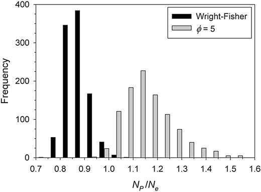
The ratio of the number of parents producing at least one offspring (NP) to Ne in simulated populations. Two scenarios were simulated, both with N = 100 potential parents producing an average of 2 offspring each: 1) Wright–Fisher reproduction, in which (on average) Ne = N and 2) more realistic demography, in which the ratio of variance to mean number of offspring was , leading to expected Ne/N = 0.33. In both scenarios, results shown include data from 1000 replicate generations of reproduction. Median values of the ratio NP/Ne were 0.86 for Scenario 1 and 1.14 for Scenario 2. The simulations used methods described in more detail in Supplementary Material.
Furthermore, the fraction of potential parents that produce at least one offspring (NP/N) increases with mean offspring number and asymptotically approaches 1 as μk becomes large (null parents become increasingly unlikely when each potential parent has a large number of opportunities to reproduce). Because inbreeding Ne is invariant with μk, while variance Ne is proportional to μk (Figure 3), the general relationship between Ne and NP is complex (Figure 4) and depends on mean offspring number and degree of reproductive skew, as well as which effective size is used.
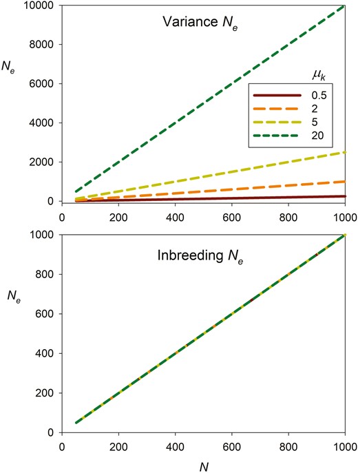
Contrasting effects of mean number of offspring per parent (μk) on variance Ne (top) and inbreeding Ne (bottom). The X axis plots the number of ideal individuals in the population (N). Results are based on Equations 7 and 8 assuming random reproductive success, so , in which case inbreeding Ne = N regardless of mean offspring number, whereas variance Ne is proportional to μk.
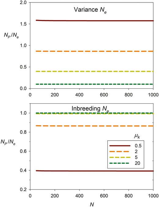
Contrasting effects of mean number of offspring per parent (μk) on the NP/Ne ratio for variance Ne (top) and inbreeding Ne (bottom). NP is the number of parents producing at least one offspring, and the X axis plots the number of ideal individuals in the population (N), who are assumed to have random reproductive success. Ne values are the same as those in Figure 3, and NP was calculated using the dbinom function in R.
Finally, all of these analyses assumed discrete generations, whereas most species in nature are age structured. I am not aware of any systematic evaluations of the NP/Ne ratio in species with overlapping generations, but it is reasonable to expect that it will be influenced by a variety of factors, including the mating system (Nunney 1993), longevity (Waples 2016b), the adult sex ratio (Nunney and Elam 1994), patterns of age-specific survival and fecundity (Felsenstein 1971; Nunney 1996), the index of variability for individuals of the same age and sex (Waples et al. 2011), intermittent breeding (Shaw and Levin 2011), and persistent individual differences (Lee et al. 2011).
Does Ne Vary Across the Genome?
A logical corollary of the demographic definition of Ne is that the same effective size applies to the entire autosomal portion of a genome, with simple adjustments for sex chromosomes or organelles. This does NOT imply that rates of genetic change at all sites will be determined solely by Equations like 2, 4, and 6; it only implies that the component of genetic change attributable to genetic drift will be governed by those equations. The net changes at any given site in any given generation will always be influenced by genetic drift but might also be affected by the other evolutionary forces (mutation, migration, selection), and perhaps also by other factors, such as nonrandom mating and variation in recombination rate. This makes the analysis of genetic change experienced by real populations much more complicated. Fortunately, the joint effects of genetic drift and the other evolutionary forces have been extensively evaluated in the theoretical population genetics literature (e.g., Felsenstein 1976). Sorting out the complex interactions of mutation, selection, drift, and indirect effects of linkage has proved more challenging, but considerable incremental progress continues to be made (e.g., Buffalo and Coop 2020; Charlesworth 2022; Friedlander and Steinrücken 2022).
By some accounts, however, there is now an emerging consensus that Ne is NOT constant at different sites within a genome. For example: “It is known that the effective population size (Ne) and the mutation rate (u) vary across the genome” (Zeng et al. 2019, p. 423). Numerous other recent publications (e.g., Charlesworth 2009; Gossmann et al. 2011; Santiago and Caballero 2016; Jiménez-Mena et al. 2016; D’Ambrosio et al. 2019) also discuss within-genome heterogeneity in Ne. Most of these studies focus on site-specific estimates of nucleotide diversity (θ) and the theoretical relationship with the product of effective size and mutation rate shown in Equation 1. Because of limited recombination within chromosomes, selection that promotes increased or reduced diversity at one site can also affect diversity at nearby sites, through processes called background selection (for purging deleterious alleles) and genetic hitchhiking (for selective sweeps). In addition, selection acting at 2 or more sites in close proximity reduces the overall effectiveness of selection, through a process known as Hill–Robertson interference (Felsenstein 1974).
Because selection is relatively less effective in small populations (where it can be overwhelmed by drift), the consequences of Hill–Robertson interference for genetic diversity are in some ways similar to what would occur if Ne actually varied across the genome. As noted by Comeron et al. (2008, p. 20), “variation in Ne is indeed a useful simplification of the process caused by interference between sites under selection.” Similarly, Boitard et al. (2022, p. 1) say that “Several studies proposed that linked selection could be modeled as first approximation by a local reduction (e.g. purifying selection, selective sweeps) or increase (e.g. balancing selection) of effective population size (Ne). At the genome-wide scale, this leads to variations of Ne from one region to another, reflecting the heterogeneity of selective constraints and recombination rates between regions.” In a 2013 review, noting that “selection determines genetic diversity and sets the timescale of coalescence. This reduced coalescence timescale is often used to define an effective population size, Ne,” Neher (2013, p. 196) went on to say that “This is unfortunate, because such rebranding suggests that a rescaled neutral model is an accurate description of reality. In fact, many features are qualitatively different.” The essence of these quotes is that it can be convenient to imagine that Ne is not the same everywhere in the genome.
The current situation can be summarized by noting first that there is general agreement on the following points:
- (1)
Considering a single generation of reproduction, Ne calculated from Equations 7 and 8 accurately predicts the expected magnitude of genetic drift across the genome.
- (2)
If fitness is heritable, cumulate effects of selection across multiple generations will reduce Ne compared to these single-generation predictions, leading to higher rates of genetic drift that also will apply across the genome.
- (3)
Because genetic drift is inherently stochastic, indices of genetic change will show heterogeneity across the genome, even when no other evolutionary forces are involved. The magnitude of this heterogeneity can be predicted in a statistical sense as an inverse function of Ne.
- (4)
Direct effects of migration, mutation, and selection acting on specific sites in the genome will contribute additional heterogeneity in patterns of genetic diversity, with magnitudes that are largely predictable based on existing population genetics theory.
- (5)
Because genomes of higher organisms have a very large number of DNA base pairs that have to be packaged into a relatively small number of chromosomes (for vertebrates, a mean of 1.9 × 10⁹ bp and a mean of 25 chromosomes; Li et al. 2011), essentially every neutral site will be associated with (and in linkage disequilibrium with) one or more sites that are directly affected by selection. Variation in the spacing of neutral and selected sites, in conjunction with variation in recombination rate, creates substantial heterogeneity in the degree to which otherwise neutral sites are affected by linked selection.
- (6)
Additional complexity and heterogeneity arises due to Hill–Robertson interference, which reduces the effectiveness of selection in some genomic regions and somewhat mimics the consequences of smaller Ne. Collectively, the joint effects of selection and linkage interacting with variable recombination rate and the other evolutionary forces are so complex that many details remain to be worked out.
Based on these empirical observations, some authors have concluded that Ne actually varies across the genome, whereas others view the idea of heterogeneity in Ne as just a convenient way of thinking about complex phenomena. I believe that these different conclusions are largely semantic and/or philosophical and relate to the way Ne is defined. The issue is somewhat similar to differences among scientists in how they view inbreeding and genetic drift. As discussed by Crow (2010), Wright viewed inbreeding and genetic drift as essentially 2 sides of the same coin, whereas Fisher considered inbreeding to be a fundamentally different phenomenon. With respect to heterogeneity in Ne, the 2 different views seem to hinge on how one answers the following question: “If the evolutionary behavior of an otherwise neutral site is affected by selection acting at other nearby sites, does that mean that the local rate of genetic drift (and hence Ne) has changed?”
Personally, I see nothing in the above that requires one to conclude that Ne varies at different sites in the genome. Isolating the effects of genetic drift (mediated through Ne) is challenging but can be accomplished using the approach Jack Nicholson’s character resorted to in trying to get a simple side order of toast in the film Five Easy Pieces. Faced with inflexible diner rules (“No Substitutions!”) and an unsympathetic server, in exasperation Jack’s character asked the server to bring him a chicken sandwich on toast, but hold the butter, hold the mayonnaise, hold the lettuce, and (finally) hold the chicken. Like a chicken sandwich, genomes of living organisms are complex structures reflecting contributions of myriad kinds. But if you sequentially strip away the layers (hold the migration, hold the selection, hold mutation constant), what one is left with is a signal of genetic drift. Adding complexity arising from the other evolutionary forces changes the resulting patterns of genetic diversity but does not alter the fact that a single pure-drift signal influences evolutionary dynamics across the genome.
Summary
Associated with every real population are 2 important numbers: the number of individuals (N) governs ecological processes, and the effective population size (Ne) governs evolutionary processes. Because most problems in biology are not strictly ecological or evolutionary but rather are eco-evolutionary in nature, both numbers are important to understand and quantify.
Whereas the units of N are real individuals, the units of Ne are theoretically “ideal” individuals, all of whom have the same expectation for contributing genes to the next generation. Quantifying Ne therefore amounts to finding the number of ideal individuals that would experience the same rate of genetic drift as the focal population.
In the theoretical population genetics literature, contemporary Ne is typically defined in terms of the rate of allele frequency change or the rate of increase in inbreeding, while long-term Ne is defined in terms of nucleotide diversity. For most real-world applications, however, it is more useful to define Ne in terms of 3 demographic parameters: the number of potential parents, and the mean and variance in offspring number. Defined this way for a parental generation, Ne can be used to predict the consequences of genetic drift across the entire autosomal genome in the offspring generation(s). Other evolutionary forces (mutation, migration, selection), as well as variation in recombination rate and degree of linkage, can also affect genetic variation at specific sites, and this leads to heterogeneity across the genome in observed rates of genetic change. For some, it has been convenient to interpret this heterogeneity in terms of heterogeneity in Ne. Although this might be useful for some as a simplified way of thinking about a complex problem, in my view this has unfortunately muddled the concepts of genetic drift and effective population size.
Another commonly repeated misconception is that Ne is the number of parents that actually contribute genes to the next generation (NP). In reality, the expected value of the NP/Ne ratio depends on a variety of factors, including sex ratio, mean and variance in offspring number, age structure, and which effective size is being used.
Acknowledgments
The material presented here benefitted from discussions with and comments by Fred Allendorf, Vince Buffalo, Armando Caballero, Brian Charlesworth, Joe Felsenstein, Brenna Forester, Phil Hedrick, Marty Kardos, Gordon Luikart, Isabelle Olivieri, Tom Reed, Daniel Ruzzante, Nils Ryman, and 2 anonymous reviewers, but the opinions expressed are those of the author. The author declares no conflict of interest.
Data Availability
No new empirical data were generated as part of this study. Code to simulate data comparable to those shown in Figures 1 and 2 is provided in Supplementary Matreial.
References
