


Abstract
Porosity prediction from seismic data is of considerable importance in reservoir quality assessment, geological model building, and flow unit delineation. Deep learning approaches have demonstrated great potential in reservoir characterization due to their strong feature extraction and nonlinear relationship mapping abilities. However, the reliability of porosity prediction is often compromised by the lack of low-frequency information in bandlimited seismic data. To address this issue, we propose incorporating a low-frequency porosity model based on geostatistical methodology, into the supervised convolutional neural network to predict porosity from prestack seismic angle gather and seismic inversion results. Our study demonstrates that the inclusion of the low-frequency porosity model significantly improves the reliability of porosity predictions in a heterogeneous carbonate reservoir. The low-frequency information can be compensated to enhance the network's capabilities of capturing the background porosity trend. Additionally, the blind well tests validate that considering the low-frequency constraint leads to stronger model prediction and generalization abilities, with the root mean square error of the two blind wells reduced by up to 34%. The incorporation of the low-frequency reservoir model in network training also remarkably enhances the geological continuity of seismic porosity prediction, providing more geologically reasonable results for reservoir characterization.
1. Introduction
Porosity is a crucial physical parameter that plays a fundamental role in the characterization of subsurface rocks concerning fluid storage and flow capacity. Consequently, accurate porosity prediction from seismic data holds the utmost importance in various Earth and Energy sciences applications. These applications encompass a wide range of fields, such as hydrocarbon reservoir development, CO2 sequestration, geothermal energy exploitation, and underground water management.
The conventional approach for seismic porosity prediction typically involves two main steps. The first step entails the inversion of elastic properties, such as P-impedance, P-wave velocity, and S-wave velocity, using post- or prestack seismic data (Lindseth 1979; Oldenburg et al.1983; Doyen 1988; Fu 2004; Yu et al.2020). In the second step, rock physics models or statistical relationships derived from laboratory or logging data are utilized to transform the elastic properties into porosity estimations (Buland & Landrø 2001; Adelinet & Le Ravalec 2015; Yan et al. 2019; Soleimani et al.2020). However, the reliability of porosity predictions often suffers from the uncertainties associated with seismic inversion and the ambiguous rock physical relationships. Uncertainty in these steps can propagate throughout the cascaded workflow, amplifying the error in porosity prediction. In particular, the conventional workflow faces significant challenges when applied to carbonate reservoirs, as the complex and nonlinear mapping relationship between porosity, elastic attributes, and seismic responses is influenced by strong heterogeneities, such as pore structure and mineralogical composition (Eberli et al.2003; Xu & Payne 2009; Zhao et al.2013; Fournier et al.2018).
Deep learning has undergone rapid development in recent years and has been applied in various geophysical scenarios, including seismic data processing (Wang & Nealon 2019), interpretation (Zheng et al. 2019), and inversion problems (Wang et al.2020). With its robust feature extraction and nonlinear characterization capabilities, deep learning has demonstrated significant potential in seismic reservoir characterization, encompassing lithofacies (Hami-Eddine et al.2015; Grana et al.2020; Jervis et al.2021;), fluid identification (Zhao et al.2021), and prediction of reservoir parameters (e.g. porosity, saturation) (Chaki et al.2018; Prakoso & Haris 2020; Gao et al.2022). Lithofacies and fluid prediction from seismic data are typically approached as machine learning-based classification problems, while the prediction of reservoir parameters is treated as a machine learning-based regression problem.
Many researchers have also explored the application of machine learning in porosity prediction. Hampson et al. (2001) compared the accuracy of porosity prediction using single-attribute linear regression, multi-attribute linear regression, and probabilistic neural network (PNN) in two field data scenarios. The PNN demonstrated superior performance in porosity prediction on a validation set. With the advancement of machine learning, various network algorithms have been employed for porosity prediction (Sinaga et al.2019; Manzoor et al.2023; Yang et al.2023). Feng (2020) compared convolutional neural network (CNN) and artificial neural network models for characterizing reservoir porosity using a real dataset from the Vienna Basin. The 2DCNN network showed stronger predictive performance for porosity in that specific research area. Yang et al. (2023) compared two popular network architectures, CNNs and recurrent neural networks (RNNs), for porosity prediction using prestack seismic gathers as input. The results showed that both networks effectively captured the porosity variation trend, with RNN performing better in regions with significant changes.
Das & Mukerji (2020) compared two porosity prediction strategies and conclude that direct estimation (end-to-end) of porosity prediction achieves better performance. Jo et al. (2022) used the ResUNet++ framework to incorporate information from different frequency bands in seismic signals and predicted porosity from poststack seismic data. The use of multi-frequency inputs exhibited advantages over single-frequency signals. Furthermore, in terms of network input, Zou et al. (2021) utilized multiple seismic information, including poststack seismic data and various seismic attributes, and applied the random forest for predicting porosity in clastic reservoirs, including uncertainty analysis. Song et al. (2023) used multiple seismic attributes and proposed a weighted ensemble deep learning-based method for porosity prediction. The proposed model demonstrated lower prediction errors compared to traditional ensemble algorithms.
When applying machine learning to solve geophysical problems, relying solely on data-driven approaches can often result in overfitting, leading to prediction models that lack physical meaning or exhibit poor geological continuity. Therefore, numerous studies have incorporated traditional physical models into machine learning algorithms to enhance the generalization capabilities of network model (Dunham et al.2020; Geng & Wang 2020; Chen et al.2021; Fang et al.2021; Zhao et al.2021; Xie et al.2023). Bandlimited seismic data usually lacks low-frequency signals, which poses significant challenges to deep learning algorithms for extracting background features from seismic data. Several authors have demonstrated that considering the constraint of low-frequency trends can enhance the network's generalization ability (Wu et al.2021; Zhang et al.2021, 2023; Meng et al.2022; Yan et al.2022; Liu et al.2023; Shi et al.2023). Within the framework of deep learning, Wu et al. (2021) constructed a smooth low-frequency elastic model as the initial input model derived from well logs, effectively improving the lateral continuity for impedance prediction when combined with seismic records. Liu et al. (2023) fused the elastic background model and the migrated reflectivity into acoustic impedance, combined with transfer learning to obtain good prediction performance in field data. Zhang et al. (2023) introduced an impedance prediction framework under the constraints of the initial impedance low-frequency model, and the low-frequency model was used to design the prior-based loss function, and the introduction of transfer learning strategies in field data achieved reasonable inversion results with more horizontal continuity. However, most of the low-frequency models currently serve the prediction of elastic parameters, and few research areas have explored the establishment of low-frequency reservoir models. Yan et al. (2022) employed the RGT algorithm to construct a background model, and combined deep learning to further describe the reservoir parameters such as porosity and impedance. The predicted results integrating the background model show more geological continuity.
In this study, we use the geostatistical method to construct a low-frequency porosity model, and combine it with the prestack seismic angle gather and inversion results (P-impedance, Vp/Vs ratio) to predict porosity via supervised CNN. The low-frequency reservoir model is used to compensate for the missing frequency band information in seismic data, providing geological constraints for the neural network. A low-pass filter with a specified cutoff frequency is used for the construction of the low-frequency model. Moreover, compared to poststack seismic data, a prestack seismic gather contains more abundant information regarding reservoir lithology, fluids, and physical properties, which is more advantageous to improve the prediction reliability.
The paper is structured as follows: first, we introduce the main workflow and the methodology for establishing the low-frequency reservoir model. Then, the geological background and data set used in this study will be described. Next, the influences of low-frequency reservoir model on the prediction results will be explored, and we also perform a blind well test to illustrate the effectiveness of the proposed workflow. Finally, the seismic prediction of porosity distribution will be presented.
2. Methodology
2.1. Workflow
The workflow of our proposed method is shown in fig. 1,
Low-frequency reservoir model building. Utilizing horizon information, time-depth conversion, and porosity curves from well data, we employ geostatistical techniques (e.g. Kriging interpolation or inverse distance) to establish a 3D low-frequency porosity model.
Labeled data construction. After performing time-depth conversion, the porosity logging data is smoothed and down-sampled to match the sampling interval of the seismic data. The smoothed porosity logs (output), along with the prestack angle gather, prestack seismic inversion results (P-impedance and Vp/Vs ratio), and low-frequency porosity model at the corresponding well locations, form the labeled data. To ensure consistent training across different features, all data is standardized before feeding to the network, eliminating the influence of varying scales during network training.
Machine learning model training. We employ a supervised CNN to train the labeled data at the respective well locations. Hyperparameters play a crucial role in determining the predictive capability of the network model. After determining the optimal hyperparameter configuration within the search space, we utilize the Neural Network Intelligence (NNI) toolkit and the Tree-structured Parzen Estimator automatic tuning algorithm.
Seismic porosity prediction. The trained ML model is applied to the 3D low-frequency porosity model, seismic inversion cube, and prestack seismic angle gather to obtain the seismic porosity prediction.
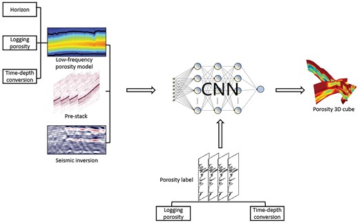
The workflow of the proposed porosity prediction strategy incorporating the constraint of low-frequency porosity model.
2.2. Low-frequency porosity model building
The construction of the low-frequency model directly from logging porosity involves three main steps: frame table construction, interpolation, and filtering. First, a stratigraphic framework is established by stacking successive stratigraphic layers, which serve as the base map. Logging porosity curves are later interpolated within this framework, resulting in the incorporation of some structural continuity into the final low-frequency porosity model. Next, the inverse distance weighting interpolation method is utilized to interpolate the porosity logging curve based on the solid model and the time-depth conversion. This method improves on distance-weighted interpolation by assigning greater weight to closer points and smaller weight to farther points, enabling more accurate estimation of attribute values for unknown points (as shown in Equations (1) and (2)). Following the interpolation process, different cutoff frequencies are determined based on field data, and a low-pass filtering operation is applied to the constructed 3D porosity interpolation model. It is necessary to point out that this interpolation method, which relies solely on logging data, does not fully utilize the seismic information. But our proposed method takes advantage of geostatistical modeling results, and also fully makes use of multi-seismic information (prestack seismic gathers and inversion results).
Here, |${S}_0$| is the place without porosity value and |${S}_i$| is the ith point with porosity value. |$Z({S}_0)$| the predicted result at |${S}_0$|, |$Z({S}_i)$| the measured result at |${S}_i$| (porosity values at well position); |${w}_i$| presents the weights of the individual measurement points during the calculation process, which is calculated by equation (2); |${d}_i$| is the distance between the predicted point and each known point; and p is the exponent value that represents the influence of the known value on the predicted value, decreasing exponentially with increasing distance.
2.3. CNNS and the architecture of neural networks
CNNs are powerful and widely used machine learning algorithms, initially introduced by Yann LeCun in the 1990s (LeCun et al.1998). CNNs leverage convolutional filters to scan input data and extract meaningful features at different spatial scales. These features undergo nonlinear activation functions and pooling layers to reduce data dimensionality and facilitate further processing.
Convolutional layers utilize filters to scan input data, capturing spatial patterns, while pooling layers downsample the output of convolutional layers, reducing feature map dimensionality for subsequent layers. This process helps combat overfitting and enhance generalization. Additionally, CNNs benefit from parameter sharing, where the same filters are used across different input regions. This approach reduces the network's parameter count, improving training efficiency and reducing the risk of overfitting. Overall, convolutional layers, pooling layers, and parameter sharing contribute to the effectiveness of CNNs in feature extraction.
Figure 2 illustrates the network structure used during model training. Our network takes the prestack seismic angle gather, seismic inversion results, and low-frequency porosity model as inputs. The timestep hyperparameter significantly influences the model's prediction ability. The network structure consists of three parts of inputs: the prestack angle gather, the seismic inversion results, and low-frequency porosity model. These parts utilize different timestep values, with the prestack angle gather having the timestep of 7 ms while the seismic inversion results and low-frequency porosity model have the timestep of 19 ms, which has been determined suitable through testing. Each part comprises two convolutional layers with 128 and 64 convolution kernels, respectively. The convolution kernel sizes for the three input parts are (3, 4), (3, 2), and (3,1), and the remaining hyperparameter settings, tuned using NNI, are presented in Table 1.
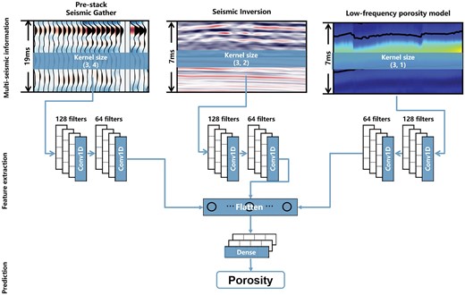
Network architecture for porosity prediction from prestack seismic data constrained by low-frequency reservoir model.
Hyperparameter settings of the network.
| Hyperparameters | Settings |
|---|---|
| Activation function | Adam |
| Optimizer | rectified linear activation function (Relu) |
| EarlyStopping patience | 60 |
| ReduceLROnPlateau patience | 30 |
| ReduceLROnPlateau factor | 0.3 |
| Hyperparameters | Settings |
|---|---|
| Activation function | Adam |
| Optimizer | rectified linear activation function (Relu) |
| EarlyStopping patience | 60 |
| ReduceLROnPlateau patience | 30 |
| ReduceLROnPlateau factor | 0.3 |
3. Geological background and data description
The data used in this study is obtained from a gas field in Sichuan Basin, SW China, which is a reef-flat carbonate (mainly dolostone) reservoir with strong heterogeneities and complex pore structures. The study area is located in the marginal facies belt of the continental shelf's eastern side. It has undergone several significant tectonic events, resulting in distinct phases of structural deformation in the region.
Figure 3 illustrates the post-stack seismic records (fig. 3a) and seismic inversion results, including P-impedance (fig. 3b) and Vp/Vs ratio (fig. 3c), crossed eight wells (W15, W3, W19, W18, W1, W2, W8, W7) in the study area. There are three formations in the study area, which are H1, H2, and H3 from top to bottom. According to the drilling and seismic interpretation result, the primary target carbonate reservoir mainly composed of dolostone is located in the H2 formation (the second column of fig. 2). The seismic inversion results (P-impedance and Vp/Vs ratio) are obtained using the prestack AVO (amplitude-versus-offset) inversion method based on the Fatti Modification of Aki–Richards equation, which is a linear approximation from Zoeppritz equations. (Fatti et al.1994). The whole prestack AVO inversion is implemented using a commercial software with strict quality control. The distribution of well locations in the study area is presented in fig. 4, where a total of 19 wells are located, with four of them having shear wave velocity measurements. Figure 5 shows the crossplots of P-impedance and Vp/Vs ratio against porosity, where the relationship between porosity and those two elastic parameters is very scattered and highly nonlinear. As can be clearly seen in fig. 5a, although the P-impedance overall decrease with porosity, at the given porosity, the P-impedance can vary significantly. This is likely caused by the heterogeneous pore structure (e.g. dissolved cavities, intercrystalline pores, and cracks) occurring in the dolostone reservoir complicating the velocity-porosity relationship. Figure 5c shows the crossplot of P-impedance and Vp/Vs ratio colored by porosity. It is apparent that the Vp/Vs ratio shows much weaker sensitivity to porosity than that of P-impedance. As a consequence, porosity prediction solely using traditional inverted elastic parameters is very challenging.
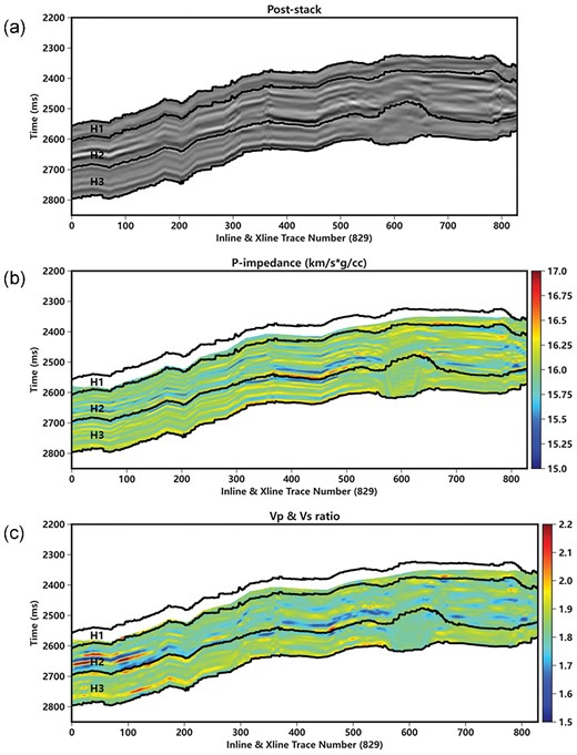
The (a) poststack seismic records and prestack seismic inversion results, (b) P-impedance, and (c) Vp/Vs ratio) in the study area.
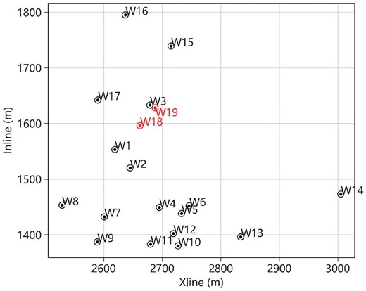
The locations of the wells used in this study.
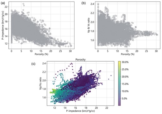
Crossplots between (a) P-impedance and porosity, (b) Vp/Vs ratio and porosity, and (c) P-impedance and Vp/Vs ratio colored by porosity.
Figure 6 displays the lithology, porosity, prestack seismic angle gather, inverted Zp (P-impedance), and inverted Vp/Vs ratio at the location of well W14. It is evident that regions with high and low porosity predominantly correspond to dolomite. Owing to variations in data acquisition methods, logging and seismic data have different scales. Therefore, to establish porosity labels (the third column of fig. 6), we initially utilize the time-depth relationship to convert the porosity well log curves from depth domain to time domain. Subsequently, we downsample the curves to ensure that they have the same sampling interval as the seismic data.
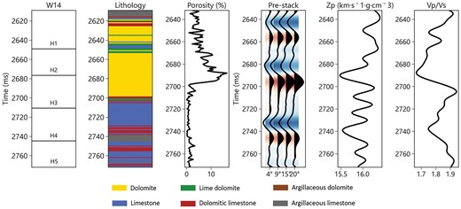
The geological background and labeled data of W14. From left to right: formation, lithology, porosity, prestack seismic angle gather, inverted Zp, and inverted Vp/Vs ratio.
4. Results
4.1. Low-frequency porosity model
During the establishment of the low-frequency porosity model, we applied a low-pass filter to the interpolated porosity volume, using a cutoff frequency of 20 Hz (the impact of different frequencies will be discussed in subsequent sections). From the constructed 3D low-frequency porosity model, we extracted the low-frequency curve of porosity at the well location along the well trajectory. Figure 7 displays the low-frequency porosity model curve at the well location, with the true porosity value represented by the black solid line, and the low-frequency porosity model value depicted by the orange dashed line. It is evident that the low-frequency curve captures very smooth variation trends in porosity.

The low-frequency porosity model curve at the well location.
4.2. The influences of the low-frequency constraint on porosity prediction
After constructing the low-frequency porosity model, we investigate the effects of low-frequency constraints on porosity prediction. In this experiment, we randomly selected four wells from a set of 17 as “blind wells,” while the remaining 13 wells were used for training. The input features for the network included prestack seismic gather, seismic inversion results (P-impedance and Vp/Vs ratio), and the low-frequency porosity curve. We conducted 100 tests, each time with different randomly selected well combinations, resulting in 100 different sub-models. Figure 8 illustrates the visualization of the prediction results for two randomly selected sub-models out of the 100 experiments. The purpose is to highlight the impact of the low-frequency constraint by comparing the porosity prediction performance of the model with and without the low-frequency constraint. Figure 8 parts a and b present the prediction results for group 34 (W11, W6, W14, W17) and group 72 (W5, W2, W9, W17), respectively. The light blue dashed line represents the predicted results using our proposed strategy, the dark blue dashed line represents the predicted results using pure data-driven prediction without the low-frequency constraint, and the black solid line represents the true label.
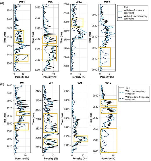
The prediction results for (a) group 34 and (b) group 72 in random experiments illustrate the constraints of low-frequency porosity model. The light blue dashed line represents the predicted results using our proposed strategy, the dark blue dashed line represents the predicted results using pure data-driven prediction without the low-frequency constraint, and the black solid line represents the true label.
As we can see, the incorporation of the low-frequency constraint has led to a significant improvement in the overall porosity prediction performance. In particular, the trained model with the low-frequency constraint demonstrates a better ability to capture the variation trend of porosity. The depth range highlighted by the orange frame indicates where the prediction performance has been notably improved with the incorporation of the low-frequency porosity model. On the other hand, within the supervised CNN framework, pure data-driven predictions without the low-frequency constraint will result in substantial prediction errors. For instance, in the two high-porosity areas (2540–2550 and 2560–2580 ms) of well W6, pure data-driven models failed to capture the underlying relationship, which will mislead subsequent reservoir characterization. Moreover, by comparing the performance of two sub-models both trained with two different training data sets on W17, it is interesting to notice that the prediction performance behaves differently when the training data set is altered. This demonstrates the high dependence of the model prediction ability on the labeled training data. However, in both cases, even when the labeled training data changes, the incorporation of the low-frequency porosity model can still significantly enhance the porosity prediction performance.
Furthermore, we calculate the RMSE of the blind test from the 100 random experiments. As shown in fig. 9, The dark blue line represents the deep learning model without low-frequency information, while the light blue line represents the model with low-frequency information. The statistical results illustrate that, after incorporating low-frequency constraint, the prediction errors in the 100 experiments are significantly lower compared to those without low-frequency constraint. Additionally, we averaged the RMSE over the 100 random trials, as demonstrated in fig. 10. It shows that after adding low-frequency constraint, the average RMSE error decreased from 4.09 to 2.66%, representing a reduction of ∼40%. Therefore, it can be concluded that low-frequency reservoir model can improve the prediction ability of the network model.
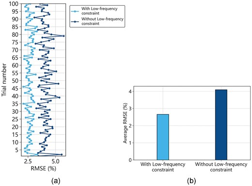
Statistical results (RMSE) of 100 random trials. (a) Statistical results (RMSE) of every trial, the dark blue line represents the machine learning model without low-frequency information, while the light blue line represents the model with low-frequency information. (b) The average error statistics of 100 trials.
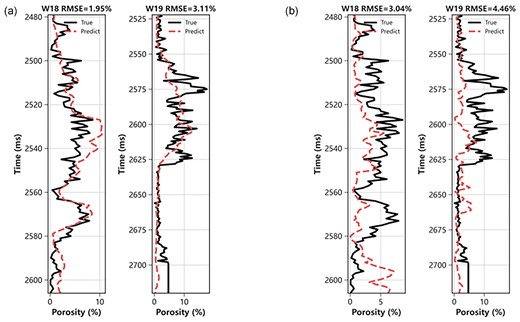
Porosity prediction result of blind wells (W18 and W19). (a) The result predicted by a model with low-frequency constraint. (b) The result is predicted by a model without low-frequency constraint.
Also, it is observed that the prediction errors vary among different sub-models, which is related to changes in the training samples. The dark blue and light blue curves exhibit similar trends, but the degree of fluctuations in the light blue curve is lower than that of the dark blue curve (fig. 9). This further suggests that, to a certain degree, incorporating low-frequency background trends can mitigate the uncertainty arising from the quality of the labeled training data.
4.3. Blind test for porosity prediction
In this section, we evaluate the generalization ability of the network model through blind testing on two wells, W18 and W19, which are not included in the construction of the low-frequency porosity model. The training data for the network training is derived from wells W1 to W17. The low-frequency porosity models for wells W18 and W19 are based on the 3D interpolated porosity model at their respective locations.
Figure 10a presents the prediction results with the inclusion of low-frequency information, while fig. 10b displays the prediction results without low-frequency information. The black line represents the true porosity values, and the red line represents the predicted porosity values by the model. It is evident that the prediction results with the incorporation of low-frequency information exhibit better agreement with the true porosity values and accurately capture the porosity variation trend. In particular, the model effectively distinguishes the high and low-porosity zones. However, fig. 10b demonstrates that when the model relies solely on seismic information, its generalization ability is inadequate, leading to inaccurate prediction results that fail to capture the porosity variation trend effectively. Moreover, we use the average of RMSE to quantify the prediction result in the blind test. As illustrated in fig. 11, it is obvious that the model incorporating low-frequency information exhibits substantially lower prediction errors for both blind wells. The inclusion of low-frequency information results in a decrease in the RMSE of ∼32% for W18 and 30% for W19.
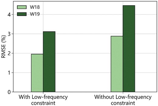
Statistical results (RMSE) of blind well testing in two wells W18 and W19 with and without low-frequency constraint.
4.4. Seismic porosity prediction with the low-frequency constraint
In this part, we present the prediction results along a profile across six training wells (W15, W3, W1, W2, W8, W7) and two blind wells (W18, W19). Figure 12 illustrates the low-frequency porosity model profile of porosity, clearly demonstrating a trend of porosity variation from low to high and then back to low throughout the reservoir. Figure 13a displays the cross-well profile of porosity prediction combined with the constraint of low-frequency porosity model.
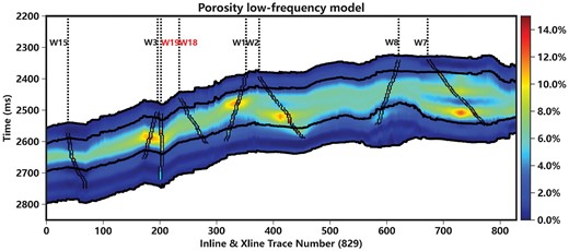
Low-frequency porosity model profile of porosity across the eight wells.
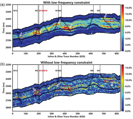
Seismic porosity prediction profile across the eight wells: (a) with low-frequency constraints and (b) without low-frequency constraints.
As we can see, the porosity prediction results on the profile align well with the well labels, such as the place indicated by the white arrows. Notably, for the two blind wells, the areas surrounding them also have good agreement with the true porosity value (white arrows), indicating the reliability of the seismic prediction results. Moreover, by comparing the low-frequency porosity model with the seismic prediction results, it can be observed that the predicted results highlighted by the yellow arrow (fig. 13a) exhibit high porosity, contrasting with the low-porosity region in the low-frequency porosity model (fig. 12). This demonstrates that the trained network model effectively captures the characteristics of seismic data and corrects the misguidance introduced by the low-frequency porosity model.
Figure 13b presents the porosity prediction section without low-frequency constraints. It is evident that the prediction results on the seismic section do not align well with the well labels. By comparing fig. 13a and b, it becomes evident that the prediction results demonstrate enhanced geological continuity after incorporating low-frequency constraints. This improvement can be attributed to the inclusion of background porosity and geological structural information during the construction of the low-frequency porosity model. Conversely, when the low-frequency constraint is omitted, the overall prediction results exhibit significant discontinuity and increased uncertainty. For instance, within the red box, in the high-porosity region between wells W3 and W19, the network effectively captures and displays the high-porosity zone when the low-frequency porosity model is employed. However, relying solely on conventional seismic information proves challenging for the model to predict this high-porosity region (the red box in fig. 13b). Similarly, the addition of the low-frequency porosity model significantly enhances the generalization capability of model in W7 and W2. Overall, the network model with low-frequency constraint that we proposed demonstrates much better predictive and generalization abilities.
5. Discussion
Different frequency band of geostatistical model contains different information concerning reservoir models. High-frequency bands usually reflect more detailed information about the reservoir model, while low-frequency bands reflect background trends. In previous experiments, we have established low-frequency porosity models with a cutoff frequency of 20 Hz, and in this section, we will discuss the impact of different frequency components of geostatistical models on the porosity prediction performance based on blind well test. In addition to 20 Hz, we also filter the model with 10, 40, 60, and 80 Hz. The porosity curves at the W1 under different cutoff frequencies are shown in fig. 14. As the cutoff frequency increases, the background trend gradually focuses on more detailed changes.
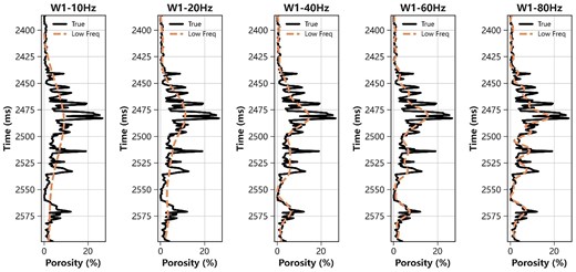
The porosity curves at the W1 under different cutoff frequencies. Here from left to right are 10, 20, 40, 60, and 80 Hz. The black line represents the true value of porosity and the orange dash line represents the low-frequency curve of porosity.
To test the effect of different frequency components on the model prediction ability, we still use the W18 and W19 as blind wells to test the prediction performance. As shown in fig. 15, for the overall error of the blind test under different frequency constraints, the network model exhibits optimal performance under the 20 Hz constraint. Also, it can be noted that the background trends of different frequencies are all effective and it is evident that overall low-frequency background trends are more effective than high-frequency constraints. Therefore, it is suitable to establish a generalized and stable model through relatively low-frequency background constraints, even if there are subtle differences in different low frequencies. It is necessary to point out that, for different geological circumstances, the most effective low-frequency reservoir model can vary accordingly. It should be tested and then selected based on the prediction performance, such as a blind test.
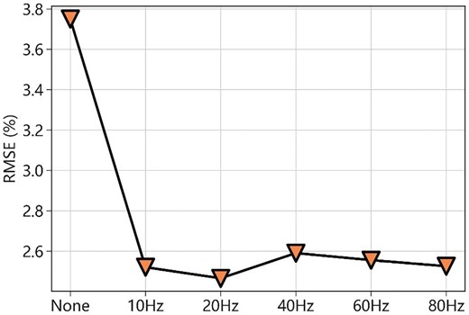
Statistical RMSE of blind test under the constraints of different frequency components of the reservoir model.
6. Conclusion
Under the supervised CNN, we propose to incorporate the low-frequency reservoir model into the deep learning framework to predict porosity from prestack seismic angle gather and seismic inversion results. With the guidance of horizon, a three-dimensional low-frequency porosity model is constructed using the inverse distance weighting interpolation method based on porosity logging curve. We demonstrate that the incorporation of low-frequency reservoir model into network training can significantly improve the porosity prediction performance. In particular, the overall porosity variation trends can be better characterized since the low-frequency information has been effectively compensated. We also test the workflow for two blind wells, where the RMSE of porosity prediction has been decreased by 34% by incorporating the constraint of low-frequency porosity model. Furthermore, the cross-well seismic porosity prediction results show that the low-frequency constraint significantly enhances the geological continuity of the porosity distribution, offering more geologically reasonable insights for carbonate reservoir characterization. The proposed method also has the potential to be extended for other reservoir parameters (e.g. clay content, saturation) prediction from seismic data.
Acknowledgements
This work was supported by the National Science Foundation of China (grant no. U20B6005), Fundamental Research Funds for the Central Universities, and Shanghai Rising-Star Program (grant no. 21QA1409200).
Conflict of interest statement. None declared.
