DenInv3D: a geophysical software for three-dimensional density inversion of gravity field data

Abstract

1. Introduction

Density is one of several key physical parameters in geophysical research. Measurements of the gravity field are the data that are most sensitive to density inhomogeneity. Density distributions can be inferred from gravity field data; such data are widely applied in the study of the geophysical exploration and Earth’s internal structure, as well as for other purposes.

Inversion of the geophysical potential field represents an ill-posed problem with non-unique solutions; thus, a number of inversion algorithms have been designed to estimate 3D density structures from gravity field data. Examples of these inversion algorithms include the damped least squares algorithm (Bear et al1995), the depth-weighted smoothing algorithm (Li and Oldenburg 1996), the Euler deconvolution algorithm (Zhang et al2000), the regularised focusing algorithm (Zhdanov et al2004), the nonlinear conjugate gradient algorithm (Commer 2011), the planted anomalous density algorithm (Uieda and Barbosa 2012), and the algebraic reconstruction technique (Li et al2016). These algorithms have rarely been implemented as software. A few softwares that perform inversions of gravity field data are available, such as Oasis montaj, ModelVision (which employs the Euler deconvolution algorithm) and GRAV3D (which employs the depth-weighted smoothing algorithm). Compared with the algorithms in these softwares, the PCG algorithm utilizes only the first derivative of the function, requires less computer memory, and has a faster convergence rate; thus, the PCG algorithm is more suitable for solving large-scale problems.

This paper presents the Matlab-based software DenInv3D, which uses the improved PCG algorithm to perform density inversions using gravity field data. The operation process is simplified in this software to make the inversion calculations more practical. Moreover, three main improvements were made to the inversion method to improve the applicability of the software. (1) Unequally spaced inversion grids are composed of rectangular prisms with different sizes in different layers, and such grids can be constructed flexibly. This method enables users to change the resolution at particular depths depending on the actual situation. (2) The regularisation parameter can be effectively determined from the inflection point of the L-curve in the PCG algorithm. (3) An established non-singular expression based on the special integration method is used to calculate the kernel function (Shu et al2015).

We constructed different synthetic models to test the utility of the software and ensure the reliability of the application when it is applied to diverse observed data. Then using the software with the improved algorithm, we obtained the distribution of anomalies on Australian Kauring test site.

2. PCG algorithms

2.1. Fundamental equations

The inverse problem is posed in the data space, leading to a linear system of equations with dimensions based on the number of data (Pilkington 2009). In general, after dividing the study area into prisms, the gravity or gravity gradient of each observation point at surface are the sum of the gravity or gravity gradient effects produced by all the underground prisms in the study area. The kernel matrix can be served as the linear projection operator from each underground prism to each observation point. Therefore, linear equations can be established between observation points and underground prisms, linear forward calculations can be performed to describe the gravity field and density distribution. We seek a model objective function that enables us to account for prior information. Thus, the constructed model align with both the observations and the additional geophysical constraints (van Decar and Snieder 1994). Therefore, the PCG algorithm was adopted to solve the linear equations.

The equation | ${\boldsymbol{d}}={\boldsymbol{Gm}}$ |$\mathit{d}=\mathit{Gm}$ can be used to express gravity field data, where | ${\boldsymbol{m}}={({m}_{{\rm{1}}},{m}_{{\rm{2}}},\mathrm{...},{m}_{N})}^{{\rm{T}}}$ |$\mathit{m}={(m_{\mathrm{1}},m_{\mathrm{2}},\mathrm{...},m_N)}^{\mathrm{T}}$ is the model parameter vector, | ${\boldsymbol{d}}={({d}_{{\rm{1}}},{d}_{{\rm{2}}},\mathrm{...},{d}_{M})}^{{\rm{T}}}$ |$\mathit{d}={(d_{\mathrm{1}},d_{\mathrm{2}},\mathrm{...},d_M)}^{\mathrm{T}}$ is the observed gravity or gravity gradient, and the kernel matrix G with M rows and N columns is the linear projection operator from the model space to the observation space. Solving for the model parameter vector m can provide the solution for the linear equation | ${\boldsymbol{d}}={\boldsymbol{Gm}}.$ |$\mathit{d}=\mathit{Gm}.$ This equation is a highly underdetermined problem and the solution can only be found by incorporating adequate prior information into the inversion equations.

Occam’s inversion method, proposed by Constable et al (1987) and DeGroot-Hedlin and Constable (1990), was employed in this study. Occam’s inversion method can be expressed with the objective function:

$\text{Missing begin{equation} or extra end{equation}}$

$\mathrm{minimize}:\varphi ={\varphi }_d+\mu {\varphi }_m,$

1

where | $\mu $ |$\mu$ is the regularisation parameter, | ${\phi }_{d}$ |${\varphi }_d$ is the observed data misfit, and | ${\phi }_{m}$ |${\varphi }_m$ is the model objective function. The regularisation parameter is a trade-off factor between the data misfit for the given data and the the model objective function.

$\text{Missing begin{equation} or extra end{equation}}$

${\varphi }_d={{\displaystyle \sum _{i=1}^N\left({\displaystyle \frac{\mathrm{\Delta }{\mathit{d}}_i-{\mathit{G}}_i\mathrm{\Delta }\mathit{m}}{{\sigma }_i}}\right)}}^2={\parallel {\mathit{W}}_d(\mathrm{\Delta }\mathit{d}-\mathit{G}\mathrm{\Delta }\mathit{m})\parallel }^2,$

2

where | ${\rm{\Delta }}{\boldsymbol{m}}={\boldsymbol{m}}-{{\boldsymbol{m}}}_{0}$ |$\mathrm{\Delta }\mathit{m}=\mathit{m}-{\mathit{m}}_0$ is the modification of model parameter vector m from the initial model m₀. The initial model may be a general background model that is obtained from previous investigations, such as other geophysical surveys, or it could also be the zero model. The initial model would generally be included in but can be removed if desired from any of the remaining terms (Li and Oldenburg 1996). The initial model always serves as the initial value in the whole inversion calculation. | ${\rm{\Delta }}{\boldsymbol{d}}$ |$\mathrm{\Delta }\mathit{d}$ is the corresponding modification of the observation. | ${\sigma }_{i}$ |${\sigma }_i$ is the standard deviation of the error associated with the ith observation.

The weighted matrix W_d is defined as:

$\text{Missing begin{equation} or extra end{equation}}$

${\mathit{W}}_{\mathit{d}}=\mathrm{d}\mathrm{i}\mathrm{a}\mathrm{g}\{1/{\sigma }_1,1/{\sigma }_2,\mathrm{...},1/{\sigma }_N\}.$

3

The principle of the inversion method is to identify m such that | $\phi \to \,\min ,$ |$\varphi \to \min ,$ under the condition of fitting the observations.

2.2. Regularisation parameter

The original regularisation parameter in Occam’s inversion method is the Lagrange multiplier. In large-scale problems, it is difficult to determine the value of this operator. As this method tends to identify several operator values that satisfy the data misfit constraint for a given small initial value, one of the values that satisfy | $\phi \to \,\min $ |$\varphi \to \min$ must be selected as the regularisation parameter. In general, because this process requires a series of calculations, empirical values are typically used to set the values of some parameters. Selecting empirical values of parameters for diverse observed data sets introduces uncertainty into the results, which weakens the applicability of Occam’s inversion method.

The L-curve is a log–log plot of the norm of a regularised solution versus the norm of the corresponding residual norm (Hansen 1992). It is effective for assessing the trade-off between the model objective function and the data misfit, which should both be controlled. When these two functions are plotted versus each other as a curve parameterised by the regularisation parameter, there is one obvious inflection point on the L-curve. When the value of the regularisation parameter is larger than the value of the inflection point, the curve will not fit the model objective well, and the data misfit will be too large. When the value of the regularisation parameter is smaller than the value of the inflection point, the data misfit is of little significance. In such cases, the solutions will be dominated by the contributions from the model objective function, and they will be over-smoothed. The value of the inflection point of the L-curve is taken to be the optimal regularisation parameter.

The inflection curvature of L-curve is defined as (Hansen 1992):

$\text{Missing begin{equation} or extra end{equation}}$

$k={\displaystyle \frac{\stackrel{⌢}{\rho }\prime \stackrel{⌢}{\eta }″-\stackrel{⌢}{\rho }″\stackrel{⌢}{\eta }\prime }{{[{(\stackrel{⌢}{\rho }\prime )}^2+{(\stackrel{⌢}{\eta }\prime )}^2]}^{3/2}}},$

4

where | $\mathop{\rho }\limits^{\frown {}}=\,\mathrm{log}({\phi }_{d}),$ |$\stackrel{⌢}{\rho }=\log ({\varphi }_d),$| $\mathop{\eta }\limits^{\frown {}}=\,\mathrm{log}({\phi }_{m}),$ |$\stackrel{⌢}{\eta }=\log ({\varphi }_m),$ and the symbols ′ and ″ represent the first and second derivatives of the function, respectively. Therefore, identifying the maximum curvature of the L-curve is considered to be the value of the regularisation parameter in the inversion process as a whole.

2.3. Model roughness

To construct the model objective function, the model roughness of Occam’s inversion method helps us to identify a smooth model that agrees reasonably well with the observations. The model roughness is useful for identifying profiles of the inversion results, which are continuous in three directions.

The model roughness is defined as (Constable et al1987):

$\begin{array}{ccc}R\hfill & =\hfill & {\parallel {\partial }_x\mathrm{\Delta }\mathit{m}\parallel }^2+{\parallel {\partial }_y\mathrm{\Delta }\mathit{m}\parallel }^2+{\parallel {\partial }_z\mathrm{\Delta }\mathit{m}\parallel }^2\hfill \\ \hfill & =\hfill & {{\displaystyle \int \left(\frac{\partial \mathrm{\Delta }\mathit{m}}{\partial x}\right)}}^2\mathrm{d}v+{{\displaystyle \int \left(\frac{\partial \mathrm{\Delta }\mathit{m}}{\partial y}\right)}}^2\mathrm{d}v\hfill \\ \hfill & \hfill & +{{\displaystyle \int \left(\frac{\partial \mathrm{\Delta }\mathit{m}}{\partial z}\right)}}^2\mathrm{d}v\hfill \end{array}$

5

| $\parallel \mathrm{...}\parallel $ |$\parallel \mathrm{...}\parallel$ denotes the usual Euclidean norm. Substituting the differential with the infinite difference, the model roughness R can be expressed in matrix form:

$\text{Missing begin{equation} or extra end{equation}}$

$\mathit{R}=\mathrm{\Delta }\mathit{m}({\mathit{R}}_x^{\mathrm{T}}{\mathit{R}}_x+{\mathit{R}}_y^{\mathrm{T}}{\mathit{R}}_y+{\mathit{R}}_z^{\mathrm{T}}{\mathit{R}}_Z)\mathrm{\Delta }\mathit{m}.$

6

2.4. Depth weighting function

There is no depth resolution associated with gravity field data (Li and Oldenburg 1998). Moreover, at a certain point, the data are inversely proportional to the distance from the source to the observed point, and the kernel function declines rapidly with depth. These properties suggest that the density distribution tends to concentrate near the surface, despite the true depth of the anomalies. A depth weighting function was added to the model objective function to counteract the natural decay of the kernel function and to overcome the tendency of density to concentrate at the surface.

Li and Oldenburg (1996) introduced the depth weighting function:

$\text{Missing begin{equation} or extra end{equation}}$

$W(z)={\displaystyle \frac{1}{{(Z+Z_0)}^{\beta /2}}},$

7

where Z is the block unit depth, β is usually equal to 2 for gravity data and 3 for gravity gradient data, and Z₀ depends on the observation height and the cell size of the model discretization.

2.5. The PCG algorithm

The objective function is required to include terms that penalise discrepancies from a initial model, and the incorporated model roughness make the model smooth in the three spatial directions. The depth weighting function was used to distribute the density with depth in the model objective function. The objective function is:

$\begin{array}{ccc}{\varphi }_m(\mathit{m})\hfill & =\hfill & {\alpha }_s{\displaystyle {\int }_V{(\partial \mathit{W}(z)\mathrm{\Delta }\mathit{m})}^2}\mathrm{d}v+{\alpha }_x{\displaystyle {\int }_V{\left(\frac{\partial \mathit{W}(z)\mathrm{\Delta }\mathit{m}}{\partial x}\right)}^2}\hfill \\ \hfill & \hfill & \times \mathrm{d}v+{\alpha }_y{\displaystyle {\int }_V{\left(\frac{\partial \mathit{W}(z)\mathrm{\Delta }\mathit{m}}{\partial y}\right)}^2}\mathrm{d}v+{\alpha }_z{\displaystyle {\int }_V{\left(\frac{\partial \mathit{W}(z)\mathrm{\Delta }\mathit{m}}{\partial z}\right)}^2}\hfill \\ \hfill & \hfill & \times \mathrm{d}v,\hfill \end{array}$

8

where | ${\alpha }_{s},{\alpha }_{x},{\alpha }_{y},{\alpha }_{z}$ |${\alpha }_s,{\alpha }_x,{\alpha }_y,{\alpha }_z$ are coefficients that affect the relative weights of the different components of the objective function.

The model is made into discrete quantities according to the specified grid. When the differential is changed to the infinite difference, equation (8) can be expressed as the following matrix:

$\begin{array}{ccc}{\varphi }_m(\mathit{m})\hfill & =\hfill & \mathrm{\Delta }{\mathit{m}}^{\mathrm{T}}({\mathit{W}}_s^{\mathrm{T}}{\mathit{W}}_s+{\mathit{W}}_x^{\mathrm{T}}{\mathit{W}}_x+{\mathit{W}}_y^{\mathrm{T}}{\mathit{W}}_y\hfill \\ \hfill & \hfill & +{\mathit{W}}_z^{\mathrm{T}}{\mathit{W}}_z)\mathrm{\Delta }\mathit{m}\hfill \\ \hfill & =\hfill & \mathrm{\Delta }{\mathit{m}}^{\mathrm{T}}{\mathit{W}}_i^{\mathrm{T}}{\mathit{W}}_i\mathrm{\Delta }\mathit{m}.\hfill \end{array}$

9

The model weighting matrix | ${{\boldsymbol{W}}}_{i}$ |${\mathit{W}}_i$ incorsporates the coefficients | ${\alpha }_{s},{\alpha }_{x},{\alpha }_{y},{\alpha }_{z},$ |${\alpha }_s,{\alpha }_x,{\alpha }_y,{\alpha }_z,$ the depth weighting function and the model roughness.

$\text{Missing begin{equation} or extra end{equation}}$

${\mathit{W}}_{\mathit{i}}={\alpha }_i{\mathit{R}}_i\mathit{D},(i=s,x,y,z),$

10

where R_i is the finite-difference operator of the model roughness and D is the diagonalization matrix of the discretized depth weighting.

Substituting equation (9) and the observed data misfit into equation (1),

$\text{Missing begin{equation} or extra end{equation}}$

$\varphi ={(\mathit{d}-\mathit{G}\mathrm{\Delta }\mathit{m})}^{\mathrm{T}}(\mathit{d}-\mathit{G}\mathrm{\Delta }\mathit{m})+\mu \mathrm{\Delta }{\mathit{m}}^{\mathrm{T}}{\mathit{W}}_i^{\mathrm{T}}{\mathit{W}}_i\mathrm{\Delta }\mathit{m}.$

11

Equation (11) can be expressed as the following matrix:

begin{eqnarray}\left[$$\begin{array}{l}\mathit{G}\\ \sqrt{\mu }{\mathit{W}}_i\end{array}$$\right]{\rm{\Delta }}{\boldsymbol{m}}=\left[$$\begin{array}{l}\mathit{d}\\ 0\end{array}$$\right].\end{equation}

$\left[\begin{array}{c}\mathit{G}\hfill \\ \sqrt{\mu }{\mathit{W}}_i\hfill \end{array}\right]\mathrm{\Delta }\mathit{m}=\left[\begin{array}{c}\mathit{d}\hfill \\ 0\hfill \end{array}\right].$

12

Set

${\boldsymbol{A}}=\left[$$\begin{array}{l}\mathit{G}\\ \sqrt{\mu }{\mathit{W}}_i\end{array}$$\right]$

$\mathit{A}=\left[\begin{array}{c}\mathit{G}\hfill \\ \sqrt{\mu }{\mathit{W}}_i\hfill \end{array}\right]$ as the Jacobian matrix,

${\boldsymbol{b}}=\left[$$\begin{array}{l}\mathit{d}\\ 0\end{array}$$\right];$

$\mathit{b}=\left[\begin{array}{c}\mathit{d}\hfill \\ 0\hfill \end{array}\right];$ equation (12) can be denoted as:

$\text{Missing begin{equation} or extra end{equation}}$

$\mathit{Am}=\mathit{b}.$

13

In addition, | ${{\boldsymbol{A}}}^{{\rm{T}}}{\boldsymbol{A}}=({{\boldsymbol{G}}}^{{\rm{T}}}{\boldsymbol{G}}+{\mu }^{-1}{{\boldsymbol{W}}}_{i}^{{\rm{T}}}{{\boldsymbol{W}}}_{i}).$ |${\mathit{A}}^{\mathrm{T}}\mathit{A}=({\mathit{G}}^{\mathrm{T}}\mathit{G}+{\mu }^{-1}{\mathit{W}}_i^{\mathrm{T}}{\mathit{W}}_i).$ To prevent excessive convergence and to increase the stability of the solution, the normal equation (13) can be modified as follows:

$\text{Missing begin{equation} or extra end{equation}}$

$\mathit{S}{\mathit{A}}^{\mathrm{T}}\mathit{Am}=\mathit{S}{\mathit{A}}^{\mathrm{T}}\mathit{b},$

14

where S is the preconditioned matrix, which is approximately equal to | ${({{\boldsymbol{A}}}^{{\rm{T}}}{\boldsymbol{A}})}^{-1}.$ |${({\mathit{A}}^{\mathrm{T}}\mathit{A})}^{-1}.$ Hence, | ${\boldsymbol{S}}({{\boldsymbol{A}}}^{{\rm{T}}}{\boldsymbol{A}})\approx {\boldsymbol{I}},$ |$\mathit{S}({\mathit{A}}^{\mathrm{T}}\mathit{A})\approx \mathit{I},$ where I is the unit matrix. If a reasonable S is selected, then the preconditioned matrix is capable of improving the number of equation conditions. The effect of the preconditioned matrix will be to concentrate the eigenvalues of the kernel function; thus, the convergence speed of the PCG algorithm is accelerated. In theory, the best choice for S is | ${({{\boldsymbol{A}}}^{{\rm{T}}}{\boldsymbol{A}})}^{-1}.$ |${({\mathit{A}}^{\mathrm{T}}\mathit{A})}^{-1}.$ However, it is unrealistic to obtain S directly in practice. In practical applications, the depth weighting function of equation (7) can be taken as the preconditioned operator (Pilkington 1997) to effectively improve the condition number of the equation. The applicability of this method has previously been demonstrated using field examples.

The PCG is an iterative algorithm for solving linear and nonlinear problems (Pilkington 2009). It is mainly used for the quadratic equation | $\phi =\tfrac{1}{2}{{\boldsymbol{m}}}^{{\rm{T}}}{\boldsymbol{Am}}-{{\boldsymbol{m}}}^{{\rm{T}}}{\boldsymbol{b}}.$ |$\varphi =\frac{1}{2}{\mathit{m}}^{\mathrm{T}}\mathit{Am}-{\mathit{m}}^{\mathrm{T}}\mathit{b}.$ The solution of this equation is | ${\boldsymbol{m}}={{\boldsymbol{A}}}^{-1}{\boldsymbol{b}},$ |$\mathit{m}={\mathit{A}}^{-1}\mathit{b},$ which is equivalent to linear equation (13). The algorithm takes the gradient at the initial point as the original conjugate direction, searches for the minimum point of the objective function in this direction and improves the stability of the solution accordingly. Moreover, the algorithm utilizes only the first derivative of the function, and its convergence rate is fast. The inversion algorithm process can be referred to Pilkington (1997) and Li and Yang (2011).

3. DenInv3D software

3.1. Main functions of DenInv3D

The DenInv3D software GUI is separated into three major independent partitions: Modelling; Calculation of the Kernel Function; and Parameter Setting, Inversion Calculation and Drawing (figure 1). The Modelling partition enables users to construct underground inversion models within particular study areas. The Calculate Kernel Function partition enables users to calculate the corresponding kernel function for gravity or gravity gradient inversion. The Parameter Setting partition contains the essential parameters of the PCG algorithm. The Calculate and Draw functions can be executed with the Calculate button and the Draw option in the menu of the DenInv3D window, respectively. The PCG source code is written in Matlab; Matlab version R2016b is required to use all of the functionality of the DenInv3D software. Figure 2 shows the flow chart of the inversion calculation in the software.

Figure 1.

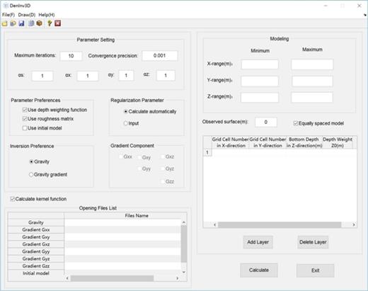
GUI of DenInv3D.

Open in new tabDownload slide

Figure 2.

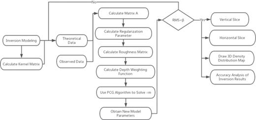
Flow chart of the inversion performed in DenInv3D.

Open in new tabDownload slide

3.2. Modelling

Within the DenInv3D interface, users first specify the boundaries for the gridded inversion model in the Modelling partition. We have adopted a right-handed Cartesian coordinate system with the z-axis pointing vertically downward. Specifying the coordinate system involves defining the X-range, Y-range, and Z-range of the model grid. Moreover, the vertical height must be specified for the observed data. To construct and display an inversion model, users first select Add Layer and input the cell numbers and thickness of each layer. The initial model starts with densities set to zero. Users can also enter initial density model files with specific values by selecting File ▷Open ▷Initial Density Model. The existing model can be imported directly in the same way. The density unit of the inversion results is the grams per cubic centimetre. Metres are used as the unit of length. Figure 3(a) shows the modelling parameter settings of the software. Figure 3(b) presents a stylized 3D view of the underground gridded model.

Figure 3.

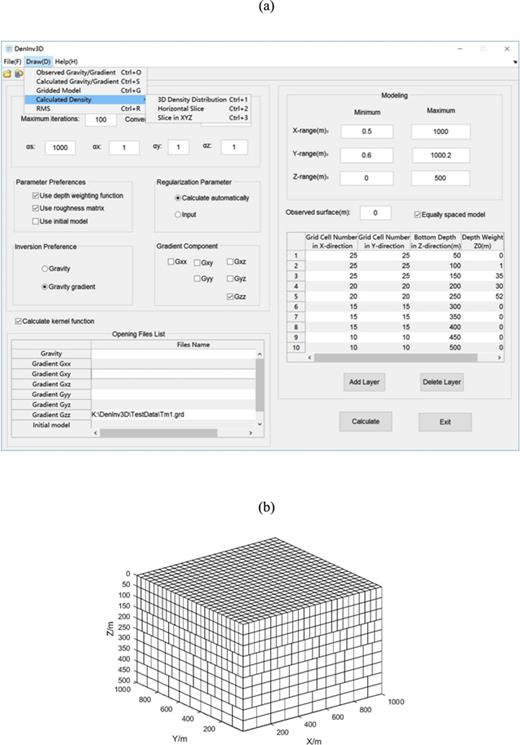
Modelling. (a) Setting values for the model; (b) constructed gridded model.

Open in new tabDownload slide

The software has the ability to construct unequally spaced model grids with considerable flexibility. Unequally spaced model grids are characterised in terms of the number of prisms in each layer. It is beneficial to build unequally spaced model grids. In particular, as depth increases, if the sizes of the deep grid cells are larger than those in the layers closer to the surface, the number of constructed prisms in each layer decreases progressively over large areas. This method aims to ameliorate the inherently ill-conditioned problems that exist in the inversion of gravity or gravity gradient data and to weaken the attenuation of the kernel function. Furthermore, the resolution of models can be changed in different layers. We adopted this method for all the inversion models in this paper.

3.3. Kernel function

The observed data must be selected from the menu File ▷Open ▷Observed gravity/Observed gradient before the kernel function is calculated. The file containing the observed data should be in a text grid with the file name extension GRD. Moreover, Gravity or Gravity Gradient under Inversion Preferences should be selected, the corresponding variables should be confirmed under Gradient Component, and Calculate Kernel Function should be selected. Analytic singular points exist in the general forward modelling expressions. To solve this problem, we adopted an established non-singular expression based on the special integration method to calculate the kernel matrix G (Shu et al2015). Users are advised to calculate the kernel matrix initially.

3.4. Parameter preferences

The Maximum iterations, the Convergence criteria and the weighting coefficients of the objective function | $({\alpha }_{s},{\alpha }_{x},{\alpha }_{y},{\alpha }_{z})$ |$({\alpha }_s,{\alpha }_x,{\alpha }_y,{\alpha }_z)$ must be entered manually. The Regularisation parameter, Depth weighting function and the Roughness matrix options are selected in the Parameter Setting partition of the GUI.

3.5. Calculation and drawing

After performing the inversion, users can save the density result in a plain data format with the file name extension .DAT. The software can calculate the gravity or gravity gradient with the density of the inversion model, the root mean square of the observed and calculated gravity or gravity gradient, which is used to evaluate the accuracy of the inversion results. The Drawing function enables users to display the inversion results. The software is capable of displaying the Observed Data, the Calculated Data, the 3D Density Distribution, the Slice in XYZ and the Horizontal Slice. Users can select the options in the Draw menu in the DenInv3D window to produce these figures.

4. Tests studies

4.1. Test of parameters

We construct different synthetic models as test models firstly, which are conducted as given models with the specific different sizes, shapes, depths and densities to test the effectiveness of the inversion calculation. To illustrate the effects of different parameters selected in our software, we used one simple prism (length × width × height: 200 m × 200 m × 200 m) as an example, as shown in figure 4(a). When we selected only the regularisation parameter and did not consider the model roughness, the results illustrated in figure 4(b) were obtained. In this case, the distribution is one thin layer of mass just beneath the surface. When we added the model roughness at the same time, the result is smooth in three spatial directions, and the sudden jump in density values is not seen in the adjacent cells, as shown in figure 4(c). Adding the depth weighting function overcomes the tendency to concentrate density at the surface, as shown in figure 4(d). The anomalies are concentrated and situated at the depth that accords with the real model. The combination of these three functions yields the best inversion results.

Figure 4.

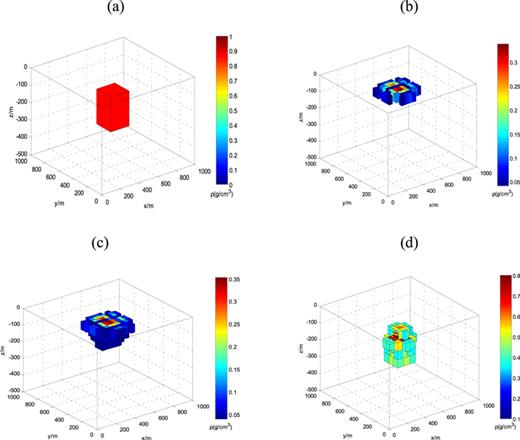
Parameter experiments. (a) Real model; (b) with the regularisation parameter added; (c) with the regularisation parameter and the roughness model added; (d) with the regularisation parameter, the roughness model and the depth weighting function added.

Open in new tabDownload slide

4.2. Test of synthetic models

To test the utility of the software and ensure the reliability of the application when it is applied to diverse observed data, we constructed three different synthetic models. M1 (figure 5(a)) is a synthetic model containing two rectangular prisms with high density. Both prisms are situated at a depth of 150 m with a density contrast of 1 g cm⁻³, and the two prisms are of the same size (200 m × 200 m × 200 m). M2 (figure 5(d)) is a synthetic model containing a trapezoid and a prism. The trapezoid consists of four prisms of approximately the same size at different depths on the left (200 m × 100 m × 50 m). Another prism on the right extends along the y-axis (400 m × 100 m × 100 m). The two figures are at different depths (100 m and 150 m) and have a density contrast of 1 g cm⁻³ and 0.8 g cm⁻³, respectively. M3 (figure 5(g)) is the synthetic model of four distinct spatial geometric models. The four models have different sizes, densities and depths. We added 5% Gaussian random noise to the synthetic data, which was referred to as the ‘observed gradient data’. For the simple synthetic model M1, the inversion results are obtained with the observed gradient data T_zz, and for the complex models M2 and M3, the observed gradient data are composed of five independent gravity gradient components. The number of iterations, the calculated regularisation parameters, the modelling errors and fitting errors are listed in table 1.

Figure 5.

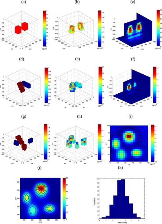
Synthetic data test. (a) Synthetic M1; (b) calculated M1; (c) vertical section of calculated M1; (d) synthetic M2; (e) calculated M2; (f) vertical section of calculated M2; (g) synthetic M3; (h) calculated M3; (i) transverse section of calculated M3; (j) contour map of the calculated component | ${{\boldsymbol{T}}}_{zz}^{{\prime} }$ |${\mathit{T}}_{zz}^{\prime }$ and the measurements T_zz; (k) histogram of residuals between the calculated component | ${{\boldsymbol{T}}}_{zz}^{{\prime} }$ |${\mathit{T}}_{zz}^{\prime }$ and the measurements T_zz.

Open in new tabDownload slide

As suggested by figures 5(b), (e), and (h), which show the calculated counterparts of figures 5(a), (d), and (g), respectively, we obtained acceptable results in terms of the positions, sizes, depths and densities of the synthetic models. The vertical and transverse sections of the calculated counterparts (figures 5(c), (f), (i)) show that the anomalies are concentrated at the same positions as in the synthetic models, which indicates the validity and correctness of the software.

We performed an accuracy analysis using the complex synthetic model M3 (figure 5(g)) and the corresponding inversion model M3 (figure 5(h)). Through verifying the inversion results m, we calculated the gradient component | ${{\boldsymbol{T}}}_{zz}^{{\prime} }.$ |${\mathit{T}}_{zz}^{\prime }.$ In figure 5(j), the colours represent the original observed data | ${{\boldsymbol{T}}}_{zz},$ |${\mathit{T}}_{zz},$ whereas the contour lines represent the calculated | ${{\boldsymbol{T}}}_{zz}^{{\prime} }.$ |${\mathit{T}}_{zz}^{\prime }.$| ${{\boldsymbol{T}}}_{zz}^{{\prime} }$ |${\mathit{T}}_{zz}^{\prime }$ is highly consistent with | ${{\boldsymbol{T}}}_{zz},$ |${\mathit{T}}_{zz},$ and the differences between them are minimal. In addition, as suggested in figure 5(k), a large fraction of the differences | ${{\boldsymbol{T}}}_{zz}-{{\boldsymbol{T}}}_{zz}^{{\prime} }$ |${\mathit{T}}_{zz}-{\mathit{T}}_{zz}^{\prime }$ are close to zero. These representative synthetic examples demonstrate that the software is capable of solving problems with complex anomaly induced blocks.

4.3. Field data example

The Kauring test site has been used to collect data since 2009. Figure 6 shows the test site was located approximately 115 kilometres east–northeast of the Jandakot Airfield in Perth in western Australia. The site is used to calibrate and test airborne gravity gradiometry and airborne gradiometry systems. Fugro Airborne Surveys conducted the airborne gravity gradiometry at the Kauring test site from July 2011 to February 2012 using the FALCON airborne gravity gradiometer. The total length of flight lines over the test site was 1265.3 km and the altitude of the flying plane was 80 m. Terrain correction was applied to the gravity gradient data covering the survey area. This assisted with the density inversion of underground anomalies. To highlight the anomalies situated in shallow layers, based on the results of the parameter experiments and referring to published results (Martinez and Li 2012), the matched filtering method was adopted to eliminate the effects of density anomalies at great depth.

Figure 6.

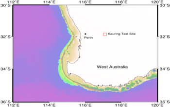
Location and topography of the Kauring gravity gradient test site.

Open in new tabDownload slide

The resolution of the airborne gradiometry data is 5.04 m, and the accuracy of the data is 5 E. Figure 7 shows the six components of the gravity gradient tensor. The subscripts n, e, and d correspond to the north-, east-, and down-axis directions of the local geographic coordinate system, respectively.

Figure 7.

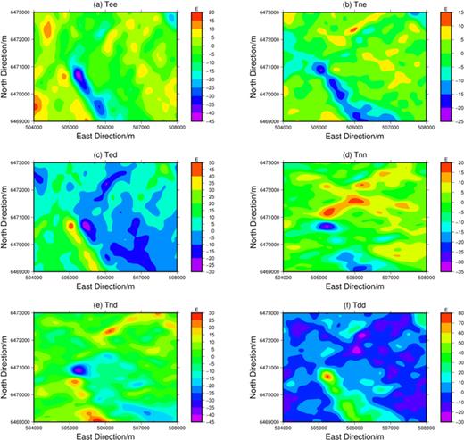
Gravity gradient tensor data obtained using a Butterworth fourth-order low-pass filter.

Open in new tabDownload slide

Using the DenInv3D software, we performed density inversion with the five independent components of the measured gravity gradient tensor. We selected 80 × 80 points to represent the observed data from each gravity gradient tensor component, and the spacing between the adjacent points was 50 m. The total number of observed points was 32 000. Using the division method of the 3D spatial model, the model was divided into ten layers, each of which had a thickness of 80 m. The horizontal dimensions of the prisms at each layer progressively increase from 80 m to 150 m with increasing depth. Therefore, there are 11 546 prisms in total, and the dimensions of the kernel matrix are 32 000 × 11 546.

Figure 8(a) shows the 3D density structure of the inversion results. To emphasise the key features, only density anomalies that are greater than 1.0 × 10³ kg m⁻³ are shown. The original point of X-range corresponds to the point at 504 000 m in east direction, the original point of Y-range corresponds to the point at 6469 000 m in north direction (figure 7). Compared with published results (e.g., Martinez and Li 2012, Liu et al2015), we discovered that anomalous blocks of different sizes are present within the study area in addition to the central anomalies. These anomalies are distributed at a certain angle, and the inferred average density of the anomalies is approximately 1.25 × 10³ kg m⁻³. Moreover, the position of the central anomaly is located at 1110–1450 m east and 1444–1890 m north. The density of the central anomaly is approximately 2.3 × 10³ kg m⁻³, which is consistent with the published results. This agreement confirms the reliability of the inversion method and the software applied to the observations.

Figure 8.

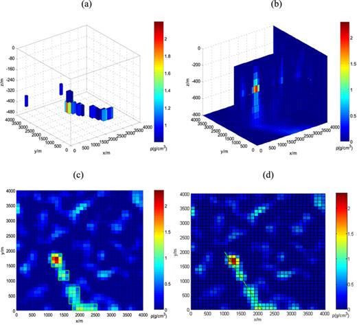
Densities estimated by inversion of gravity gradient data at the Kauring test site. (a) 3D model of the inversion results; (b) vertical section at y = 1700 m; (c) transverse section at z = 360 m; (d) transverse section at z = 360 m.

Open in new tabDownload slide

Figure 8(b) shows the vertical section at y = 1700 m, in which the central anomalies can be seen at depths ranging from 240 to 400 m. The positions of the central anomalies are consistent with those identified by Liu et al (2015), who applied anomaly depth detection methods in this area.

Figures 8(c) and (d) show a transverse section through the anomalies at a depth of 360 m. Several anomalies are distributed along a line extending from the point (2000, 0) at an angle of arctan (0.5) = 26.5°. In this transverse section, the anomalies can be seen to extend over a length of approximately 2.3 km. The dimensions of each anomaly range from 300 m × 300 m to 300 m × 500 m. The anomalies can be divided into four distinct blocks, and the central positions of each block are (1280, 1670 m), (1610, 1170 m), (1950, 500 m) and (2170, 110 m).

The test site is flat, and the central anomalies are situated at a depth of 360 m, which is close to the surface. No faults exist in this area in the published results. As the initial value of the density is 0 without any constraints, the anomalies have a maximum density up to 2.41 × 10³ kg m⁻³. Moreover, the mineral deposits within the test site have shallow burial depths; we conclude that the anomalies are caused by the presence of these deposits.

Using our inversion software with the improved algorithm, we determined the positions, dimensions and densities of these anomalies. The results provide the information needed to determine the distribution of the anomalies.

5. Conclusions

This paper describes the inversion software DenInv3D, which allows users to estimate 3D density fields using gravity or gravity gradient data. This software includes functions for modelling, calculating kernel functions, performing inversion calculations, and analysing and visualizing the results. The inversion calculations are based on the improved PCG algorithm. Due to the uncertainty of the Lagrange empirical parameter in the PCG algorithm, we used the inflection point of the L-curve as the regularisation parameter. In addition, this software allows the construction of unequally spaced model grids and inversion calculations using such grids, which permit changing the resolution of the inversion results at different depths. The kernel function is calculated using an established non-singular expression based on the special integration method. Application examples of the software to synthetic and field data showcase the validity of the software. The results show that the inversion of gravity field data with the DenInv3D software can yield geologically meaningful information. The software has the ability to obtain complete 3D distributions of density anomalies, which enables the analysis and interpretation of mineral exploration data and other geological data in geophysical engineering, studies of the internal structure of the Earth, and progress in relevant research fields.

Acknowledgments

This work was supported by the National Natural Science Foundation of China under Grant No. 41574073; the Major State Research Development Program of China under Grant No. 2016YFC0601101; R&D of Key Instruments and Technologies for Deep Resources Prospecting (the National R&D Projects for Key Scientific Instruments) under Grant No.ZDYZ2012-1-04.

References