


Abstract
We study the clustering behavior of stock return jumps modeled by a self/cross-exciting process embedded in a stochastic volatility model. Based on the model estimates, we propose a novel measurement of stock price efficiency characterized by the extent of jump clustering that stock returns exhibit. This measurement demonstrates the capability of capturing the speed at which stock prices assimilate new information, especially at the firm-specific level. Furthermore, we assess the predictability of self-exciting (clustered) jumps in stock returns. We employ a particle filter to sample latent states in the out-of-sample period and perform one-step-ahead probabilistic forecasting on upcoming jumps. We introduce a new statistic derived from predicted probabilities of positive and negative jumps, which has been shown to be effective in return predictions.
It has been established in the literature that stock prices sometimes exhibit significant discontinuities, and these discontinuities are often referred to as “jumps.” Numerous studies have demonstrated that news announcements are a primary driving force behind stock price jumps. For example, Lee (2012) discovers that days with scheduled news are more likely to experience return jumps. Jeon, McCurdy, and Zhao (2022) use textual analysis to investigate the impact of the news on jump intensities and jump size distributions. Also see recent studies by Gurkaynak, Kisacikoğlu, and Wright (2020), Baker et al. (2021), and Engle et al. (2021). However, the speed at which the news is incorporated into stock prices tends to depend on the nature of news—its complexity and level of informativeness (Loughran and McDonald 2014) and the attention of investors (Hirshleifer, Lim, and Teoh 2009).1 Therefore, for the less efficient stocks with low news-incorporation speed, new information may not be incorporated into stock prices with one single jump, but rather through a potential sequence of jumps. This motivates us to study the clustering behaviors of asset return jumps.
For a simple example, we plot daily stock prices, returns, volatility, and return jumps2 of the Ampco-Pittsburgh Corporation (NYSE: AP) in Figure 1. We can see subsequent return jumps after two earnings announcements despite the model’s assumption of constant jump intensities. This could occur if the return jump on the announcement date failed to fully absorb all the information and caused the second return jump. Additionally, it is noteworthy that variance increases during news announcements, which is consistent with the literature (Erdemlioglu and Yang 2023). Later in this article, we further show that such abnormal return originates from the jump clustering and stock inefficiency, which is robust to stock illiquidity.
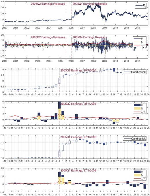
Daily price, return, jumps, and volatility of Ampco-Pittsburgh Corporation (NYSE: AP).
Notes: These variables are estimated using an SVCJ model proposed by Duffie et al. (2000) with daily data from 1 January 2000 to 31 December 2012. The last four figures are for 15 days before and 25 days after the company’s 2005Q2 and 2005Q4 earnings announcements. y denotes the stock returns, denotes the return jump component, v presents the variance.
This gives rise to the research questions we aim to address in this article: (1) What do these clustered jumps suggest? Does the information contained in the jump clustering vary across assets?; (2) Given a dependency among jumps, in the sense that jumps do not arrive independently, can we exploit this characteristic to forecast jumps? Furthermore, to what extent are these clustered jumps predictable?
In this article, we model these jumps using a self/cross-exciting point process proposed by Hawkes (1971a, 1971b). This approach enables the probability (intensity) of jumps to be dependent on past jumps. This implies that the occurrences of jumps can increase the probability of future jumps, which is in line with the jump clustering behaviors we have observed. More specifically, we separate stock return jumps into positive and negative ones. The term “self-excitation” describes the propensity for positive/negative return jumps of an asset to generate subsequent positive/negative return jumps of the same asset. Conversely, “cross-excitation” denotes the capacity for positive/negative return jumps of an asset to trigger subsequent negative/positive return jumps of the same asset. We embed the self/cross-exciting jumps in a stochastic volatility model and let the model determine whether a return includes a jump and whether additional jump clustering parameters are necessary to describe the data. We estimate the model using a Bayesian Markov Chain Monte Carlo (MCMC) method.
Based on the model, we contribute to the literature in two ways. First, we find strong evidence of jump clustering with varying degrees across assets, which are closely related to information releases. We introduce a novel measure of stock price efficiency, denoted by , based on the degree of jump clustering exhibited by asset returns. This measure is derived from the posterior distributions of the jump clustering parameters. The underlying rationale is that if a stock requires more than one jump to fully incorporate new information, it is potentially less efficient than those stocks requiring only a single jump. In light of this, assuming the arrival of information is random and independent, it stands to reason that for efficient stocks, the jump arrivals should likewise be random and independent. Thus, the extent to which a stock’s jumps cluster together can serve as a measure of its efficiency. This measure’s advantages lie in its convenience and generality. For example, one can surely assess how quickly a stock absorbs a type of information by calculating the average return drift of the stock after the information arrives. However, there are numerous types of information, and their incorporation speeds may differ. In contrast, the degree of jump clustering can be easily calculated without knowing when and what types of information arrive.
We conduct a regression analysis on cross-sectional cumulative abnormal returns (CAR) after announcements with several different stock price efficiency measures while controlling for a broad set of variables. The findings indicate that our measure, , more accurately captures the cross-sectional variations of CAR and post-earnings-announcement drifts (PEAD) compared to existing measures and is robust to control variables, including stock illiquidity.
Second, we utilize a particle filter-based framework to conduct probabilistic forecasting of return jumps. Given the presence of jump clustering and the probability of jumps being a function of past jumps, we show the possibility of forecasting the self-exciting jumps and investigating their predictability. Specifically, we first fixed static parameters at their posterior means estimated in the in-sample period. In the out-of-sample, we use a particle filter to iteratively estimate latent variables at each time point as new returns are observed. Subsequently, we approximate the predictive distribution of jumps, which is assessed by a ranked probability score (RPS). Additionally, we introduce a statistic that takes the difference between the predicted probabilities between positive and negative jumps. We find that high and low values of this statistic have predictive power on returns, with predictability directly linked to the degree of jump clustering exhibited by the asset (i.e., the stock price efficiency measure we proposed). Based on this forecasting framework, a trading strategy yields a Sharpe ratio (SR) of 1.62, inclusive of transaction costs.
Our studies contribute to several streams of literature. First, it is related to studies examining announcement effects. For example, studies on the pre-announcement drifts of macro news (Bernile, Hu, and Tang 2016; Kurov et al. 2019), PEAD (Bernard and Thomas 1989; Hung, Li, and Wang 2015), among others, show evidence of price drifts preceding and following various announcements. Moreover, Lee (2012) and Jeon, McCurdy, and Zhao (2022) relate jumps to news releases. In our article, we study the information flows from the perspective of jump clustering behaviors before and after announcements. Additionally, the findings of Christensen, Timmermann, and Veliyev (2023) based on high-frequency data indicate limited price discovery in the days following earnings announcements. However, their findings are confined to 50 liquid firms due to the extensive size of high-frequency data, while we look at all US stocks and aim to capture the speed of price discovery using daily data.
Our studies are also related to the stock price efficiency literature. The most widely used stock price efficiency measure is the price delay developed by Hou and Moskowitz (2005), who study the predictive power of lagged market returns on asset returns as a measure of stock price efficiency. Numerous studies have subsequently employed this measure. They explored the relationship between price efficiency and various factors, including short-sellings (Saffi and Sigurdsson 2011; Jones, Reed, and Waller 2016), dark trading (Foley and Putniņš 2016), share repurchase (Busch and Obernberger 2017), firm bankruptcy risk (Brogaard, Li, and Xia 2017), among others. Furthermore, Bris, Goetzmann, and Zhu (2007) propose to use the first-order autocorrelation of stock returns with lagged market returns. However, these measures predominantly capture the gradual pace at which market information is transmitted to individual assets, which is less relevant to firm-specific information. Our measurement assesses the extent to which a stock’s return jumps cluster together, without differentiating between different types of information.
Moreover, our studies contribute to the jump clustering and jump forecasting literature. The jump clustering effect is mentioned by Lee (2012) and Lee and Wang (2019). They filter jumps non-parametrically and estimate a logit model for the jump’s probability using dummy variables to capture news releases. They also include a dummy variable that equals one when there is a jump in the past period of time. They demonstrate the effectiveness of the model in forecasting the probability of jumps. Jeon, McCurdy, and Zhao (2022) also adopt a logit model of jump’s probability. In this article, we adopt a different approach. The predictability we aim to examine solely stems from the degree of jump clustering exhibited by the asset. There are also many other applications of the mutually exciting point process with financial data. For example, Aït-Sahalia, Cacho-Diaz, and Laeven (2015) investigate jump spillovers among international stock markets. Herrera and Clements (2020) develop a point process risk model that integrates a select set of covariates into the tail distribution of intraday returns. Kwok (2024) proposes a test for the dependence of jump occurrences.
Lastly, our studies are also relevant to literature on stochastic volatility models. Continuous-time stochastic volatility models have been well-established in the literature (see, e.g., Heston 1993; Bates 1996; Duffie, Pan, and Singleton 2000; Kou, Yu, and Zhong 2017). Additionally, there exists a stream a literature incorporates the self-exciting jumps into continuous-time models, for example, Maneesoonthorn, Forbes, and Martin (2017) and Chen, Clements, and Urquhart (2023). These studies concentrate on the overall fit of the model to empirical data. Furthermore, we emphasize that discrete-time stochastic volatility models also hold significant interest in the literature, particularly in modeling the cross-section of the yield curve (see, e.g., Creal and Wu 2015, 2017).
The rest of this article is organized as follows. Section 1 introduces our model. Section 2 presents model estimation approaches, the forecasting framework, and the data we used in the empirical studies. Section 3 presents our studies on news releases and stock price efficiency. Section 4 presents the out-of-sample forecasting results. Section 5 concludes the article. Some technical results are confined to the Appendix.
1. The Model
In this section, we introduce a continuous representation of an asset’s return and variance processes and how we embed a self/cross-exciting process in the model. Then, we will describe the discretized version of the model.
1.1 Return and Variance Process
Regarding the return jump component denotes the return jump size. We separate to , which follow two truncated normal distribution . denotes the variance jump size that follows an exponential distribution with mean , . The is a counting process, which is also split into with corresponding intensities . This is based on the finite activity of jumps rather than an infinite activity since our primary interest is capturing the clustering behavior of rare jumps instead of a large number of small jumps. Similarly, The is a counting process for the variance jump with corresponding constant intensity .
1.2 Self/Cross-Exciting Return Jumps
The intuition of this specification is allowing every past jump to raise up the intensity at time t, , by . In other words, when there is a jump j observed at time t, the underlying intensity will increase to instantaneously; it will decay back to by the speed of . is a matrix, capturing the self/cross-excitation (clustering) of positive and negative return jumps. Note our specification is slightly different from other literature. For example, Aït-Sahalia, Cacho-Diaz, and Laeven (2015) forgo the and let , where . can be interpreted as the incremental intensity of jumps i that is raised by past jumps j. In this case, is equivalent to in our setting.
This self/cross-excitation setup provides a model for capturing jump clustering in financial assets. allows the jump intensity to depend on past jumps. It can also be an asymmetric matrix when the extent to which positive return jumps produce negative ones is different from the extent to which negative return jumps produce positive ones. In addition, when there is no jump clustering. Indeed, this model could be expanded to higher dimensions by including the impact of jumps in all other assets. However, it is not our primary focus; we are more interested in time-series jump dependence across different assets and their predictability.
Furthermore, we define , where denotes the diagonal elements of matrix . Later in this article, we will employ to quantify an asset’s extent to which its jumps are clustering, especially those clustered jumps of the same sign. Additionally, we will explore the implications of this measure for asset pricing.
1.3 The Discretized Form
2. Bayesian Inference and Forecasting
We now introduce the in-sample estimation method and develop the out-of-sample forecasting framework. A description of the data will be provided at the end of this section.
2.1 In-Sample Estimation
We adopt a hybrid of the Metropolis–Hastings and Gibbs sampling schemes to approximate this posterior distribution. The sampling steps of self/cross-exciting parameters are given by Rasmussen (2013). A detailed specification of priors and the algorithm is provided in Appendix A.1.
2.2 Out-of-Sample Forecasting and Jump’s Predictability
Our goal in the out-of-sample is to forecast or given the information up to time t. We denote the forecasted values of as . We first fix the static parameter vector at its posterior mean estimated in the in-sample period . Then, for every return y coming in, we adopt a particle filter proposed by Pitt and Shephard (1999) to approximate the distribution of latent variables . Details of the particle filtering are provided in Appendix A.2. As a result, we will have N particles of from the particle filtering denoted as . From these estimates, we can approximate the predictive distribution , which is .3
We examine the predictive power of on y. The intuition of this statistic is capturing those times when the predicted probability of positive jumps is higher or the predicted probability of negative jumps is higher. Our focus is on how asset returns are distributed during these times.
3. Empirical Studies
3.1 Data
We primarily conduct our empirical studies on US stock data. We also examine the predictability of self-exciting jumps with 24 foreign exchange rates and 12 commodity futures data using the same forecasting framework. These results are confined to a Supplementary Appendix.
We obtain the daily US stock price data from the Center for Research in Security Prices (CRSP) for the period from 1 January 2000 to 31 December 2021. Companies’ book values data come from Compustat. We split all the stock data into in-sample and out-of-sample on 1 January 2013. We discard data before 1 January 2000 and restrict the stock to have at least 5 years of data in the in-sample to guarantee relevant and sufficient data for the Bayesian MCMC estimation. As a result, we filter out 3035 stock data.
In the Bayesian MCMC estimation, we set the number of iterations as 100,000, and the first 50,000 iterations are the burn-in period. Note that one could apply the framework with a one-year rolling window (i.e., forecast for one year and recursively re-estimate the model with the past 5 years of data). Due to the heavy computational burden, we choose not to do so, although this would likely lead to better forecast performance. Moreover, our main theme in this section is to study return jumps’ predictability across different assets rather than improve the forecasts.
To demonstrate the realized behaviors of stock return jump clustering, we first estimate a model setting all jump intensity constant (). Based on posteriors of and , we discover the following facts:
| 92.17% of stocks exhibit return jumps that occurred on their earnings announcement days at least once. |
| 44.57% of stocks exhibit, at least once, a consecutive jump following the announcement day jump. |
| 71.89% of these consecutive jumps are of the same signs as the previous jumps. |
| 62.05% of stocks have at least one jump within the subsequent four days following the earnings announcements. |
Jumps in stock prices do relate to news releases, as evidenced by earnings announcements, when over 90% of stocks exhibit at least one jump on their announcement days. This observation aligns with existing literature: the jump’s probability is significantly higher during news arrival days (see, e.g., Lee 2012; Bajgrowicz, Scaillet, and Treccani 2016; Jeon, McCurdy, and Zhao 2022; Christensen, Timmermann, and Veliyev 2023). Furthermore, this brief overview illustrates jump clustering behavior, with numerous stocks experiencing multiple jumps following earnings releases.
3.2 Jump Clustering Parameters
In the in-sample estimation, there is no need to report most of the results (posteriors of static parameters, overall model fitness, etc.) as they are not the main focus of this article. The aim is to study the posteriors of the jump clustering parameters across different assets. We remark that the information decaying speed is contained in . In addition, is a matrix capturing an expected number of jumps in i that is produced by jumps in j, where . A higher decaying speed will lead to a smaller expected number of jumps being produced. It is related to the magnitude of the incremental intensity of jumps raised by past jumps ( in the model by Aït-Sahalia, Cacho-Diaz, and Laeven (2015)). Therefore, we focus on across different assets and ignore the .
Figure 2 plots posterior means’ histograms of estimated using the US stock data from 2000 to 2012. The base-line intensities , which can also be regarded as the base-line probability of jumps, are mostly smaller than 5% representing 13 jumps in a year on average. A higher value of leads to a fatter-tailed return distribution. Therefore, this can also be an indicator of stock jump risk, which has been extensively studied in the literature (e.g., Bégin, Dorion, and Gauthier 2020). Regarding the , all four histograms exhibit evident tails, indicating that some stocks demonstrate pronounced jump clustering behaviors. However, in these four histograms, and are closer to zero compared to and , suggesting that the cross-impact of return jumps tends to be weaker than their self-excitation. Moreover, the cross-impact of return jumps could also be captured by variance jumps and variance persistence. The matrix estimated by averaging over all stocks is .5 As an arbitrary measure of parameter significance, we calculate the percentage of stocks for which the posterior means of their parameters minus 1.5 times their posterior standard deviations are greater than zero. The percentage of these four parameters is . However, we emphasize that the significance of these parameters is less likely to influence our subsequent studies.
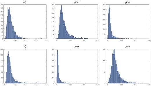
Histograms of jump clustering parameters.
Notes: These parameters are estimated using the US stock data from 1 January 2000 to 31 December 2012. We only include companies with data for more than 5 years, which results in 3035 stocks being filtered out. The jump clustering parameters for the 3035 stocks are shown by these histograms.
3.3 Characteristics of Stocks with Heavily Clustered Jumps
We have demonstrated that different assets exhibit jump clustering to varying extents indicated by jump clustering parameters. It is reasonable to ask what types of assets exhibit more pronounced self/cross-exciting jump behavior and what properties they share. To further analyze different extent of jump clustering across different assets, we define , where denotes the diagonal elements of matrix . Therefore, is simply the sum of diagonal elements in matrix . We intend to use this measure to quantify the extent to which an asset’s jumps are clustering, particularly those clustered jumps of the same sign.
We follow various traditional asset pricing papers by sorting all stocks by and forming 10 portfolios. We calculate characteristics averaged over stocks in each portfolio: market cap, book-to-market ratio, illiquidity ratio, stock market beta, idiosyncratic volatility, total volatility, and out-of-sample annualized mean return.
The table shows a clear trend across several firm characteristics. The stocks with heavier-clustered jumps are more likely associated with small market caps, higher book-to-market ratios, less trading liquidity, less sensitivity to the market factor, and higher volatility. The out-of-sample returns suggest that is potentially a pricing factor and plays a role in return prediction. But we will refrain from this viewpoint any further since it is not the focus of this article. In this section, our goal is to provide a broad overview of the characteristics of stocks whose jumps are heavily clustered. We will include the possibility of this point in future studies.
3.4 “Idiosyncratic” Stock Price Efficiency vs. Price Delays
The we proposed to measure the extent of jump clustering may also serve as a measurement of stock price efficiency. For example, if a stock requires a sequence of price jumps to absorb new information, it is potentially less efficient than a stock that only reacts with a single jump to the same information. Assuming that new information arrives randomly and that a completely efficient stock only displays one jump in response to the information, the stock price jumps should likewise arrive randomly and independently of one another. In this sense, there is no jump clustering, and of the stock will be close to zero.
These measures show some power in capturing PEAD (see Figure 1 in Hou and Moskowitz (2005)’s paper), although they are designed to measure stock delays in possessing market information instead of idiosyncratic information (e.g., earnings releases). The , on the other hand, captures the speed of possessing information regardless of whether it is macro or idiosyncratic information.
CAR double-sorted by SUE and pricing efficiency measures.
Notes: Earnings news is measured using SUE. We first categorize stocks into those with positive SUE (blue) and negative SUE (green). Stocks are sorted independently into quintiles based on the magnitude of SUE. Then, we sort stocks into quintile portfolios based on pricing efficiency measures so that each quintile contains stocks with different magnitudes of SUE but the same level of pricing efficiency. High and Low denotes the quintile portfolio with the highest and lowest pricing efficiency measures.
However, Figure 3 can be misleading if one wants to know which measure best portrays the stock price efficiency by looking at the PEAD since stocks already have different extents of drifts before the announcement, although drifts before the announcements are also valuable in several studies (see, e.g., Liu et al. 2020). Thus, we further plot Figure 4 with |CAR| |SUE| and price efficiency measures starting from the announcement dates. Note that we take CAR’s and SUE’s absolute values since their directions are insignificant in measuring price efficiency, and we care more about the magnitudes of CAR and SUE. We assume that after controlling the SUE, stocks with very high price efficiency can quickly possess the information and display modest CAR magnitudes, regardless of whether the information will lead to a positive or negative CAR. Similar to Table 1, we summarize price efficiency and PEAD measures of -sorted portfolios in Table 2.
CAR double-sorted by |SUE| and pricing efficiency measures.
Notes: These four figures are similar to Figure 3, however, we make two adjustments. First, we double-sort stocks to 10 decile portfolios by | SUE | and pricing efficiency measures without differentiating between positive and negative SUE. Second, we move the starting point of CAR to day 0.
-Sorted portfolio characteristics
| Decile | mkt cap($) | b/m | illiquidity() | ivol (%) | vol (%) | (%) | ||
|---|---|---|---|---|---|---|---|---|
| 1 | 0.021 | 6.80 | 0.74 | 2.17 | 1.02 | 2.69 | 3.20 | 15.2 |
| 2 | 0.028 | 6.52 | 0.71 | 1.54 | 0.98 | 2.85 | 3.32 | 17.6 |
| 3 | 0.033 | 6.45 | 0.75 | 2.64 | 0.92 | 2.98 | 3.40 | 18.4 |
| 4 | 0.037 | 6.48 | 0.72 | 3.50 | 0.95 | 3.07 | 3.50 | 18.9 |
| 5 | 0.041 | 6.64 | 0.69 | 2.31 | 0.92 | 3.01 | 3.42 | 18.6 |
| 6 | 0.047 | 6.33 | 0.76 | 4.20 | 0.85 | 3.16 | 3.52 | 18.9 |
| 7 | 0.054 | 6.21 | 0.73 | 4.29 | 0.85 | 3.46 | 3.80 | 17.4 |
| 8 | 0.065 | 5.83 | 0.76 | 6.42 | 0.79 | 3.67 | 3.98 | 18.3 |
| 9 | 0.083 | 5.66 | 0.83 | 6.51 | 0.76 | 4.11 | 4.40 | 19.9 |
| 10 | 0.139 | 5.61 | 0.95 | 15.06 | 0.71 | 4.56 | 4.83 | 21.0 |
Notes: We sort the stock data to 10 portfolios by and calculate the means of stock’s characteristics in each portfolio. The return in the last column is annualized (*252).
-Sorted portfolio pricing efficiency and PEAD measures
| Decile | D1 | D2 | SUE | CAR[0,1] (%) | CAR[0,3] (%) | CAR[0,5] (%) | CAR[0,10] (%) | ||
|---|---|---|---|---|---|---|---|---|---|
| 1 | 0.021 | 0.595 | 0.07 | −0.059 | 0.308 | 0.00 | 0.03 | 0.09 | 0.15 |
| 2 | 0.028 | 0.651 | 0.07 | −0.038 | 0.263 | −0.04 | −0.08 | −0.07 | −0.02 |
| 3 | 0.033 | 0.678 | 0.09 | −0.010 | 0.257 | −0.16 | −0.32 | −0.36 | −0.46 |
| 4 | 0.037 | 0.654 | 0.08 | −0.017 | 0.232 | −0.18 | −0.42 | −0.43 | −0.43 |
| 5 | 0.041 | 0.647 | 0.08 | −0.032 | 0.260 | −0.12 | −0.22 | −0.22 | −0.11 |
| 6 | 0.047 | 0.715 | 0.10 | −0.007 | 0.226 | −0.20 | −0.39 | −0.36 | −0.40 |
| 7 | 0.054 | 0.784 | 0.12 | 0.012 | 0.190 | −0.25 | −0.46 | −0.47 | −0.54 |
| 8 | 0.065 | 0.819 | 0.14 | 0.016 | 0.184 | −0.53 | −0.79 | −0.83 | −1.00 |
| 9 | 0.083 | 0.880 | 0.16 | 0.018 | 0.210 | −0.51 | −0.82 | −0.97 | −0.98 |
| 10 | 0.139 | 0.985 | 0.22 | 0.049 | 0.194 | −0.58 | −0.90 | −0.91 | −1.03 |
Notes: We sort the stock data to 10 portfolios by and calculate the means of stock’s price efficiency measures and CAR in each portfolio.
Cross-sectional CAR regressions
| | | | | | | | CAR[0,1]| | | CAR[0,3] | | | CAR[0,5] | | | CAR[0,10]| | |||||
|---|---|---|---|---|---|---|---|---|---|---|
| 0.035 | −0.013 | 0.662*** | 0.292*** | 1.101*** | 0.363*** | 1.345*** | 0.4** | 2.741*** | 0.845*** | |
| (1.03) | (−0.15) | (7.89) | (3.76) | (7.72) | (2.8) | (7.44) | (2.46) | (8.92) | (3.16) | |
| 0.019 | 0.024 | 0.593*** | 0.103* | 1.065*** | 0.163* | 1.402*** | 0.159 | 2.272*** | 0.075 | |
| (0.24) | (0.4) | (9.99) | (1.81) | (10.55) | (1.71) | (10.97) | (1.33) | (10.45) | (0.38) | |
| D2 | −0.083 | −0.013 | −0.703*** | 0.041 | −0.559* | −0.035 | −0.668** | −0.086 | −0.576* | −0.032 |
| (−1.59) | (−0.33) | (−3.02) | (1.11) | (−1.87) | (−0.56) | (−2.01) | (−1.11) | (−1.7) | (−0.25) | |
| D1 | 0.034* | 0.022 | 0.319*** | 0.001 | 0.476*** | 0.01 | 0.575*** | −0.02 | 0.743*** | −0.035 |
| (1.82) | (1.59) | (3.72) | (0.05) | (4.33) | (0.43) | (4.71) | (−0.72) | (5.24) | (−0.76) | |
| 0.065*** | 0.04*** | 0.024** | −0.005 | −0.032 | −0.137*** | |||||
| (4.72) | (3.9) | (2.49) | (−0.33) | (−1.54) | (−4.05) | |||||
| ivol | 0.064*** | 0.051*** | 0.059*** | 0.112*** | 0.146*** | 0.288*** | ||||
| (17.47) | (18.62) | (22.49) | (25.53) | (26.44) | (31.81) | |||||
| mkt cap | −0.013*** | −0.007** | 0.001 | 0.005 | 0 | 0.033*** | ||||
| (−3.75) | (−2.55) | (0.21) | (1.2) | (−0.03) | (3.72) | |||||
| b/m | −0.009 | 0 | −0.006 | −0.017** | −0.008 | −0.004 | ||||
| (−1.27) | (−0.07) | (−1.11) | (−2.01) | (−0.74) | (−0.2) | |||||
| illiquidity | −0.912*** | −0.465*** | 0.05 | −1.049*** | −2.731*** | −6.417*** | ||||
| (−3.94) | (−2.69) | (0.31) | (−3.82) | (−7.92) | (−11.32) | |||||
| Constant | 0.052 | 0.021 | 0.146*** | −0.042* | 0.25*** | −0.08** | 0.339*** | −0.028 | 0.525*** | −0.37*** |
| (1.62) | (0.87) | (16.7) | (−1.87) | (16.79) | (−2.11) | (17.98) | (−0.6) | (16.37) | (−4.75) | |
| (%) | 20.6 | 21.2 | 9.6 | 28.6 | 8.6 | 29.9 | 7.8 | 30.4 | 8.7 | 35.6 |
Notes: This table presents the results of regression Equation (18). denotes the absolute value of stock i’s CAR from . Note the i is compressed for brevity. ***, **, and * indicate statistical significance at the 1%, 5%, and 10% levels, respectively.
Table 3 shows that D1 and D2 are only statistically significant in the absence of control variables. They lose significance when several firm-specific factors are taken into account. performs marginally better with a significant coefficient when explaining |CAR[0,1]| and |CAR[0,3]|. However, our measure consistently reports significant coefficients across all |CAR| after earnings announcements. This finding suggests that stock cross-correlation with lagged market returns and price delays may not accurately reflect how quickly a stock assimilates firm-specific information, such as a firm’s quarterly earnings releases.
More importantly, the regression results also suggest that our measure, , encompasses information beyond that of illiquidity, despite the tight correlation between the jump clustering and illiquidity characteristics. Although illiquid stocks are intuitively less efficient and take longer to absorb new information, leading to more pronounced jump clustering behaviors, regression coefficients of remain significant when controlling for the illiquidity measure, while others become insignificant.
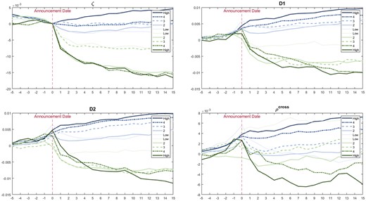
We also sort the stocks by , D1, D2, and to 10 deciles and plot the incremental probability of jumps, , before and after earnings announcements averaged over decile stocks in Figure 5.
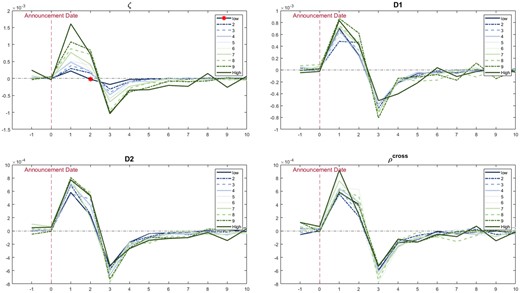
Changes in probability of jumps around earnings announcements.
Notes: These figures present the first difference in the jump’s probability, . We sort stocks into 10 deciles using different price efficiency measures. Then, we calculate changes in the jump’s probability averaged over decile stocks. We mark the point in the upper left figure with * to emphasize that it is negative and that jump’s probability starts to decline from the second day of earnings announcements.
The figure plots the changes in the jump’s probability before and after earnings announcements. Based on the results of the first decile stocks sorted by (dark blue line in the upper left figure), the jump intensity increases only slightly after the earnings announcement dates. More importantly, it starts to decline immediately after that. The figure displays distinct patterns of portfolio orders, while none of the other three measures can recover this pattern. However, the probability of jumps differs greatly from the PEAD. A substantial drift pattern following announcements does not necessarily indicate an increase in the probability of jumps. This may help to explain why D1 and D2 perform some tasks in sorting stocks with different CAR magnitudes but fail to do so when dealing with jump probabilities.
One can collect different news stories and compare |CAR| across assets after each type of news release. This can directly measure the incorporation speed of one specific type of news, but it requires prior information on news timeliness. Thus, we emphasize the convenience and generality of adopting as a measurement of stock price efficiency. Only asset returns must be known, and the timeliness of news is unnecessary. The model will determine whether jumps are present in the returns and whether they show clustering.
3.5 Jump’s Intensity Surrounding News Releases
As a supplementary illustration, we also investigate the dynamics of the jump’s intensity around news releases.
It has been well-established in the literature that stock price jumps are primarily driven by new information at both the macro level (Lee 2012) and the firm-specific level (Savor 2012; Bradley et al. 2014). However, there are very few formal investigations into when return jumps exhibit self/cross-excitation. Some literature provides possible directions on this topic. For example, the market may over- and under-react to the new information (Savor 2012; Jiang and Zhu 2017); stocks can vary depending on how quickly news is incorporated (Da, Gurun, and Warachka 2014; Tao, Brooks, and Bell 2021). Stocks with low pricing efficiency are predictable in the short run (Chordia, Roll, and Subrahmanyam 2008). These studies offer possible explanations for the clustering of more than two return jumps. It is not surprising to see another jump in a short period of time if the initial jump does not fully absorb the new information because of the market’s under-reaction or low pricing efficiency.
The model-estimated underlying intensity becomes a good object to examine the jump clustering and information arrivals. Note that is estimated to be equal to during the peaceful time. When a jump arriving at time t, will be raised by the jump. If another jump is observed before decays back to will become even higher; these two jumps form a cluster. Therefore, we can investigate ’s dynamics surrounding news announcements. Assuming a news announcement with a return jump occurs on date t, we should see an increase in the intensity at t + 1, which will then begin to decline over the next few days. However, if a jump clustering exists due to the low incorporation speed of news or under/over-reactions to the news, and a new jump is generated, we will see another increase in the intensity after t + 1.
| Macro-level | Federal Open Market Committee (FOMC) news releases |
| Nonfarm payroll employment report releases | |
| Unemployment rate releases | |
| Firm-specific | Earnings announcements |
| Dividend declarations |
| Macro-level | Federal Open Market Committee (FOMC) news releases |
| Nonfarm payroll employment report releases | |
| Unemployment rate releases | |
| Firm-specific | Earnings announcements |
| Dividend declarations |
| Macro-level | Federal Open Market Committee (FOMC) news releases |
| Nonfarm payroll employment report releases | |
| Unemployment rate releases | |
| Firm-specific | Earnings announcements |
| Dividend declarations |
| Macro-level | Federal Open Market Committee (FOMC) news releases |
| Nonfarm payroll employment report releases | |
| Unemployment rate releases | |
| Firm-specific | Earnings announcements |
| Dividend declarations |
Instead of reporting the long table of regression results, we plot the coefficient estimates in Figure 6. The full regression results are provided in Appendix A.4. We also provide some complementary results regarding this regression exercise in the Supplementary Appendix. The coefficient estimates for the macro-level and firm-specific news announcements are plotted on the left and right sides of Figure 6.

Coefficient estimates of regression on news announcements.
Notes: These two figures show the coefficient estimates of the regression Equation (19). We mark the coefficient estimates with * when they are significantly different from zero under a 5% significance level. The full regression results are provided in the Supplementary Appendix.
One must remember that under our model setting, an intensity increase at time t is caused by the jump that occurred at time t−1. However, looking at the left-side figure, the intensity increases on all three macro-announcement dates (), suggesting that there are jumps one day before the announcement. Regarding the earnings announcements, the first increase in intensity is the day after the announcements (), which shows evidence of jumps immediately after the earnings announcements. These results are consistent with three streams of literature: (1) jumps are closely related to the information releases (Lee 2012; Bajgrowicz, Scaillet, and Treccani 2016); (2) the information leakage of macro-news leads to pre-announcement drifts (Bernile, Hu, and Tang 2016; Kurov et al. 2019); (3) there are PEAD across assets (Bernard and Thomas 1989; Hung, Li, and Wang 2015). However, we are the first to aggregate these effects and explain them in terms of the probability of return jumps and their self-excitation.
Note that two subsequent increases in jumps’ intensities are evidence of their self-excitation. For example, the intensity increases on the day after the earnings announcements (), indicating the existence of jumps on the announcement dates (). It increases to a higher level on day two (), suggesting subsequent jumps on day one (), which create self-excitation of jumps and jump clustering. In other words, if a return series exhibits jumps at some specific dates but does not show jump clustering, the underlying intensity would not increase twice. Instead, it would increase once due to the first jump and then begin to decline. This can be caused by the fast information-incorporation speed of this information, which does not require a second jump to absorb the information.
We also remark that the coefficients on the earnings announcements are around 10 times greater than those on macro-announcements. This suggests that earnings announcements are when most jump clusterings occur (rather than during the releases of macro information).
4. Forecasting Performance
Another goal of this article is to examine whether jump clustering behaviors translate to the predictability of jumps and returns. We employ the forecasting framework outlined in Section 2.2 and conduct the out-of-sample forecasting. To facilitate the presentation of forecasting results, we continue to sort all US stocks by estimated in the in-sample period and form 10 portfolios to evaluate their out-of-sample performance.
4.1 RPS
The first out-of-sample exercise involves forecasting jumps’ probability (i.e., underlying intensity). We compare the RPS (see Equation (9) for the its calculation) from our forecasting methods with two benchmarks denoted as and . assumes jumps arrive independently. We re-estimate the model with constant jump intensities and . In , we let and . In , we assume there are no jumps in the price process. Thus, . To enable a fair comparison, we adopt a non-parametric jump filtering method to estimate as a proxy of jumps’ true values (see details in Appendix A.3). We also apply a Diebold-Mariano (DM) Test8 (Diebold and Mariano 2002) to determine whether the RPS from our model is superior to others.
Table 4 reports the RPS of 10 deciles of -sorted portfolios. The percentage in the table represents the proportion of stocks in each decile with RPSs lower than those of the benchmark. The value in brackets indicates the percentage of the portfolio’s stocks with p-values less than 0.05 in the Diebold–Mariano (DM) test. For example, the entry in the last row’s third column, 38.4% (18.9%) indicates that 38.4% of stocks in the decile present smaller RPSs, indicating superior forecasts against . Moreover, 18.9% of stocks are identified as having significantly lower RPS according to DM tests.
RPS of -sorted stock portfolios against two benchmarks
| No | |||||
|---|---|---|---|---|---|
| 1 | 0.021 | 20.2% (5%) | 1.4% (0%) | 1.8% (0%) | 0% (0%) |
| 2 | 0.028 | 22.7% (7.1%) | 2.1% (0%) | 2.8% (0%) | 0% (0%) |
| 3 | 0.033 | 26.2% (8.2%) | 4.6% (1.1%) | 3.9% (1.2%) | 0.8% (0.8%) |
| 4 | 0.037 | 25.9% (7.4%) | 2.8% (0.7%) | 2.5% (0.3%) | 0.8% (0.8%) |
| 5 | 0.041 | 20.9% (7.4%) | 3.5% (2.1%) | 3.2% (1.4%) | 3.1% (3.1%) |
| 6 | 0.047 | 21.3% (5.7%) | 6.4% (3.5%) | 4.6% (2.1%) | 5.8% (5.8%) |
| 7 | 0.054 | 25.5% (9.6%) | 10.3% (7.8%) | 5% (3.7%) | 17.9% (17.5%) |
| 8 | 0.065 | 25.9% (9.9%) | 17.4% (13.8%) | 10.5% (9.8%) | 23% (23%) |
| 9 | 0.083 | 37.6% (15.2%) | 18.8% (14.2%) | 16.1% (13.1%) | 31.9% (30.7%) |
| 10 | 0.139 | 34.2% (14.6%) | 28% (21.3%) | 25.2% (18.8%) | 34.6% (30.4%) |
Notes: This table presents the proportion of stocks in the decile with smaller-than-benchmark RPSs. The value in the bracket presents the percentage of the portfolio’s stocks having p-values less than 0.05 in the DM test. is the benchmark that assumes jumps arrive independently with constant jump intensities . In (). assumes there are no jumps in the price process ().
The tenth decile reporting the best performance, which is not surprising given its strongest jump clustering behaviors. We also recognize that the choice of true jump’s proxy and non-parametric jump filtering techniques may affect the outcomes. Additionally, it is less economically meaningful if one can only predict the probability of return jumps. Therefore, we would not extend the length of the article by reporting on extra results using alternative proxies and filtering methods. Instead, we focus on a more realistic evaluation of the forecasting framework—return predictions.
4.2 and Return Predictions
We estimate the and in the in-sample, and retrieve the empirical distribution . In the out-of-sample, we forecast underlying intensities and iteratively and collect returns when enters tails of the empirical distribution . The rules are defined in Equations (11) and (12). We plot ’s histograms of select well-known stocks in Figure 7. We also mark the 2.5th and 97.5th percentiles with red dash lines.
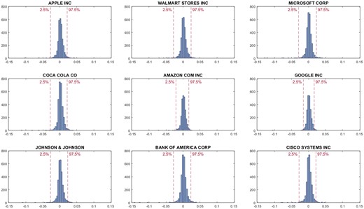
Histograms.
Notes: These figures show the empirical distribution of λ t d. The data period used in the estimation is from 1 January 2000 to 31 December 2012. The 2.5th and 97.5th percentiles are marked with red dash lines.
We run the regression for each individual asset, and the results are summarized in Table 5. Instead of presenting all the coefficient estimates, we summarize the F-statistics testing on all coefficients that are equal to 0. We also summarize the percentage of corresponding p-values that are smaller than 5% in the decile and the in the last two columns, where N is the total number of observations. Essentially, the is counting the percentage of returns whose is predicted to enter the tails of ’s empirical distribution. The F-stat indicates an increasing trend with the rise of . The decile also has more significant F-tests with higher .
F-statistics results summary
| No | F-stat | % of p-value 5% | % | |
|---|---|---|---|---|
| 1 | 0.0208 | 1.20 | 11.0 | 0.35 |
| 2 | 0.0280 | 2.65 | 24.8 | 0.74 |
| 3 | 0.0327 | 1.82 | 30.4 | 1.14 |
| 4 | 0.0369 | 2.26 | 41.8 | 1.20 |
| 5 | 0.0414 | 3.22 | 52.5 | 1.40 |
| 6 | 0.0470 | 3.17 | 53.5 | 1.76 |
| 7 | 0.0545 | 3.18 | 48.6 | 2.27 |
| 8 | 0.0653 | 4.59 | 48.9 | 3.88 |
| 9 | 0.0831 | 3.92 | 61.8 | 2.95 |
| 10 | 0.1388 | 5.42 | 73.6 | 5.81 |
Notes: We run the regression Equation (20) for each stock individually and collect the regression’s F-statistics testing on all coefficients being equal to 0. Then, we sort stocks by and calculate the average F-statistics of stocks in each decile. The fourth column presents the percentage of the F-test’s p-values that are smaller than 5% in the decile. The last column presents the average percentage of that equal 1 out of the total number of observations.
We also perform a regression on F-statistics with and some other measures. Table 6 presents the regression results. The results show that the degree of jump clustering does transfer to the out-of-sample predictive power and that stocks with higher are more predictable by our forecasting framework.
F-statistics cross-sectional regression
| F-stat | F-stat | F-stat | |
|---|---|---|---|
| 6.297*** | 5.497*** | 6.634*** | |
| (3.55) | (3.04) | (3.81) | |
| −7.273*** | −4.305 | ||
| (−2.89) | (−1.54) | ||
| D2 | 5.138*** | 2.5 | |
| (2.61) | (1.44) | ||
| D1 | −0.525 | −0.662 | |
| (−0.85) | (−0.99) | ||
| −1.777*** | |||
| (−3.54) | |||
| ivol | −0.478*** | ||
| (−3.57) | |||
| mkt cap | −0.048 | ||
| (−0.39) | |||
| b/m | 0.506** | ||
| (2.2) | |||
| illiquidity | 10.187 | ||
| (1.25) | |||
| Constant | 3.426*** | 3.159*** | 5.869*** |
| (12.68) | (7.45) | (6.22) | |
| 0.3% | 0.8% | 2.4% |
Notes: We run the regression Equation (20) for each stock individually and collect the regression’s F-statistics testing on all coefficients being equal to 0. Then, we run a regression on the F-statistics with a set of firms’ characteristics calculated in the in-sample period. ***, **, and * indicate statistical significance at the 1%, 5%, and 10% levels, respectively.
4.3 Trading on Jump Clustering
Another more straightforward way to assess the forecasting framework is by developing a trading strategy. The and can naturally serve as long and short trading signals, respectively. Specifically, we take a long position in the asset when the probability of positive jumps is predicted to be higher, and take a short position when the probability of negative jumps is predicted to be higher. Similarly, we report the performance of the -sorted portfolio. The results are reported in Table 7.
Performance of the trading strategy
| Buy-and-Hold | Trading Strategy | ||||||
|---|---|---|---|---|---|---|---|
| No | (%) | (%) | SR | (%) | (%) | SR | |
| 1 | 0.0208 | 15.2 | 22.5 | 0.67 | 28.1 | 63.2 | 0.44 |
| 2 | 0.0280 | 17.6 | 20.9 | 0.84 | 84.1 | 81.6 | 1.03 |
| 3 | 0.0327 | 18.4 | 19.9 | 0.92 | 140.7 | 176.7 | 0.80 |
| 4 | 0.0369 | 18.9 | 19.1 | 0.99 | 64.0 | 72.0 | 0.89 |
| 5 | 0.0414 | 18.6 | 19.7 | 0.94 | 95.1 | 76.8 | 1.24 |
| 6 | 0.0470 | 18.9 | 18.2 | 1.04 | 77.0 | 58.6 | 1.31 |
| 7 | 0.0545 | 17.4 | 19.3 | 0.90 | 121.4 | 87.9 | 1.38 |
| 8 | 0.0653 | 18.3 | 18.3 | 1.00 | 105.8 | 61.0 | 1.74 |
| 9 | 0.0831 | 19.9 | 18.3 | 1.09 | 145.0 | 86.3 | 1.68 |
| 10 | 0.1388 | 21.0 | 18.4 | 1.14 | 115.2 | 44.3 | 2.60 |
Notes: This table presents the equal-weighted returns, standard deviations and SRs of the trading strategy and corresponding buy-and-hold strategies. We sort all stocks by to 10 decile portfolios and report their performance separately.
In addition to the trading strategy, we also report the result of a buy-and-hold portfolio in the same decile for comparison. We calculate each strategy’s SR using its average excess return divided by its standard deviation (), where r denotes the risk-free rate. We use the US 10-year treasury note rate as a proxy of the risk-free rate. We also plot their cumulative log returns in Figure 8. Stocks with higher report better performance, and the SR of the stock’s portfolio can reach as high as 2.60.
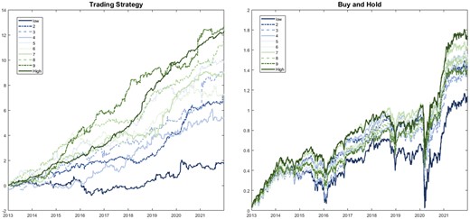
Cumulative log returns of the trading strategy and buy-and-hold strategy.
Notes: These two figures plot cumulative returns of the trading strategy and a buy-and-hold strategy across 10 portfolios. Stocks are categorized into these 10 portfolios by ζ.
4.3.1 Transaction costs
where and present the bid/ask price and the bid–ask spread, respectively, of stock s at time t. We only include half of the bid–ask spread in the transaction cost since the price data we used are the average of the bid and ask price. The results with transaction costs are presented in Table 8. The associated cumulative log returns are plotted in Figure 9. The trading strategy’s performance deteriorates since our forecasting framework is based on daily data. This means that the portfolio requires daily rebalancing. However, the portfolio with the highest still has an SR of 1.62.
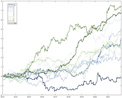
Cumulative log returns of the trading strategy with transaction costs.
Notes: This figure plots cumulative returns of the trading strategy with transaction costs across 10 portfolios. Stocks are categorized into these 10 portfolios by ζ.
Performance of the trading strategy with costs
| No | (%) | (%) | SR | |
|---|---|---|---|---|
| 1 | 0.0208 | 17.1 | 63.2 | 0.27 |
| 2 | 0.0280 | 57.0 | 81.5 | 0.70 |
| 3 | 0.0327 | 116.7 | 176.6 | 0.66 |
| 4 | 0.0369 | 44.3 | 71.8 | 0.62 |
| 5 | 0.0414 | 63.4 | 76.8 | 0.83 |
| 6 | 0.0470 | 58.3 | 58.4 | 1.00 |
| 7 | 0.0545 | 99.2 | 87.5 | 1.13 |
| 8 | 0.0653 | 67.6 | 60.7 | 1.11 |
| 9 | 0.0831 | 116.2 | 86.3 | 1.35 |
| 10 | 0.1388 | 84.8 | 52.3 | 1.62 |
Notes: This table presents the 10 stock portfolios’ equal-weighted returns, standard deviations and SRs of the trading strategy with transaction costs, including a fixed commission fee and liquidity costs represented by the bid–ask spreads.
Jump’s probability regressions on news releases
| Coef. () | t-stat | p-value | Coef. () | t-stat | p-value | ||
|---|---|---|---|---|---|---|---|
| 0.0336 | 1.68 | 0.09 | 0.0308 | 1.55 | 0.12 | ||
| 0.0665 | 3.00 | 0.00 | −0.0053 | −0.24 | 0.81 | ||
| 0.0753 | 2.93 | 0.00 | 0.3180 | 2.8 | 0.01 | ||
| 0.0351 | 2.28 | 0.02 | 0.9957 | 10 | 0.00 | ||
| −0.0188 | −1.35 | 0.18 | 0.1600 | 2.4 | 0.02 | ||
| 0.0051 | 0.26 | 0.80 | 0.0134 | 1.29 | 0.20 | ||
| 0.0179 | 0.81 | 0.42 | 0.0188 | 1.41 | 0.16 | ||
| 0.0392 | 1.67 | 0.10 | −0.0038 | −0.25 | 0.81 | ||
| 0.0229 | 0.80 | 0.42 | 0.0283 | 1.54 | 0.12 | ||
| −0.0210 | −1.17 | 0.24 | −0.0592 | −2.31 | 0.02 | ||
| 0.0323 | 1.18 | 0.24 | |||||
| 0.0505 | 2.28 | 0.02 | |||||
| 0.0815 | 3.2 | 0.00 | |||||
| 0.6530 | 2.59 | 0.01 | |||||
| −0.0114 | −1.22 | 0.22 | |||||
| Intercept | 0.0443 | 2057 | 0.00 | ||||
| Controls | Yes | ||||||
| Firm-fixed | Yes | ||||||
| Time-fixed | No | ||||||
| # Obs. | 8,399,706 | ||||||
| 1.49% |
Notes: This table presents the full regression results for Equation (19) and Figure 6. The control variables include log market cap, book-to-market ratio, illiquidity ratio, and idiosyncratic volatility.
5. Concluding Remarks
This study investigates the clustering behavior of return jumps across different assets modeled as a self/cross-exciting process embedded in a stochastic volatility model. We estimate the model using a Bayesian MCMC method. The contribution of this article is twofold. First, we introduce a novel measure of stock price efficiency, derived from the extent of jump clustering that an asset exhibits. We illustrate the superiority of this measure in capturing the cross-sectional variations in CAR following earnings announcements, which is robust to other existing measures and control variables.
Secondly, we assess the predictability of jumps based on the jump’s self/cross-exciting characteristics. We employ a particle filter to iteratively estimate latent variables in the out-of-sample and conduct one-step-ahead probabilistic forecasting for jumps. Based on RPSs, our forecasts outperform two benchmarks. We also introduce a new statistic representing the difference between the predicted probability of positive and negative jumps. We demonstrate the predictive efficacy of this statistic on returns, with its predictability directly inherited from the extent of jump clustering exhibited by the asset. Furthermore, we outline a trading strategy based on this forecasting framework, which reports an SR of 2.60 without transaction costs and 1.62 when accounting for the transaction costs.
Our studies shed light on the implication of return jump clustering behaviors and their predictability. The measure we introduce serves as a valuable tool for researchers and market participants aiming to evaluate stock price efficiency over a period of time. The results of our predictability assessment offer insights for individuals seeking to leverage jump clustering features to forecast return jumps and asset returns.
Footnotes
Part of the work was completed when Jian Chen attended ICMA Centre, Henley Business School, University of Reading, as a PhD student. I am indebted to my supervisors, Michael P. Clements and Andrew Urquhart, for their guidance. I am also very grateful for the extensive comments and discussions with Linquan Chen at the University of Exeter Business School. I also thank the editor, the associate editor, two anonymous referees, Shuyuan Qi, and the participants at the 2022 IAAE Annual Conference and 2022 CFE Conference for their helpful comments. All errors are mine.
Also see studies on news incorporation speed by Da, Gurun, and Warachka (2014), Tao et al. (2021), and Jeon et al. (2022).
These estimates derive from the stochastic volatility with correlated jumps model proposed by Duffie et al. (2000). The data used in the estimation are from 2000 to 2012, which is in line with the in-sample period of this paper.
Note in the calculation of , we use the Markov property of the jump intensity process to derive from , i.e., instead of from all past jumps . This can significantly speed up the algorithm.
To enable a fair comparison of against its benchmarks, we apply a non-parametric estimation on . We will introduce details of the estimation and benchmarks in Section 4.1.
The matrix represents the posterior mean of , i.e., .
Note that the regression is for all stock data; however, we suppress the notation specific to individual stocks for simplicity. For example, should be , representing of stock s and ‘s’ is suppressed.
We regress the stock returns with Fama–French three factors. The stock market beta is the coefficient estimate of the market factor, and the idiosyncratic volatility is the standard deviation of the estimated regression residuals.
Denote two series of probability score ( and ) from two different models. We calculate Diebold–Mariano statistic as DM = , where and denotes the autocovariance of at lag k. n denotes the number of forecasts, and we take .
Supplemental Material
Supplemental material is available at Journal of Financial Econometrics online.
Appendix A
Appendix A.1: Bayesian MCMC Algorithm and Specifications of Priors
We adopt a Bayesian MCMC algorithm to obtain the joint posterior distribution in Equation (5). We randomly draw samples from conditional posterior distributions. Our sampling algorithm is as follows:
Bayesian MCMC Algorithm
For :
1: Sample k static parameters:
Draw from ,
Draw from
2: Sample jumps
for :
Draw from ,
Draw from ,
Draw from ,
3: Sample jump sizes
for :
Draw from ,
Draw from ,
Draw from ,
4: Sample variance:
for t = 1,2, …, T:
Draw from ,
We ran our MCMC algorithm for 100,000 iterations; the first 50,000 is considered a burn-in period. We sample the posterior distribution by a hybrid of Gibbs sampling and Metropolis-Hastings. Gibbs sampling methods are used when conjugate priors of conditional posteriors are available. We adopt the Metropolis–Hastings sampling method for others whose posteriors are not available in closed form. Details of posterior distributions are provided by Lazar and Qi (2022) and Rasmussen (2013). Our specifications of priors are as follow:
| Parameters | Prior distribution | Parameters | Prior distribution |
|---|---|---|---|
| N (0, 25) | |||
| N (50, 100) | IG (10, 40) | ||
| IG (10, 40) | |||
| IG (10, 20) | |||
| Parameters | Prior distribution | Parameters | Prior distribution |
|---|---|---|---|
| N (0, 25) | |||
| N (50, 100) | IG (10, 40) | ||
| IG (10, 40) | |||
| IG (10, 20) | |||
| Parameters | Prior distribution | Parameters | Prior distribution |
|---|---|---|---|
| N (0, 25) | |||
| N (50, 100) | IG (10, 40) | ||
| IG (10, 40) | |||
| IG (10, 20) | |||
| Parameters | Prior distribution | Parameters | Prior distribution |
|---|---|---|---|
| N (0, 25) | |||
| N (50, 100) | IG (10, 40) | ||
| IG (10, 40) | |||
| IG (10, 20) | |||
Appendix A.2: Particle Filter
We adopt a particle filter to sample latent variables in the out-of-sample period. The particle filtering method is given by Pitt and Shephard (1999). Creal (2012) also gives a review of this technique. Our ultimate goal is to sample from to obtain estimates of latent variables at each time t, where . We remark that we ignore sampling jump sizes since they are less relevant to forward simulating jump intensities . We adopt a sequential importance sampling with a re-sampling scheme:
Sequential Importance Sampling with Re-sampling
At t = 0, for
Draw , set
For :
1: For , draw .
2: Compute importance weights .
3: Normalize importance weights .
4: Re-sample N particles by and reset .
See more details of particle filtering in Creal (2012), where codes of the particle filtering algorithm are also available.
Appendix A.3: Non-Parametric Jump Filtering
Appendix A.4: Full Regression Results of Figure 6
This table presents the full regression results for Equation (19) and Figure 6. We collect data for five types of news release dates. Then, we perform regressions using five dummy variables for each type of news representing from 1 day before the news release to 5 days after the news release. The data used in the regression are US stock data from 2000 to 2012. Note we did not impose a time-fixed effect since it is correlated with the macro-news release dates (Table A.4).
