


Abstract
Estimating parameters of amino acid substitution models is a crucial task in bioinformatics. The maximum likelihood (ML) approach has been proposed to estimate amino acid substitution models from large datasets. The quality of newly estimated models is normally assessed by comparing with the existing models in building ML trees. Two important questions remained are the correlation of the estimated models with the true models and the required size of the training datasets to estimate reliable models. In this article, we performed a simulation study to answer these two questions based on simulated data. We simulated genome datasets with different numbers of genes/alignments based on predefined models (called true models) and predefined trees (called true trees). The simulated datasets were used to estimate amino acid substitution model using the ML estimation methods. Our experiments showed that models estimated by the ML methods from simulated datasets with more than 100 genes have high correlations with the true models. The estimated models performed well in building ML trees in comparison with the true models. The results suggest that amino acid substitution models estimated by the ML methods from large genome datasets are a reliable tool for analyzing amino acid sequences.

Introduction
The amino acid (AA) substitution model describes the substitution rates among 20 AAs during the evolution. The substitutions among AAs are typically modelled by a time-continuous, time-homogeneous Markov process. The model is continuous in time indicating that the AA substitutions can happen at any point during the evolution process. The time-homogeneous property assumes that the substitution rates among AAs remain constant throughout the entire process. The AA substitution process is irreducible; therefore, it has a stationary distribution, i.e., the frequencies of AAs during the evolution are at equilibrium. The core component of the Markov process is the transition rate matrix Q representing the number of substitutions from one AA to another AA per time unit. The transition rates can be inferred from the exchangeability rates (i.e., the rate of change) between AAs and their frequencies. The AA substitution process might be assumed to be time-reversible indicating that the exchangeability rates between two AAs are the same in both directions. This assumption reduces the computational effort in estimating and using the models, however, the time-reversible property might be not biologically realistic and does not allow us to reconstruct rooted trees.
The AA substitution models play a vital role in analyzing the evolutionary relationships among protein sequences. They are used to calculate the likelihood values of phylogenetic trees to determine the maximum likelihood (ML) tree. They can be also employed as the score matrices to determine the similarity between protein sequences in sequence similarity searches or multiple sequence alignment algorithms.
The nucleotide substitution model has a small number of parameters that can be directly estimated from the alignment under the study. The AA substitution model contains a much larger number of parameters, i.e., 189 parameters for time-reversible models or 379 parameters for time-nonreversible models. A single-protein alignment does not provide enough information to estimate the parameters of the AA model. The parameters of the AA substitution model can be better estimated by using more data (Müller et al., 2002). Therefore, a big dataset of protein alignments is required to estimate the parameters of the AA substitution model to overcome the overfitting problem when estimating a large number of parameters (Dang et al., 2022; Le & Gascuel, 2008; Minh et al., 2021; Vinh, 2021; Whelan & Goldman, 2001).
A number of models have been empirically estimated from general datasets containing a large number of protein alignments of various species such as WAG (Whelan & Goldman, 2001) or LG (Le & Gascuel, 2008). Several clade-specific models have been estimated for different clades such as Q.mammal, Q.insect, Q.bird, Q.yeast, or Q.plant for mammals, insects, birds, yeasts, and plants, respectively (Minh et al., 2021). The empirically estimated models are called fixed models as their parameters are fixed.
In ML analyses, the best-fitting model for a specific alignment is normally selected from a set of available fixed models. However, it is possible that none of the available fixed models is appropriate for the alignment under the study. A number of methods have been proposed to enhance the use of fixed AA substitution models in Bayesian inferences such as average inferences over a set of fixed models (Huelsenbeck et al., 2008).
Several ML methods have been proposed to estimate AA substitution models (Dang et al., 2014, 2022; Le & Gascuel, 2008; Minh et al., 2021; Whelan & Goldman, 2001). The ML method QMaker has been introduced to estimate the time-reversible models from whole genome datasets (Minh et al., 2021). The authors applied QMaker to estimate several time-reversible models from genomes of plants, birds, yeasts, mammals, and insects. The clade-specific models outperform the existing models in building ML trees for their corresponding data.
The time-reversible assumption is mathematically and computationally convenient, however, studies revealed that the assumption may be violated (Naser-Khdour et al., 2019; Squartini & Arndt, 2008). Recently, the nQMaker method has been proposed to estimate time-nonreversible models from genome datasets (Dang et al., 2022). Experiments show that the time-nonreversible models are likely better than the time-reversible models in analyzing large alignments. Crucially, the time-nonreversible models allow us to reconstruct rooted phylogenetic trees.
To date, the quality of a newly estimated model is normally assessed by comparing it with existing models in building ML trees. For a real training dataset, the true AA substitution model is unknown, therefore, we are unable to evaluate the correlation between the estimated model and the true model; or compare the performance of the estimated model and the true model in building ML trees. The required size of a training dataset to estimate a reliable model is an important open question.
In this article, we used the alignment simulation program AliSim (Ly-Trong et al., 2022) to simulate different datasets each containing N alignments/genes generated from four predefined AA substitution models (i.e., Q.plant, NQ.plant, Q.bird, and NQ.bird) and two predefined phylogenetic trees (i.e., the plant tree (Ran et al., 2018) and the bird tree (Jarvis et al., 2015)). The predefined model and the predefined tree used to generate a simulated dataset are considered/called the true model and the true tree of the simulated dataset. For each simulated dataset, we used the QMaker and nQMaker programs (Dang et al., 2022; Minh et al., 2021) to estimate a time-reversible model and a time-nonreversible model, respectively. We performed a number of analyses to directly compare the estimated models with the true models. We also assessed the ability of the estimated models in building ML trees in comparison with the true models.
Materials and methods
Data
We used the AliSim program (Ly-Trong et al., 2022) to simulate AA alignments. The AliSim program requires five parameters to simulate an alignment: a predefined AA substitution model, a site rate heterogeneous model, a phylogenetic tree, and the number of sequences together with the sequence length of the alignment. We simulated alignments with both time-reversible AA substitution models (called time-reversible alignments) and time-nonreversible AA substitution models (called time-nonreversible alignments).
We used real parameters obtained from the plant genome dataset of 1,000 genes, each containing 35 sequences (Ran et al., 2018) and the bird genome dataset of 6,295 genes, each consisting of 48 sequences (Jarvis et al., 2015) to simulate plant and bird genome datasets.
- Simulating plant genome datasets: To create a simulated dataset of N alignments/genes , we randomly selected N genes from the plant genome. For each selected gene, the sequence length, the time-reversible substitution model Q.plant, the site rate heterogeneity model (estimated from the selected gene), and the unrooted phylogenetic tree (Minh et al., 2021) were provided to simulate a time-reversible alignment. Similarly, we used the time-nonreversible substitution model NQ.plant and the rooted phylogenetic tree (Dang et al., 2022) to simulate a time-nonreversible alignment.
- Simulating bird genome datasets: We used the same above procedure to simulate bird genome datasets with different numbers of alignments .
For each simulation condition (a combination of plant or bird with the number of alignments N), we produced five simulated datasets. Each simulated dataset was used to estimate one AA substitution model. These models are called simulated models. Thus, we obtained five simulated models for each simulation condition.
To compare the performance of simulated models and the true models in building ML trees, we used the testing datasets including 308 plant testing genes and a subset of 500 bird testing genes obtained from the QMaker’s paper (Minh et al., 2021).
Methods
Estimating parameters of amino acid substitution model
We assume that the evolutionary process is independent among AA sites. We use a Markov process to model the AA substitution process with time-homogeneous, time-continuous, and stationary assumptions. The core component of the model is the so-called matrix of 20 × 20 instantaneous substitution rates among AAs. Technically, represents the number of substitutions from AA to AA per time unit. We assign the diagonal values such that the sum of all elements on row of equals zero. In phylogenetic analyses, the branch length of phylogenetic trees indicates the number of AA substitutions per site, therefore, we normalize so that the total number of substitutions is one. Technically, is divided by the normalization factor , where is the equilibrium frequency of AA . The normalized matrix has 379 parameters.
To reduce the computational burdens, we might assume that the AA substitution process is time-reversible (i.e., the exchangeability rates between AA and AA are equal in both directions). As a result, the matrix can be decomposed into two parts: a symmetric exchangeability rate matrix and an AA frequency vector such that . The R matrix contains 189 parameters and the vector consists of 19 parameters.
A training dataset used to estimate an AA substitution model includes N alignments denoted by . Let be the set of N trees for the training alignments, i.e., is the tree of alignment . As AA substitution rates vary among sites, the best site rate model is selected for each alignment. Typically, a site rate model combines a distribution of rates, a proportion of invariant sites (Gu et al., 1995; Yang, 1993), or a distribution-free rate model (Yang, 1995). Let } be the set of site rate models for the training alignments, i.e., is the site rate model for alignment .
The ML estimation method determines the parameters of model Q, the phylogenetic trees T, and the parameters of site rate models P to maximize the likelihood value . We can calculate the likelihood value over N alignments of D as following:
Optimizing with a large number of parameters is a computationally expensive task. Fortunately, the previous studies show that the parameters of Q can be optimized based on nearly optimal trees T and site rate models P (Dang et al., 2014, 2022; Le & Gascuel, 2008; Minh et al., 2021). Thus, the parameters of Q, T, and P can be estimated iteratively instead of simultaneously to overcome the computational burdens. In this article, we used the recently published ML estimation methods QMaker and nQMaker (Dang et al., 2022; Minh et al., 2021) to estimate time-reversible models and time-nonreversible models from the simulated datasets, respectively.
Alignment simulation
We used the AliSim program (Ly-Trong et al., 2022) to simulate alignments based on parameters of real alignments. Given a real alignment , the procedure to simulate an alignment includes two steps (see Figure 1) described as follows:
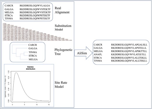
The procedure to simulate an alignment using parameters from a real alignment, a predefined amino acid substitution model, a predefined phylogenetic tree, and a site rate heterogeneity model.
- Parameter inference step: Consider a real alignment including sequences with sequence length . If is selected from plant (bird) genome dataset, set the predefined AA substitution model Qdefined by the Q.plant (Q.bird) model, and the predefined tree Tdefined by the plant (bird) tree. We used the IQ-TREE2 program (Minh et al., 2020) to determine the best site-rate heterogeneity model for .
- Simulation step: The model Qdefined, the tree Tdefined, and the site-rate model were subsequently used to simulate the alignment with sequences of length using the AliSim program.
To generate a dataset D of N alignments, we conducted the simulation procedure N times with N different real alignments.
Model analyses and comparison
Let Qsim be the AA substitution model estimated from a simulated dataset. The model Qsim is called a simulated model. More precisely, let QsimN be the AA substitution model estimated from a simulated dataset of N alignments, e.g., Qsim100 be the AA substitution model estimated from a simulated dataset of 100 alignments.
First, we calculated the Pearson correlation between the true substitution model and the estimated model. We also analyzed the difference between AA substitution rates of the true model and that of the simulated model.
Second, we compared the quality of the simulated model Qsim and the true model Qdefined in building ML trees on testing alignments. For each testing alignment if the ML tree constructed with the true model Qdefined is better (worse) than the tree constructed with the simulated model Qsim, the true model Qdefined is considered better (worse) than the simulated model Qsim.
Third, we measured the similarity between trees constructed with the true models and those constructed with the simulated models using the Robinson–Foulds (RF) distance (Robinson & Foulds, 1981). The RF distance is the number of splits which exist in one tree but not in the other tree. The RF distance is normalized by dividing by the total number of splits. The normalized RF distance (nRF) ranges from 0 (i.e., two trees are identical) to 1 (i.e., two trees are completely different).
Results
Model analysis
For each simulation condition, the average correlation between the true model and five simulated models was analyzed. First, we compared the true models Q.plant with simulated models Qsim.plant; and the true model NQ.plant with simulated models NQsim.plant with respect to different numbers of genes (see Figure 2). The simulated models Qsim.plant and NQsim.plant estimated from ≥ 100 genes have high correlations with the true models. For example, the average correlation between the true model Q.plant and simulated models Qsim100.plant is 0.997. The average correlation between the true model NQ.plant and simulated models NQsim100.plant is close to 1. We note that the correlations between the true models and simulated models estimated from 200 or 250 alignments are all close to 1.
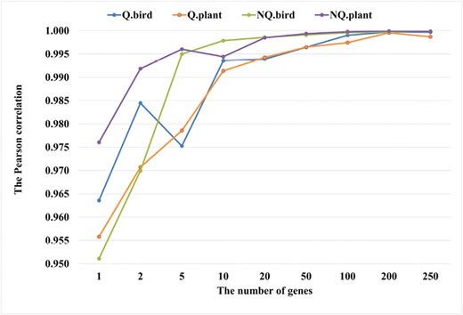
The average Pearson correlations between the true model and simulated models for different simulation conditions. The simulated models estimated from datasets with ≥ 100 genes are highly correlated with the true models.
We observed similar results for the bird datasets. The simulated model Qsim.bird estimated with ≥ 100 genes has high correlations with the true model Q.bird (i.e., 0.999 for 100 genes; 0.9997 for 200 genes, and 0.9999 for 250 genes). The correlations between simulated models and the true models get higher with the increase in training data size used to estimate the models. For example, the average correlations between the true model NQ.bird and the simulated models NQsim.bird with 10, 100, and 200 genes are 0.9954, 0.9995, and 0.9997, respectively.
We calculated the standard deviation of correlations between the true model and the simulated models for every simulation condition (see Table 1). All standard deviations are small and close to 0 for the simulation conditions with ≥ 100 genes.
The standard deviation of correlations between the true models and simulated models for different simulation conditions.
| #genes Models | 1 | 2 | 5 | 10 | 20 | 50 | 100 | 200 | 250 |
|---|---|---|---|---|---|---|---|---|---|
| Q.plant | 0.0110 | 0.0136 | 0.0043 | 0.0032 | 0.0032 | 0.0009 | 0.0011 | 0.0009 | 0.0006 |
| NQ.plant | 0.0048 | 0.0082 | 0.0007 | 0.0016 | 0.0004 | 0.0001 | 0.0001 | 0.0001 | 0.0001 |
| Q.bird | 0.0291 | 0.0105 | 0.0063 | 0.0060 | 0.0024 | 0.0014 | 0.0006 | 0.0003 | 0.0002 |
| NQ.bird | 0.0143 | 0.0147 | 0.0023 | 0.0020 | 0.0007 | 0.0002 | 0.0001 | 0.0001 | 0.0001 |
Calculating the Pearson correlation coefficient is a simple way to measure the linear correlation between two matrices. However, we note that the Pearson correlation depends on the range of substitution rates of the matrices. It is sensitive to large substitution rates, i.e., large substitution rates have a high impact on the value of Pearson correlation between two matrices.
For more details, we directly analyzed the relative differences between substitution rates of the matrices. We counted the number of substitution rates in the simulated models that are at least 2 times or 5 times larger (smaller) than that in the true models. Table 2 shows the comparisons between the true model Q.plant and its highest correlation model Qsim.plant for the plant datasets; and between the true model Q.bird and its highest correlation model Qsim.bird for the bird datasets. For example, 29 out of 400 elements in the simulated model Qsim100.plant are at least 2 times greater than that in the true model Q.plant; and 9 elements are at least 2 times smaller than that in Q.plant. The simulated models estimated from datasets with less than 100 genes contain a considerable number of substitution rates that are at least 2 times different from that in the true models. There are only few elements in the simulated models estimated from 200 or 250 genes that are 2 times or 5 times different from that in the true models. Figure 3 demonstrates the relative difference between the true model Q.plant and its highest correlation model Qsim100.plant (Figure 3A), and between the true model Q.bird and its highest correlation model Qsim100.bird (Figure 3B).
The average number of substitution rates that 2 times larger (2×), 5 times larger (5×), 2 times smaller (−2×), and 5 times smaller (−5×) when comparing time reversible model Q.plant and simulated model Qsim.plant; and between Q.bird and simulated model Qsim.bird.
| Number of genes | ||||||||||
|---|---|---|---|---|---|---|---|---|---|---|
| Comparing models | Larger/Smaller | 1 | 2 | 5 | 10 | 20 | 50 | 100 | 200 | 250 |
| Qsim.plant vs. Q.plant | 2× | 171.8 | 154.6 | 108.6 | 85.2 | 56.6 | 38.8 | 29.8 | 18.6 | 13.2 |
| 5× | 150 | 126 | 80.4 | 59.6 | 34.4 | 19.8 | 13 | 8.4 | 6.8 | |
| −2× | 48 | 48 | 32 | 33 | 18.8 | 11.4 | 9.8 | 8.8 | 6.4 | |
| −5× | 17.6 | 14.2 | 9.8 | 8.8 | 4.4 | 4.6 | 4.4 | 4.2 | 4 | |
| Qsim.bird vs. Q.bird | 2× | 218.8 | 148.2 | 136.6 | 93.6 | 69.6 | 38.8 | 36.2 | 18.4 | 14.4 |
| 5× | 199 | 132.8 | 109.4 | 71.6 | 34.4 | 12.4 | 8 | 3.6 | 2 | |
| −2× | 39.4 | 49 | 34.6 | 27.2 | 12.8 | 5.8 | 0.6 | 1.8 | 1.2 | |
| −5× | 12.6 | 9.6 | 5.6 | 3.6 | 0.4 | 0.4 | 0 | 0.4 | 0 | |
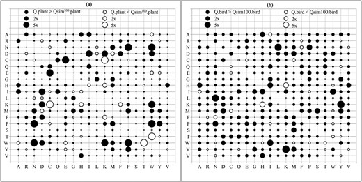
The bubble plots show relative differences between amino acid substitution rates in Q.plant and its highest correlation model Qsim100.plant (A); and between Q.bird and its highest correlation model Qsim100.bird (B). Both Qsim100.plant and Qsim100.bird were estimated from 100 genes. Notations: 2 × (5×) indicates that the substitution rate between two models is at least 2 times (5 times) different.
Figure 4 displays the distribution of mean squared errors (MSE) between substitution rates of the true model and those of the simulated models (the MSE were calculated from five simulations). The highest MSE are 0.443 for the bird matrices and 0.329 for the plant matrices. For the case of 100 genes, the highest MSE of and are 0.052 and 0.172, respectively. The average of all MSE of is 0.00076 for the bird matrices and 0.00056 for the plant matrices.
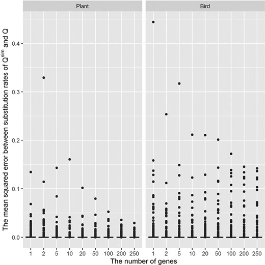
The distribution of mean squared errors between substitution rates of the true model Q.plant and simulated models Qsim.plant (left); and the true model Q.bird and simulated models Qsim.bird (right). The mean squared errors were calculated from five simulations.
Similarly, we compared the time-nonreversible models NQsim.plant and NQsim.bird with their corresponding true models NQ.plant and NQ.bird (see Table 3). For example, the NQsim100.plant model consists of 39 substitution rates that are at least 2 times different from that in the true model NQ.plant. Similarly, the NQsim100.bird model contains 30 substitution rates that are at least 2 times different from that in the true model NQ.bird. As the time-nonreversible models consist of more parameters than the time-reversible models, more training data are required to estimate time-nonreversible models so that they are close to the true models. Figure 5 demonstrates the relative difference between the true model NQ.plant and its highest correlation model NQsim100.plant (Figure 5A); and between the true model NQ.bird and its highest correlation model NQsim100.bird (Figure 5B).
The average number of amino acid substitution rates that 2 times larger (2×), 5 times larger (5×), 2 times smaller (−2×), and 5 times smaller (−5×) when comparing the true model NQ.plant with simulated model NQsim.plant; and between NQ.bird with simulated model NQsim.bird.
| Number of genes | ||||||||||
|---|---|---|---|---|---|---|---|---|---|---|
| Comparing models | Larger/Smaller | 1 | 2 | 5 | 10 | 20 | 50 | 100 | 200 | 250 |
| NQsim.plant vs. NQ.plant | 2× | 210 | 178.6 | 126 | 106.8 | 74.8 | 49.6 | 39.2 | 25 | 18.8 |
| 5× | 196.2 | 164.8 | 110.2 | 88.2 | 60.2 | 37.2 | 25.4 | 18.8 | 14 | |
| −2× | 51.4 | 54.4 | 52.4 | 49.4 | 43 | 28.4 | 23.2 | 17.6 | 17.2 | |
| −5× | 22.6 | 22.6 | 14 | 12.6 | 12.2 | 9.6 | 4 | 4 | 3.6 | |
| NQsim.bird vs. NQ.bird | 2× | 244.2 | 182.4 | 146.8 | 106 | 81.6 | 48.2 | 30.6 | 15 | 15.6 |
| 5× | 236.2 | 171 | 134.4 | 92.4 | 61.6 | 28.4 | 15.4 | 7 | 8.2 | |
| −2× | 41.8 | 53.6 | 57.6 | 56.8 | 41 | 18.6 | 11.2 | 7.2 | 7.6 | |
| −5× | 19.6 | 18.8 | 16.2 | 13.6 | 5.6 | 2 | 2 | 1.8 | 1.2 | |
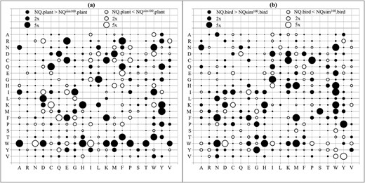
The bubble plots show relative differences between amino acid substitution rates in NQ.plant and its highest correlation model NQsim100.plant (A); and between NQ.bird and its highest correlation model NQsim100.bird (B). Both NQsim100.plant and NQsim100.bird were estimated from 100 genes. Notations: 2 × (5×) indicates that the substitution rate between two models is at least 2 times (5 times) different.
Figure 6 shows the distribution of MSE between substitution rates of nonreversible models (the MSE were calculated from five simulations). The MSE of the time-nonreversible matrices are lower than that of the time-reversible matrices. They are all smaller than 0.205 and close to zero when the number of genes ≥ 100.
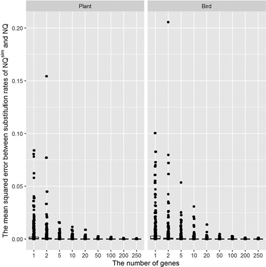
The distribution of mean squared errors between substitution rates of the true model NQ.plant and simulated models NQsim.plant (left); and the true model NQ.bird and simulated models NQsim.bird (right). The mean squared errors were calculated from five simulations.
Likelihood comparison
We used log-likelihood values to examine the performance of simulated models in building ML trees (see Figure 7). We compared the average log-likelihood values of 5 simulated models with that of the true model for each simulation condition. We note that a simulated model is considered better (worse) than the true model for a testing alignment if the tree constructed with the simulated model has a higher (lower) log-likelihood value than that constructed with the true model.
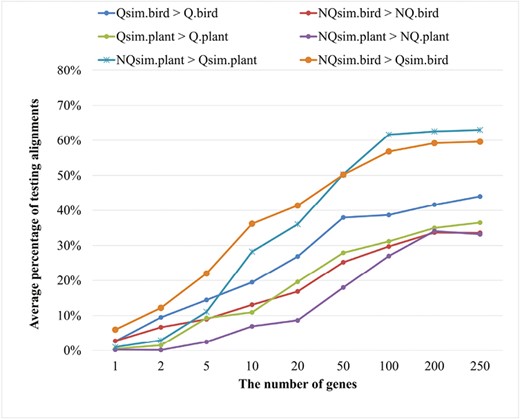
The performance of the true models and the simulated models in building ML trees for different simulation conditions. The average proportion of testing alignments where the simulated model yields better a log-likelihood value than the true model.
Figure 7 shows that trees constructed with true models have higher likelihood values than those constructed with simulated models for a large number of testing alignments. The likelihood of trees with simulated models gets closer to that with the true models when more genes are used to estimate models. For example, trees constructed with Q.plant have higher likelihood values than those with Qsim10.plant, Qsim50.plant, and Qsim100.plant for 89.9%, 72.1%, and 68.8% of testing alignments, respectively.
We also examined the performance of reversible models Qsim and nonreversible models NQsim in building ML trees (see Figure 7). The nonreversible models NQsim estimated from small datasets (i.e., less than 50 genes) were not as good as their corresponding reversible models Qsim. The performance of NQsim gets better with the increase in training data size used to estimate the models. For example, NQ100sim.plant was better than Q100sim.plant in building ML trees for 61.69% of the plant alignments; and NQ100sim.bird was better than Q100sim.bird for 56.8% of the bird alignments. It is recommended to use model selection programs such as ModelFinder (Kalyaanamoorthy et al., 2017) to determine the best-fit model for the alignment under study (Dang et al., 2022; Minh et al., 2021).
The simulated plant models estimated from ≥ 100 genes performed considerably well in building ML trees in comparison with the true models. For example, the simulated model Qsim100.plant helped build better ML trees than the true model Q.plant in 31.1% of testing alignments. Similarly, the simulated model NQsim100.plant outperformed the true model NQ.plant in building ML trees for about 27% of testing alignments.
We obtained similar results for the bird datasets. The simulated models Qsim100.bird and NQsim100.bird were better than the true models Q.bird and NQ.bird in 38.6% and 31.4% of the testing alignments, respectively. The simulated bird models estimated from small datasets including 10 or 20 genes were worse than the true models for a majority of testing cases.
Topology comparison
We examined the topological difference between trees constructed with the true models and those with the simulated models. The average nRF distances (see Table 4) show that trees constructed with the true models and those with the simulated models are mostly identical. For plant alignments, trees inferred using the simulated models estimated from ≥ 20 genes are identical to trees constructed with the true model. For the bird alignments, the average nRF distances between trees constructed with the true models and those inferred using the simulated models estimated from ≥ 100 alignments are close to zero. For reversible models, the average nRF distances between trees constructed with simulated models and those inferred with the true models are zero when ≥ 50 genes were used to estimate the models (the average nRF distances between trees built with the general model LG and those with the true models are 0.006 and 0.022 for the plant and bird datasets, respectively). Table 4 shows that the nRF distances between true trees and trees inferred from individual genes are small for the plant dataset, and considerably large for the bird dataset.
The average nRF distances among the plant tree, the bird tree, and trees constructed with the simulated models and the true models. If , two trees have identical topology.
| #genes nRF | 1 | 2 | 5 | 10 | 20 | 50 | 100 | 200 | 250 |
|---|---|---|---|---|---|---|---|---|---|
| Q.plant vs. Qsim.plant | 0 | 0.012 | 0.006 | 0 | 0 | 0 | 0 | 0 | 0 |
| NQ.plant vs. NQsim.plant | 0.018 | 0.012 | 0.012 | 0.006 | 0 | 0 | 0 | 0 | 0 |
| Q.bird vs. Qsim.bird | 0.020 | 0 | 0.106 | 0.004 | 0.004 | 0 | 0 | 0 | 0 |
| NQ.bird vs. NQsim.bird | 0.120 | 0.04 | 0.238 | 0.048 | 0.088 | 0 | 0.035 | 0.09 | 0.039 |
| Qsim.plant vs. plant tree | 0.031 | 0.018 | 0.025 | 0.031 | 0.031 | 0.031 | 0.031 | 0.031 | 0.031 |
| NQsim.plant vs. plant tree | 0.018 | 0.018 | 0.025 | 0.031 | 0.031 | 0.031 | 0.031 | 0.031 | 0.031 |
| Qsim.bird vs. bird tree | 0.556 | 0.529 | 0.556 | 0.556 | 0.556 | 0.556 | 0.556 | 0.556 | 0.556 |
| NQsim.bird vs. bird tree | 0.507 | 0.511 | 0.409 | 0.538 | 0.528 | 0.538 | 0.542 | 0.451 | 0.416 |
We also analyzed the average branch length of trees reconstructed with the simulated models for different simulation conditions (see Table 5). The average branch length of the true plant tree is 0.051. The average branch length of plant trees constructed with the simulated models ranges from 0.0061 to 0.065. For example, the average branch lengths of trees constructed with Qsim100.plant and NQsim100.plant are 0.062 and 0.061, respectively. The true bird tree has an average branch length of 0.017. The bird trees built with the simulated models have average branch lengths from 0.027 to 0.032. The average branch lengths of trees constructed with Qsim100.bird and NQsim100.bird are both equal to 0.027. In general, the bigger training datasets resulted in better models for estimating the branch lengths of trees. Note that the simulated models estimated from ≥ 100 genes produced trees with similar branch lengths.
The average of branch length of trees constructed with the simulated models for different simulation conditions.
| #genes | 1 | 2 | 5 | 10 | 20 | 50 | 100 | 200 | 250 |
|---|---|---|---|---|---|---|---|---|---|
| Qsim.plant | 0.065 | 0.064 | 0.063 | 0.062 | 0.062 | 0.062 | 0.062 | 0.062 | 0.062 |
| NQsim.plant | 0.064 | 0.063 | 0.062 | 0.061 | 0.061 | 0.061 | 0.061 | 0.061 | 0.061 |
| Qsim.bird | 0.030 | 0.028 | 0.028 | 0.027 | 0.027 | 0.027 | 0.027 | 0.027 | 0.027 |
| NQsim.bird | 0.032 | 0.029 | 0.027 | 0.027 | 0.027 | 0.027 | 0.027 | 0.026 | 0.027 |
We also calculated the MSE and standard deviations of branch lengths of trees constructed with the simulated models in comparison with the true trees (see Table 6). The MSE values are small and decrease with the increase in the number of genes. For example, the average MSE values of trees with Qsim1.plant is 0.001003 and that with Qsim100.plant is 0.000848.
The average of mean square errors (×1,000) and standard deviations (×1,000) of the average branch length of trees inferred with the simulated models in comparison with the plant tree and the bird tree.
| #genes | Qsim.plant | Qsim.bird | NQsim.plant | NQsim.bird | ||||
|---|---|---|---|---|---|---|---|---|
| MSE | SD | MSE | SD | MSE | SD | MSE | SD | |
| 1 | 1.003 | 0.120 | 2.218 | 0.310 | 1.033 | 0.124 | 2.044 | 0.542 |
| 2 | 0.974 | 0.133 | 1.989 | 0.167 | 0.877 | 0.056 | 1.913 | 0.338 |
| 5 | 0.893 | 0.032 | 2.219 | 0.312 | 0.827 | 0.036 | 1.836 | 0.357 |
| 10 | 0.845 | 0.009 | 1.901 | 0.130 | 0.811 | 0.012 | 1.789 | 0.115 |
| 20 | 0.856 | 0.018 | 1.773 | 0.103 | 0.806 | 0.004 | 1.916 | 0.568 |
| 50 | 0.851 | 0.014 | 1.774 | 0.130 | 0.795 | 0.005 | 1.727 | 0.053 |
| 100 | 0.848 | 0.009 | 1.844 | 0.114 | 0.795 | 0.004 | 1.840 | 0.135 |
| 200 | 0.853 | 0.005 | 1.775 | 0.133 | 0.795 | 0.004 | 1.945 | 0.234 |
| 250 | 0.848 | 0.003 | 1.735 | 0.106 | 0.793 | 0.004 | 1.829 | 0.209 |
Discussion
The ML methods have been proposed to estimate both time-reversible and time-nonreversible models from genome datasets. The true AA substitution models are unknown for real data; therefore, we are unable to evaluate the quality of estimated models in comparison with the true models based on real data. In this article, we compared the estimated models and the true models based on the simulated data. Our study based on the simulated genome datasets with different numbers of genes revealed that both time-reversible and time-nonreversible models estimated by the ML methods from large genome datasets (i.e., datasets with 100 or more genes) are highly correlated with the true model.
The estimated models from large datasets performed well in building ML phylogenetic trees. The significant tests showed that the models derived from large genome datasets and the true models were not significantly better than each other for a majority of testing alignments. The tree topologies constructed with the simulated models and that inferred with the true models are nearly identical. As the true models are not available, the models estimated from large datasets can be reliably used in studying the evolution of protein sequences.
Estimating AA substitution models from large genome datasets is very time-consuming. Only five simulations per set were performed in this study because it took us months to estimate all models from both QMaker and nQMaker estimation methods with different simulation conditions. We note that the standard deviations of all estimated models with ≥ 100 genes and the true models are close to zero.
Data availability
The datasets and scripts used in this article are available at https://doi.org/10.6084/m9.figshare.22336384.
Author contributions
Nguyen Huy Tinh (Investigation [equal], Software [equal], Visualization [equal], Writing—original draft [equal]), Cuong Dang (Conceptualization [equal], Methodology [equal], Resources [lead], Supervision [equal], Writing—review & editing [supporting]), and Vinh Le (Conceptualization [equal], Funding acquisition [lead], Methodology [equal], Project administration [lead], Supervision [equal], Writing—review & editing [lead])
Funding
This research was funded by the Vietnam National Foundation for Science and Technology Development (NAFOSTED; [102.01.2019.06 to C.C.D. and L.S.V.]).
Conflicts of interest
All authors declare that they have no conflict of interest.
