


Abstract
Colour is an important component of many different defensive strategies, but signal efficacy and detectability will also depend on the size of the coloured structures, and how pattern size interacts with the background. Consequently, size‐dependent changes in colouration are common among many different species as juveniles and adults frequently use colour for different purposes in different environmental contexts. A widespread strategy in many species is switching from crypsis to conspicuous aposematic signalling as increasing body size can reduce the efficacy of camouflage, while other antipredator defences may strengthen. Curiously, despite being chemically defended, the gold‐striped frog (Lithodytes lineatus, Leptodactylidae) appears to do the opposite, with bright yellow stripes found in smaller individuals, whereas larger frogs exhibit dull brown stripes. Here, we investigated whether size‐dependent differences in colour support distinct defensive strategies. We first used visual modelling of potential predators to assess how colour contrast varied among frogs of different sizes. We found that contrast peaked in mid‐sized individuals while the largest individuals had the least contrasting patterns. We then used two detection experiments with human participants to evaluate how colour and body size affected overall detectability. These experiments revealed that larger body sizes were easier to detect, but that the colours of smaller frogs were more detectable than those of larger frogs. Taken together our data support the hypothesis that the primary defensive strategy changes from conspicuous aposematism to camouflage with increasing size, implying size‐dependent differences in the efficacy of defensive colouration. We discuss our data in relation to theories of size‐dependent aposematism and evaluate the evidence for and against a possible size‐dependent mimicry complex with sympatric poison frogs (Dendrobatidae).
Abstract

INTRODUCTION
Aposematic (warning) colouration signals directly to potential predators that prey is not profitable and is best avoided (Caro & Ruxton, 2019; Mappes et al., 2005; Stevens & Ruxton, 2012). Once predators learn or evolve to associate particular colours and patterns with negative experiences, aposematic species are then freed from the constraints of camouflage and better able to utilize their environments with a reduced risk of costly predator encounters (Arbuckle et al., 2013; Speed et al., 2010).
Aposematic signals are frequently characterized by bright colours and high‐contrast patterns, which are distinct from palatable prey species, and that can be easily recognized and learnt by potential predators (Mappes et al., 2005; Stevens & Ruxton, 2012). Bright longwave colours, such as red and yellow, combined with black patterning are commonly associated with warning signals, as these colours create high chromatic and achromatic contrast across the body and are distinct from many natural substrates (Aronsson & Gamberale‐Stille, 2009, 2012; Gamberale‐Stille, 2001; Prudic et al., 2006; Stevens & Ruxton, 2012). Aposematic signals are, however, best conceptualized along a spectrum from camouflaged to conspicuous that trades off the costs and benefits of detectability and saliency depending on factors including defence strength, behaviour, habitat use and the composition of the predator community (Barnett et al., 2016a, 2016b; Blount et al., 2009; Endler & Mappes, 2004; Higginson & Ruxton, 2010; Mappes et al., 2005; Postema et al., 2022).
The gold‐striped frog, Lithodytes lineatus (Leptodactylidae), is predominantly black with a pair of bright yellow dorsolateral stripes and red femoral spots. The dorsolateral stripes are always visible, but the femoral spots can be hidden and displayed facultatively as a presumed deimatic signal (Cintra et al., 2014; Prates et al., 2012; Umbers et al., 2017). These frogs are chemically defended and so aposematism is likely to be the primary driver of colour evolution (Prates et al., 2012), although skin secretions may also be involved in chemical crypsis within the nests of leaf‐cutter ants where these frogs are commonly found (de Lima Barros et al., 2016). Frogs of different sizes do, however, seem to differ in the colour of the dorsolateral stripes which appear to be less bright and more cryptic in larger individuals. Such differences suggest the precise balance between salient signalling and camouflage is associated to some extent with frog size (Lamar & Wild, 1995; Regös & Schlüter, 1984).
Aposematic signals are generally considered to become more effective with increasing body size as colouring becomes more salient and prey secondary defences strengthen (Forsman & Merilaita, 1999; Hagman & Forsman, 2003; Stevens & Ruxton, 2012). In contrast, camouflage is thought to become less effective at larger body sizes as the area of apparent pattern mismatch will increase (Pembury Smith & Ruxton, 2021; Remmel & Tammaru, 2009; Xiao, 2015). As such, many species will change from being cryptic as juveniles to being brightly coloured adults (Booth, 1990). For example, certain lepidopteran caterpillars, including Saucrobotys futilalis (Crambidae), switch from cryptic to aposematic colouring as they grow larger and can no longer easily hide among the vegetation (Grant, 2007).
Relative body size can, however, also influence predation risk in other ways as detectability and the value predators ascribe to prey may differ according to prey size (Barnett et al., 2011; Flores et al., 2015; Halpin et al., 2013; Higginson & Ruxton, 2010; Remmel & Tammaru, 2009, 2011; Smith et al., 2014, 2016). For instance, if toxin concentrations do not increase at the same rate as body mass, predators may favour larger prey as the costs of toxin ingestion decrease relative to the benefits of greater nutritional gain (Barnett et al., 2007, 2011; Smith et al., 2014, 2016). Similarly, ontogenetic changes in behaviour and habitat use can change the balance between salient signalling and camouflage, with camouflage being less effective for more active and diurnal life stages (Hall et al., 2013; Higginson & Ruxton, 2010; Ioannou & Krause, 2009; Merilaita & Tullberg, 2005; Speed et al., 2010; Stevens & Ruxton, 2019; Valkonen et al., 2014; Yin et al., 2015). In several grasshoppers (Romaleidae), for example, a switch from a gregarious juvenile stage to a solitary adult is accompanied by a switch from conspicuous warning signals to camouflage (Despland, 2020), and in the eastern newt (Notophthalmus viridescens (Salamandridae)) the aposematic, terrestrial, juvenile ‘eft’ will transform into a cryptically coloured, aquatic, adult (Brodie, 1968).
In addition to potential aposematism, the yellow horseshoe pattern found in L. lineatus is reminiscent of a common colour form seen in the putative aposematic signals of several species of toxic poison frog (Dendrobatidae), for example: Ameerega picta, Dendrobates truncatus and Phyllobates aurotaenia. Consequently, it has long been suspected that L. lineatus may be a mimic of poison frogs (Nelson & Miller, 1971; Rojas, 2017). Many early reports assumed L. lineatus to be a Batesian mimic (Lamar & Wild, 1995; Regös & Schlüter, 1984), but now that toxic skin secretions have been identified, L. lineatus is largely considered a potential Müllerian mimic (Prates et al., 2012). It has consequently been hypothesized that colour variation in L. lineatus may be the result of size‐dependent mimicry, where colour contrast is maximized when body size overlaps with that of sympatric poison frogs and is reduced at larger sizes where the benefits of mimicry decrease (Lamar & Wild, 1995, Regös & Schlüter, 1984).
In masquerade, the mimicry of uninteresting rather than dangerous objects, appropriate body size is important for effective camouflage and ontogenetic changes in colour often occur when body size exceeds that of the mimicked structure (Postema, 2022; Skelhorn, Rowland, & Ruxton, 2010; Skelhorn, Rowland, Speed, et al., 2010; Skelhorn & Ruxton, 2012). A comparable shift from Batesian mimicry to camouflage has been reported for the microhylid frog Oreophyryne ezra (Microhylidae) and the bushveld lizard Heliobolus lugubris (Lacertidae), both of which are apparent mimics of noxious beetles as juveniles before becoming cryptic as adults (Bulbert et al., 2017; Huey & Pianka, 1977). Conversely, as defended co‐mimics can both educate potential predators, size‐dependent mimicry may be expected to have a weaker influence on Müllerian mimicry systems (Pfennig & Mullen, 2010). Importantly, however, despite its widespread adoption, empirical evidence for or against mimicry in L. lineatus is currently lacking.
Here, we examined how differences in colour and body size affect the detectability of L. lineatus to evaluate whether multiple defensive strategies, including aposematism, mimicry and camouflage, may be at play for differently sized frogs. We expected that if conspicuous signalling is only favoured for smaller individuals, the dorsolateral stripes, which are always visible, would be less detectable in larger frogs. However, as the femoral spots are hidden and are unlikely to attract the attention of predators, we expected high‐contrast colours would be retained regardless of body size. We first used visual modelling to assess how colour contrast differed depending on frog size, and then ran two detection experiments with human participants to evaluate how both colour and body size affected detectability. We then discuss these data in relation to possible scenarios for the evolution of aposematism and/or mimicry, to review the evidence for and against widespread assumptions regarding the mimicry hypothesis, and to highlight avenues for future research.
MATERIALS AND METHODS
Photography
In May–July 2019, we captured and photographed a series of differently sized L. lineatus (n = 30, 18–59 mm SVL) and photographed patches (~500 × 700 mm) of their natural leaf litter background (n = 504) at the Iyarina Forest Reserve, Provincia de Napo, Ecuador (Figure 1) (Anderson et al., 2021). We searched for frogs among the leaf litter along diurnal and nocturnal transects through an area of mature secondary forest and the surrounding disturbed scrub and grassland. We took the leaf litter background photographs at ~2–5 m intervals along nonlinear transects through the forest avoiding patches occluded by plant growth. All photographs were taken under natural diffuse daylight illumination with a Nikon D7200 DSLR camera and AF‐S DX NIKKOR 35 mm lens (Nikon Corp. Japan), were saved in RAW format, and each contained a ColorChecker Passport (X‐Rite Inc., USA) that allowed us to colour calibrate (400–700 nm) and scale the images (Stevens et al., 2007; Troscianko & Stevens, 2015).
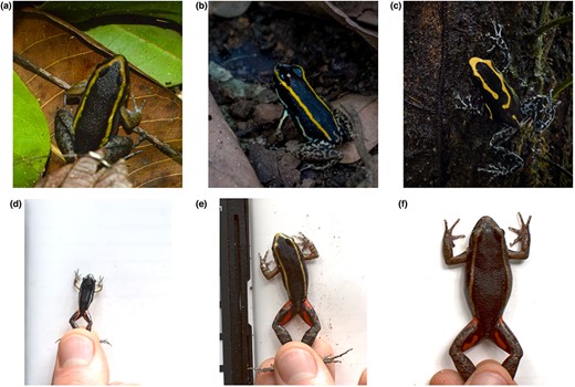
Study system. Top. Examples of convergent evolution in conspicuous colouration between Lithodytes lineatus (Leptodactylidae) and two poison frogs (Dendrobatidae), Phyllobates lugubris (allopatric) and Dendrobates tinctorius (sympatric): (a) = L. lineatus, (b) = P. lugubris, and (c) = D. tinctorius. Bottom. Size dependent colouring found in Lithodytes lineatus: (d) = small (19 mm), (e) = medium (38 mm) and (f) = large (58 mm). Photo credits: (a) = Martin Hinojosa, (b & c) = James B. Barnett and (d–f) = all authors.
Spectrophotometry
To check whether our photography methods captured all visually relevant wavelengths, we measured reflectance values from a mid‐sized (39 mm SVL) L. lineatus and from four colours of fallen leaves (n = 10 per colour), with an Ocean Optics Flame S‐XR1‐ES (200–1025 nm) spectrophotometer and DH‐Mini Deuterium Tungsten Halogen (200–2500 nm) light source (Ocean Optics Inc. USA). We took three measurements from each leaf, and for the frog, we took three measurements from the dorsum and four each from the stripes and spots. Each measurement was the average of three 5 s scans, taken with the probe held at a 45° angle, 3 mm away from the sample. Mean spectra (300–700 nm) were calculated, smoothed, and plotted in R package pavo in R v.4.0.5 (Maia et al., 2019; R Core Team, 2021). As neither the frog nor leaf litter significantly reflected UV wavelengths (300–400 nm) we used the photographs to model visual contrast (Figure 2 left).
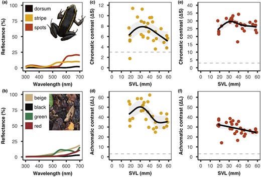
Visual modelling. Left: Spectrophotometry reflectance curves (300–700 nm) from (a) the dorsum, stripe and spots of a mid‐sized (39 mm) Lithodytes lineatus and (b) four colour classes of forest floor leaves (inset squares show exaggerated colours to differentiate plotted lines). There was minimal UV reflectance (300–400 nm) from the frog and from the leaf litter background. Middle and right: Internal pattern contrast represented as (c) chromatic and (d) achromatic contrast between the dorsum and the stripe, and (e) chromatic and (f) achromatic contrast between the dorsum and the spots. The solid black lines represent the estimated GAM smoothing curves, the grey shading represents 95% confidence intervals, and the horizontal dashed line represents the visual discrimination threshold (3 JND). There was no significant effect of body size on chromatic contrast, however, achromatic contrast changed with body size. The achromatic contrast of the stripes peaked in mid‐sized individuals, whereas the achromatic contrast of the spots decreased with increasing body size.
Calculating visual contrast
We used the MICA Toolbox in ImageJ v.1.52 k to calculate visual contrast (Schneider et al., 2012; Troscianko & Stevens, 2015). We created a custom camera calibration profile and modelled the tetrachromatic vision of the Indian peafowl (Pavo cristatus, Phasianidae), which in the absence of UV reflectance is similar to many different species of predatory bird (Ödeen & Håstad, 2003). The peafowl has single cone peak sensitivities (λmax) of L = 605, M = 537, S = 477, V = 432, and double cones with λmax of 567 nm (Hart, 2002). We set Weber fractions to 0.05, calculated chromatic contrast (ΔS = hue) from the responses of the L, M and S single cones, and achromatic contrast (ΔL = luminance) from the response of the double cone. We selected regions of interest (ROIs) from each of the 30 frogs, corresponding to two or three representative patches of the dorsal, stripe and spot colours. For each frog, we then calculated ΔS and ΔL between the dorsum and both the stripe and spot colours (Darst et al., 2006; Yeager & Barnett, 2020, 2021).
Visual inspection of our data showed that the relationship between visual contrast and body size was likely to be nonlinear. We, therefore, used generalized additive models (GAMs) with thin plate regression splines from R package mgcv (Wood, 2011) to analyse these relationships in R v.4.0.5 (R Core Team, 2021). GAMs allow for a flexible approach in identifying both linear and nonlinear relationships without making any prior assumptions about the functional form of the interaction. These models use multiple basis functions that are summed to create a nonparametric smoothing function (hereafter referred to as a “smooth”). The selection of the smoothing term was done by the restricted maximum likelihood method (REML) which penalizes overfitting (Wood, 2011). In all cases, we used a Gaussian error distribution and identity link. We used the function gam.check in mgcv to assess model fit through diagnostics tests and visual inspection of the residual distributions (Wood, 2011).
We analysed ΔS and ΔL separately for both stripe and spot contrast, and we included frog size (SVL in mm) as the independent variable in each model. The significance of the smooth terms was assessed using F tests provided by the summary function for each GAM. A p value < 0.05 indicated that a flat horizontal line could not be fitted through the 95% CI of the smooth term. The effective degrees of freedom (edf) represent the number of basis functions fit to the relationship with a value of 1 representing a linear relationship and higher values indicating an increasingly complex relationship between visual contrast and body size.
Detection experiments
We randomly selected 100 background photographs and selected all the frogs from three size classes: <20 mm (n = 5), 30–40 mm (n = 11) and >50 mm (n = 6). Frog size and colour varied continuously (Figure 2c–f) and so categories were chosen to represent the lower extreme, middle and upper extreme of the size distribution. As linearized images appear dark, we exported each ROI with a 20% nonlinear transform from the MICA Toolbox (Troscianko & Stevens, 2015). As the dimensions of the background ROIs varied slightly, we standardized the aspect ratio of each background image by cropping the ROIs to the largest rectangle that would fit within all the background ROIs (~630 × 480 mm). We then used MATLAB 2021a (The MathWorks, Inc. USA) to make the frog stimuli. We first calculated the mean value of each RGB colour channel for each frog ROI (multiple samples from the dorsum, stripes and spots from each frog), next we calculated the mean of these RGB values for each colour region of each frog (creating a single value per frog for each ROI type), and then the mean across each frog size class (single value for the dorsum, stripe and spot colours for each size class).
We used a photograph of a mid‐sized (39 mm) L. lineatus in a natural resting posture to create a standardized template which was used in all subsequent detection experiments. To create the different treatments, we recoloured the template to make four colour conditions for each of the three age classes (n = 12 treatments). These age classes were: S = small frogs (<20 mm), M = medium frogs (30–40 mm), and L = large frogs (>50 mm). The unique colours of each size condition were combined into four pattern manipulations: A = dorsal colour only, B = dorsal and spot colours, C = dorsal and stripe colours, and D = dorsal, stripe and spot colours (Figure 3).
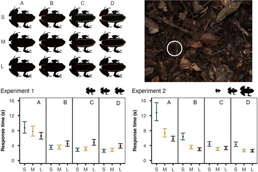
Detection experiments. Top‐left: The 12 colour treatments used in both experiments (S = small (<20 mm), M = medium (30–40 mm), L = large (>50 mm) | A = dorsal, B = dorsal and spot, C = dorsal and stripe, D = dorsal, stripe, and spot). Top‐right: An example of the experimental stimuli (treatment MD at 35 mm on the leaf litter background—highlighted by white circle). Bottom. Response time (seconds; means ±95% CI from the model) for each experiment (green = S, orange = M, black = L). Silhouettes indicate relative size between S, M, and L treatments. In experiment 1 (left) all treatments were presented at a standardized size (35 mm), and in experiment 2 (right) each size class was presented at its natural size (S = 20 mm, M = 35 mm and L = 50 mm).
In experiment 1, we examined how colour affected detectability while controlling for variation in body size. To do this we kept all stimuli at a standardized length equivalent to 35 mm relative to the background (Figure 3). In experiment 2, we were interested in the potential interaction between colour and size, and so frogs were scaled to maintain their true sizes (A = 20 mm, B = 35 mm, and C = 50 mm) relative to the background (Figure 3). It is important to note that in experiment 2, although body length increased by a set value (15 mm) between each size treatment (20, 35 and 50 mm), the area of the target increased by the square of the scale factor. The large treatments, therefore, had a length 2.50 times longer but an area 6.25 times larger than the small treatments.
We recruited 163 human participants through McMaster University's online subject coordination system (Sona Systems Ltd., Tallin, Estonia), and alternately assigned each to either experiment 1 (n = 75) or experiment 2 (n = 88). The difference in participant number between experiments is the result of some participants withdrawing from the study after having been assigned to a treatment group but before data were collected. Each participant was given written instructions and took part in the experiment online, on a personal computer and at a time chosen by themselves. For each participant, we presented 4 replicates of each of the 12 treatments (n = 48 stimuli per participant). Each frog stimulus was rotated by a number of degrees, between 1 and 360, selected at random from a uniform distribution. Each frog stimulus was then pasted onto a randomly selected background image at a location selected at random from a two‐dimensional uniform distribution while ensuring that the whole frog was visible on the screen. Background selection, frog rotation and frog placement were randomized independently for each participant such that all stimuli presentations were unique. Participants were tasked with locating and clicking on the frog as quickly and as accurately as possible with their mouse cursor. We recorded the time taken to click on the frog (response time = RT) for all frogs that were correctly identified. We then analysed log‐transformed response time for each experiment with a linear mixed effect model in R package lme4 in R v.4.0.5 (Bates et al., 2014; R Core Team, 2021). We included the main effects of treatment and conducted pairwise general linear hypothesis tests to compare between age classes (S v M, S v L and M v L) for each colour treatment (A, B, C and D). Pairwise tests were conducted using the glht function from R package multcomp and p values were corrected using the single‐step method (Hothorn et al., 2008).
RESULTS
Visual contrast
When analysing the contrast between the dorsum and the dorsal stripe, we found a general trend for peak contrast to be found with mid‐sized individuals. Specifically, the relationship between body size and chromatic contrast was seemingly nonlinear but marginally nonsignificant (F = 2.77, edf = 2.34, p = 0.093), whereas there was a significant, non‐linear, relationship between body size and achromatic contrast (F = 3.53, edf = 3.07, p = 0.020). Achromatic contrast increased between body sizes of ~18–32 mm, slowly decreased between ~32–49 mm and then plateaued between ~50–59 mm (Figure 2c,d).
When assessing visual contrast between the dorsum and the red femoral spots, we found a general inverse relationship where contrast decreased as body size increased. There was a marginally nonsignificant, seemingly nonlinear, change in chromatic contrast (F = 2.90, edf = 2.90, p = 0.096), but a significant, linear, relationship between body size and achromatic contrast (F = 5.74, edf = 1.00, p = 0.024), where ΔL decreased consistently from 18–59 mm (Figure 2e,f).
Detection: Experiment 1
In experiment 1, all frogs were presented at the same size relative to the background; the equivalent to a mid‐sized individual (35 mm). We found a significant effect of treatment on response time, and so we conducted pairwise comparisons between the age classes for each pattern manipulation (Table 1; Figure 3 bottom‐left). We found that dorsal colour was more detectable in larger frog size classes, with no difference in response time found between the S and M frogs (SA = MA) or the M and L frogs (MA = LA), but the dorsal colour of S frogs did take significantly longer to detect than that of L frogs (SA > LA). Conversely, when the dorsal colour was combined with either the stripe or spot colours, the colours of large frogs were detected more slowly than the colours of small or medium sized frogs. There was no difference in detection time between S and M frogs in the spot (SB = MB), stripe (SC = MC) or combined stripe and spot (SD = MD) conditions. However, detection time for S and M was significantly shorter than L in the spot (SB < LB | MB < LB), stripe (SC < LC | MC < LD) and combined (SD < LD | MD < LD) conditions.
Detection experiment results. In experiment 1 all frogs were presented scaled to a common size (35 mm) and in experiment 2 frogs were presented at their natural sizes (S = 20 mm, M = 35 mm, L = 50 mm) relative to the background.
| Experiment 1 | ||||
| Main effect of treatment: χ2 = 529.98, df = 11, p < 0.001 | ||||
| A | B | C | D | |
| S – M | z = 1.36, p = 0.836 | z = −0.18, p > 0.999 | z = −1.16, p = 0.926 | z = −1.22, p = 0.904 |
| S – L | z = 3.29, p = 0.011 | z = −3.47, p = 0.006 | z = −7.55, p < 0.001 | z = −5.96, p < 0.001 |
| M – L | z = 1.96, p = 0.407 | z = −3.28, p = 0.012 | z = −6.35, p < 0.001 | z = −4.75, p < 0.001 |
| Experiment 2 | ||||
| Main effect of treatment: χ2 = 689.53, df = 11, p < 0.001 | ||||
| A | B | C | D | |
| S – M | z = 5.96, p < 0.001 | z = 9.02, p < 0.001 | z = 5.48, p < 0.001 | z = 7.31, p < 0.001 |
| S – L | z = 8.50, p < 0.001 | z = 11.59, p < 0.001 | z = 4.38, p < 0.001 | z = 7.91, p < 0.001 |
| M – L | z = 2.83, p = 0.051 | z = 2.61, p = 0.095 | z = −1.05, p = 0.957 | z = 0.62, p = 0.999 |
Note: Treatment codes: Size class (S = small, M = medium, L = large) and colour manipulations (A = dorsal only, B = dorsal and spots, C = dorsal and stripe, D = dorsal, spot, and stripe). Results from fitted generalized linear mixed effects models, and pairwise general linear hypothesis tests. Pairwise comparisons where p < 0.05 are highlighted in bold.
Detection: Experiment 2
In experiment 2, each frog size class was presented at its true size (S = 20 mm, M = 35 mm, L = 50 mm) relative to the background. There was a significant effect of treatment on response time, and we conducted pairwise comparisons between size classes for each colour manipulation (Table 1; Figure 3 bottom‐right). We found that the dorsal colour of the frogs became easier to find with increasing size, with detection time being greater for S frogs than both M (SA > MA) and L (SA > LA), while the difference in detection time between M frogs and L frogs was marginally nonsignificant (MA = LA). Similarly, when spots, stripes or both were added to the dorsal colours, we found that frogs were easier to find at larger sizes. We found no difference in detection time between M and L frogs for the spot (MB = LB), stripe (MC = LC) and combined (MD = LD) treatments. However, detection time for S frogs was significantly longer than both M and L frogs in the spot (SB > LB | MB > LB), stripe (SC > LC | MC > LD), and combined (SD > LD | MD > LD) conditions.
DISCUSSION
Our data suggest that colour variation represents differences in the balance between antipredator defences according to body size, with smaller frogs displaying high contrast, highly detectable colours, whereas larger frogs exhibit colours more suited for camouflage. However, body size is also an important factor in detectability with larger frogs being more detectible than smaller frogs even when displaying more cryptic colours. Much of this colour variation was explained by varying brightness rather than hue, and we found size‐dependent differences in saliency in both the stripes and the spots. The achromatic contrast of the dorsolateral stripes peaked in mid‐sized individuals, whereas the contrast of the red femoral spots generally decreased with increasing body size. This colour variation corresponded to differences in detectability, such that when controlling for size, the colours of small‐ and medium‐sized frogs were more detectable than those of large frogs. However, when presenting frogs at their true relative sizes, the trend was reversed with medium and large frogs being found more quickly than small frogs.
A change from conspicuous to cryptic colouring suggests that the benefits of aposematic signalling only outweigh the benefits afforded by camouflage in smaller frogs. Larger body size makes detection easier, but the bright colours of mid‐sized individuals make mid‐sized frogs more detectable than would be expected from body size alone. Such a change may be explained by changes in morphology, behaviour and habitat use as frogs get larger (Booth, 1990; Higginson & Ruxton, 2010; Kikuchi et al., 2021). Juvenile L. lineatus are more diurnally active than larger individuals, and as such movement may reduce the efficacy of camouflage and expose juveniles to more visually guided predators (Lamar & Wild, 1995; Regös & Schlüter, 1984). Similarly, aposematism may be less effective for larger frogs. It is possible that toxin production may be intrinsically lower in larger L. lineatus, but in other chemically defended frogs, toxin reserves appear to increase with increasing body size (Jeckel et al., 2015; Saporito et al., 2012, 2010). However, as toxins are secreted by glands in the skin, even if toxin production remains high, larger size may result in a lower surface area to volume ratio and a correspondingly lower concentration of poison relative to body mass (Prates et al., 2012).
Moreover, there is sexual dimorphism in size with females being on average larger than males (Bernarde & Kokubum, 2009). Males conspicuously call to attract females (Lamar & Wild, 1995, Regös & Schlüter, 1984), and so camouflage may be less effective and aposematism a more successful defence for smaller conspicuous males, while females can better rely on camouflage. Indeed, the role of colour in intra‐ or intersexual communication, conflict or mate choice has yet to be tested empirically. We do not, however, find a clear bimodal colour distribution that would be expected if colour was primarily driven by sexual dimorphism and future work is needed to evaluate how males and females may differ in colour, behaviour and toxicity.
We also observed, contrary to our predictions, that this decrease in achromatic contrast and detectability occurred in both the dorsolateral stripes and the femoral spots. Changes in dorsolateral stripe colour may be explained by varying trade‐offs in optimal detection distance (Postema et al., 2022), but as the femoral spots remain hidden at rest, it is less clear why frogs of different sizes would differ in signal characteristics (Drinkwater et al., 2022). Indeed, it has been suggested that larger prey species are more likely to exhibit deimatic behaviours as camouflage is less effective (Drinkwater et al., 2022; Kang et al., 2017; Loeffler‐Henry et al., 2019; Pembury Smith & Ruxton, 2021). In this case, the larger size of the deimatic signal appears to counteract the decrease in achromatic contrast, at least in terms of initial detection time. It is, however, important to note that colour is just one component of deimatic defence (Drinkwater et al., 2022).
It has also long been suggested that L. lineatus may mimic the salient colours of poison frogs, however, more data are needed to effectively evaluate this hypothesis and several conceptual aspects must be clarified before conclusions can be drawn. Bright yellow dorsolateral stripes have evolved independently in many different species of poison frog, found both within and outside of the range of L. lineatus (Grant et al., 2006; Vences et al., 2003). We found that L. lineatus was most contrasting and most detectable at sizes (~18–40 mm) that roughly correspond to the range of body sizes recorded for the majority of these poison frog species (Grant et al., 2006). There may then appear to be some circumstantial evidence of a size‐dependent mimicry complex. Across its range, however, L. lineatus overlaps with many different, similarly coloured, but unrelated, species of poison frog, many of which only occur in relatively small, nonoverlapping, geographic regions (Cintra et al., 2014; Grant et al., 2006; Guillory et al., 2019). Furthermore, across large swathes of its range (including at our study site) there appear to be no chemically defended frogs of an appropriate size or colour to act as co‐mimics. In such cases, aposematism may act independently, or innate generalized avoidance and/or predator migration between areas may allow mimics to exist beyond the range of their models (Pfennig & Mullen, 2010). It is, however, currently unknown if and how mimicry may function across these large spatial scales and patchy distributions. Alternatively, apparent mimicry may be an artefact of hypotheses developed before chemical defences were identified in L. lineatus and conspicuous colours could seemingly not be attributed to aposematism. To better evaluate the mimicry hypothesis, therefore, we first need to know the context within which conspicuous colouring initially evolved, and then how subsequent range expansion may have brought different species into contact. Consequently, pre‐existing, convergent evolution may currently be the most parsimonious explanation for apparent similarities to poison frogs.
Taken together we found that size‐dependent differences in the colouration of L. lineatus shift the balance between conspicuous signalling and camouflage. This change suggests a strong selective advantage for conspicuous signalling in smaller individuals, but that the benefits of greater saliency decrease relative to the benefits of camouflage in the larger frogs. This effect on colour is pronounced despite larger body sizes being harder to camouflage effectively, but the factors underpinning this effect are still unclear. Size‐dependent mimicry remains a possibility, but further work is needed to understand whether natural predators which have learnt to avoid poison frogs will also avoid L. lineatus, whether the colours of L. lineatus provide a more effective signal within the natural range of potential co‐mimics, and whether there is any evidence of local adaptation where signal characteristics track the colours and body size of different co‐mimics in different locations.
AUTHOR CONTRIBUTIONS
James B. Barnett: Conceptualization (lead); data curation (lead); formal analysis (lead); investigation (equal); methodology (lead); project administration (lead); software (equal); validation (lead); visualization (lead); writing – original draft (lead); writing – review and editing (lead). Justin Yeager: Conceptualization (lead); funding acquisition (lead); investigation (lead); methodology (equal); project administration (lead); resources (lead); supervision (lead); writing – original draft (equal); writing – review and editing (equal). Brendan L. McEwen: Conceptualization (equal); data curation (equal); investigation (equal); methodology (equal); writing – original draft (supporting); writing – review and editing (supporting). Isaac Kinley: Conceptualization (supporting); data curation (equal); formal analysis (equal); investigation (equal); methodology (equal); software (lead); writing – original draft (supporting); writing – review and editing (supporting). Hannah M. Anderson: Conceptualization (equal); investigation (equal); methodology (equal); writing – original draft (supporting); writing – review and editing (supporting). Jennifer Guevara: Data curation (equal); formal analysis (lead); writing – original draft (supporting); writing – review and editing (supporting).
ACKNOWLEDGEMENTS
For their help in the field, we thank Raul Costa‐Pereira (Universidade Estadual de Campinas, Brazil), David N. Fisher (University of Aberdeen, UK), James L. L. Lichtenstein (Yale University, CT, USA) and Martin Hinojosa (Universidad Regional Amazónica Ikiam, Ecuador), and for advice on the statistical analyses we thank N. Simon Sanghera. We thank the Universidad de Las Américas for funding provided to Justin Yeager (Grant/Award Number: FGE.JY.20.13), and Jonathan N. Pruitt (McMaster University) for providing additional funding (NSERC Canada 150 Chair). We would also like to thank all the staff at the Andes and Amazon Field School (Ecuador) for their invaluable assistance in the field and access to field sites.
CONFLICT OF INTEREST
We declare we have no conflicts of interest.
PEER REVIEW
The peer review history for this article is available at https://publons.com/publon/10.1111/jeb.14143.
DATA AVAILABILITY STATEMENT
Raw data are available in the DRYAD digital repository, https://doi.org/10.5061/dryad.4xgxd25cf.
