


Abstract
Allometric scaling describes the relationship of trait size to body size within and among taxa. The slope of the population‐level regression of trait size against body size (i.e. static allometry) is typically invariant among closely related populations and species. Such invariance is commonly interpreted to reflect a combination of developmental and selective constraints that delimit a phenotypic space into which evolution could proceed most easily. Thus, understanding how allometric relationships do eventually evolve is important to understanding phenotypic diversification. In a lineage of fossil Threespine Stickleback (Gasterosteus doryssus), we investigated the evolvability of static allometric slopes for nine traits (five armour and four non‐armour) that evolved significant trait differences across 10 samples over 8500 years. The armour traits showed weak static allometric relationships and a mismatch between those slopes and observed evolution. This suggests that observed evolution in these traits was not constrained by relationships with body size, perhaps because prior, repeated adaptation to freshwater habitats by Threespine Stickleback had generated strong selection to break constraint. In contrast, for non‐armour traits, we found stronger allometric relationships. Those allometric slopes did evolve on short time scales. However, those changes were small and fluctuating and the slopes remained strong predictors of the evolutionary trajectory of trait means over time (i.e. evolutionary allometry), supporting the hypothesis of allometry as constraint.
Abstract

INTRODUCTION
Allometry describes how morphological traits vary with body size. Allometry can be measured among individuals of a population at the same developmental stage (i.e. so‐called static allometry), revealing how developmental processes relate to the evolution of within‐species phenotypic diversity (e.g. Huxley, 1932; Gould, 1977; Shingleton et al., 2007). Allometry can also be measured among populations or species, considering trait and body size means of independently evolving taxa (i.e. so‐called evolutionary allometry) (Cheverud, 1982; Gould, 1966). As such, allometry can potentially explain how phenotypic variation within species relates to divergence among species (Cock, 1966; Gould, 1966; Huxley, 1932; Lande, 1979, 1985; Pélabon et al., 2014).
Allometric scaling is often well‐described by a power function of the form Y = aXb (Huxley, 1932), where a is the y‐intercept at X = 0, and b is a slope exponent that describes how the size of a trait (Y) changes relative to body size (X). A general property of quantitative traits (like, a and b) is that they are easily evolvable due to additive genetic variation (Hansen et al., 2011; Houle, 1992). Allometric slopes seem to be an exception, however, as there are few clear examples of short‐term, microevolutionary change in static slopes among conspecific populations (see review by Voje et al., 2014). Limited evolutionary divergence of allometric slope among conspecific populations and closely related species might result from shared developmental and genetic architecture for traits and overall size (Bolstad et al., 2015; Gould, 1966, 1977, 2002; Huxley, 1932; Klingenberg, 2005; Lande, 1985; Olson & Miller, 1958; Pélabon et al., 2014; Savageau, 1979; Stevens, 2009). Another, non‐mutually exclusive explanation for allometric stasis is stabilizing selection; that is, existing allometric relationships might confer high fitness if they represent an optimal functional relationship between trait values and size.
Regardless of the mechanism constraining slope evolution, however, a predicted consequence of stasis in allometric slopes is that evolution will be biased towards certain directions in phenotype space (e.g. Gould, 1971; Gould & Lewontin, 1979; Huxley, 1932; Pélabon et al., 2014). That is, a static allometric slope describes a ‘line of least resistance’ for morphological evolution (Marroig & Cheverud, 2005). This interpretation of the allometric slope as a constraint on trait evolution is related to quantitative genetic theory that genetic correlations among traits due to pleiotropy can have large effects on the amount and direction of phenotypic evolution (e.g. Hansen et al., 2003; Schluter, 1996; Walsh & Blows, 2009) (though, again, stabilizing selection on allometry can also channel evolution by favouring combinations of trait values that contribute to fitness; Armbruster & Schwaegerle, 1996; Arnold et al., 2001, 2008). The rate and extent to which allometric slopes evolve is therefore of interest to evaluate the potential for allometric relationships to constrain trait evolution on longer time scales.
Rates of allometric change measured from comparisons among extant taxa have shown that static allometric slopes eventually evolve, but substantial evolution of allometry occurs only over millions of years (e.g. Bolstad et al., 2015; Tsuboi et al., 2016; Voje & Hansen, 2013; Voje et al., 2014). These are probably underestimates of the upper limits on the rates at which allometry can evolve because they are based on divergence between the tips of evolutionary trees. Indeed, in contrast, only 26 generations of artificial selection on wing shape in a population of Drosophila melanogaster drove allometric slopes to the (notably limited) extremes observed across 111 species of Drosophila separated by at least 50 million years (Bolstad et al., 2015; Houle et al., 2019). Such experimental rates likely overestimate normal rates of evolution in natural populations, of course. At the end of the Drosophila selection experiment, for example, allometric slopes reverted to their original values, suggesting constraining internal selection due to pleiotropy with other traits with important fitness effects (Bolstad et al., 2015). To estimate rates of allometric evolution on intermediate time scales more likely to integrate population‐level changes in selection and pleiotropy and represent natural rates of allometric slope evolution, we turn to the fossil record.
Well‐preserved, high‐resolution fossil sequences from a single lineage provide a record to measure allometric slopes at a time scale rarely accessible to studies of extant species. For example, Wei (1994) estimated static allometric relationships from 19 and 24 fossil samples, respectively, of two planktonic foraminifera lineages, Globoconella puncticulata and G. inflata, sampled at time intervals spanning 1.79 and 3.45 million years respectively. The static allometric slopes of both lineages evolved. In contrast, on a time scale one order of magnitude lower, no evidence was found for evolution of static allometric slope between molar width and molar height across nine fossil samples of the rodent Mimomys savini spanning 600 000 years (Firmat et al., 2014). These two fossil studies, the only of their kind to our knowledge (though see Brombacher et al. (2017) for a related approach in Globoconella), corroborate the million‐year time scale of allometric evolution from Voje et al.'s (2014) comparative approach. The extent to which these data are generalizable is unknown, especially because allometric relationships in rodents appear to be particularly conserved (Marcy et al., 2020).
Here, we investigated the evolution of static allometric relationships between nine traits and body size using ten samples and about 40 specimens per sample per trait (Table 2) from a single lineage of fossil stickleback (Gasterosteus doryssus). This fossil sequence spanned only 8500 years—an order of magnitude less than that of Firmat et al. (2014). We assessed (i) evolution and (ii) pattern of change of static allometric parameters, (iii) whether among‐sample evolutionary allometric slopes aligned with static allometric slopes within samples and (iv) the extent to which the evolution of allometric parameters contributed to the observed trait evolution. Questions (i) and (ii) reveal whether allometry evolved in this system. Questions (iii) and (iv) reveal the extent to which allometry constrains phenotypic evolution. Briefly, we found that non‐armour traits fitted the allometric model well and that their static allometric parameters evolved. However, changes to the slope parameters were sufficiently small and fluctuating such that they still predicted evolutionary allometry, i.e. the direction of trait mean evolution in phenotype space. Thus, we conclude that allometry constrained phenotypic evolution of non‐armour traits. In contrast, armour traits had weaker allometric relationships and had greater differences between static and evolutionary allometric slopes, suggesting less constraint. We propose that past selection during adaptation to freshwater may have broken the allometric relationship, facilitating repeated, rapid evolution of armour in this lineage and Threespine Stickleback populations more generally (Bell et al., 1985, 2006; Bell & Foster, 1994; Stuart et al., 2020).
METHODS AND MATERIALS
Note that we refer to a single fossil fish as a specimen, to a set of specimens from a single stratigraphic level (horizon) as a sample and to a group of consecutive samples as a temporal sequence.
Fossil sequence and microstatigraphy
Our data are from temporal sequence K of Stuart et al. (2020), which comprises samples of fossil stickleback, G. doryssus, that are abundant and well preserved in a 10 million‐year‐old (Miocene) lake deposit with annual layers (Bell, 2009). The samples were collected in an open‐pit, diatomaceous earth mine at 39.526° N, 119.094° W, near Reno, Nevada, USA.
The stratigraphic section we sampled was measured with rulers, and relative stratigraphic positions were written directly in situ on exposed layers of rock. Rocks were split with sharpened putty knives in place or from blocks that had been removed and marked with their upper and lower stratigraphic heights measured from the primary in situ labels. The stratigraphic height of each specimen was marked directly on its slab, and the top and bottom of slabs with each fish were marked to orient them to match them to a reference lithological section. That is, for each specimen, patterns of sub‐millimetre annual laminations formed by a diatom layer alternating with a silt layer were compared to a lab‐measured lithological section described in Bell et al. (2006) to estimate the year of deposition of each specimen. Laminations in the reference had all been counted to create a relative time scale in elapsed years.
Temporal sequence K spans ~16 363 years and covers the upper ~17% of the ~108 275‐year temporal sequence D, reported by Bell et al. (1985). Eighteen samples were made at ~1000‐year intervals to form K, which captures the arrival of a relatively highly armoured lineage of G. doryssus into the depositional environment and its subsequent evolution. Individuals in the earliest K samples are armoured, with complete pelvises, two pelvic spines and three dorsal spines (Stuart et al., 2020). Presumably, a source area within the same or another lake had piscivorous fishes that selected for strong armour in G. doryssus, but the new environment probably lacked them (Bell, 2009). Only two possible predatory fish specimens have been recovered from the sequence (Stearley & Smith, 2016), and directional selection probably caused evolution of reduced armour in this lineage (Hunt et al., 2008). That is, over the next ~10 000 years, this population lost armour, evolving vestigial pelvises without pelvic spines or losing the pelvis entirely, and zero to one dorsal spine (Bell et al., 1985, 2006; Stuart et al., 2020). Evidence from a different temporal sequence of samples (‘L’; Bell et al., 2006) made in the same stratigraphic section in the same exposure suggests that directional natural selection favoured this armour loss (Hunt et al., 2008; Stuart et al., 2020).
Moreover, there was also a shift in tooth wear from the earliest to the latest samples of temporal sequence K, indicating a shift from predation on benthic prey to plankton (Purnell et al., 2007).
Phenotyping
We measured the lengths of up to ten individual bones on each specimen from digital images (Table 1; Figure 1; Stuart et al., 2020) using tpsDIG software (http://sbmorphometrics.org/). The bones were selected to capture three functional categories (as nearly as possible with individual bones) that vary among extant lake stickleback populations: armour, locomotory and feeding (trophic). Some bones likely reflect more than one function. For example, the length of the ectocoracoid might be an armour and locomotory trait. Similarly, locomotory traits can reflect adaptations for both diet and predation. The traits are as follows: cleithrum (cle); first dorsal fin ray (ldf); 2nd dorsal spine (ds2); 3rd dorsal spine (ds3); ectocoracoid (ect); pelvic girdle (tpg); pelvic girdle, anterior vestige (pg‐a); pelvic girdle, posterior vestige (pg‐p); pelvic spine (lps); premaxilla (pmx); pterygiophore (lpt); and standard length (stl) (Table 1).
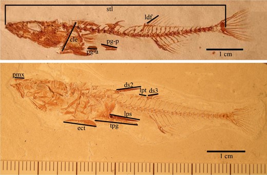
Phenotypes of a weakly armoured (above; 2 dorsal spines, vestigial pelvis) and strongly armoured (3 dorsal spines, full pelvis, first dorsal spine is indicated by an impression). Abbreviations: cleithrum (cle), dorsal fin ray (ldf), 2nd dorsal spine (ds2), 3rd dorsal spine (ds3), ectocoracoid (ect), pelvic girdle (tpg), pelvic girdle, anterior vestige (pg‐a), pelvic girdle, posterior vestige (pg‐p), pelvic spine (lps), premaxilla (pmx), pterygiophore (lpt), standard length (stl)
Trait definitions and functions: A, armour; L, locomotion; T, trophic
| Trait name | Function | Trait code | Trait description |
| Standard length | T | stl | Anterior tip of premaxilla to posterior end of hypural plate (i.e. last vertebra) |
| Premaxilla | T | pmx | Ascending process, from anterior tooth‐bearing tip to distal tip of the ascending process |
| Ectocoracoid | L, Aa | ect | Anterior to posterior tip |
| Cleithrum | L, Ta | cle | Dorsal to ventral tip |
| Dorsal fin ray | L | ldf | Base to tip of most anterior ray |
| Pterygiophore | A | lpt | Anterior to posterior tips of the pterygiophore immediately preceding the 3rd dorsal spine |
| Pelvic girdle | A | tpg | Anterior to posterior tips along midline. If vestigial, sum of longest anterior–posterior axis of the vestiges on one side |
| Pelvic spine | A | lps | Base of one pelvic spine to its distal tip |
| Dorsal spine 2 | A | ds2 | Anterior base of spine to its distal tip |
| Dorsal spine 3 | A | ds3 | Anterior base of spine to its distal tip |
Bones often do more than one thing. For example, the ectocoracoid is the lower border of the fossa for the pectoral musculature and its length is probably correlated with the size of the pectoral fin, which is longer in anadromous fish than benthic lake fish; however, the ect also protects the ventral area from predators and resists compression by predators. Similarly, the cleithrum is a measure of body depth and therefore indicates locomotion, but the lower end is also the origin of the abductor system for the lower jaw.
Pelvic girdle length (tpg) was a single measurement in specimens with the ancestral, complete pelvic girdles, but if the girdle was vestigial and expressed as separate anterior and posterior elements, then pelvic girdle length was the sum of the anterior and posterior vestige lengths (tpg = pg‐a + pg‐p). Often, only the anterior vestige was present, and it was treated as pelvic girdle length (pg‐a = tpg). Standard length was our measure of size, and we attempted to exclude the effects of pmx protrusion or taphonomic separations between vertebra on stl (Figure 1). Standard length in specimens with pronounced vertebral curvature was measured in two or three straight segments to limit the effect of curvature.
This set of ten bones was selected to capture variation in trophic morphology, body shape and armour. Individual bones were used as proxies for conventional, functionally relevant measurements (e.g. cle for body depth) because measurements that incorporate multiple bones are commonly distorted by displacement between them during fossilization.
Because armour traits are easiest to classify and the largest category, we categorized traits as armour (dorsal spines 1 and 2, pelvic spine, pterygiophore, pelvic girdle) or not (cleithrum, dorsal fin, ectocoracoid, premaxilla). We did this to observe whether allometric evolution was different for traits known to be under strong directional selection (armour), relative to those for which the selective regime is less clear (i.e. trophic, locomotory). Armour reduction evolved rapidly under directional natural selection within the time interval spanned by temporal sequence K (Hunt et al., 2008; Stuart et al., 2020). If the allometric relationship for armour traits is strong and constrained from evolving, then we would expect substantial body size evolution during armour loss. On the contrary, if allometric evolution is not constrained, then armour should be free to evolve without indirect, pleiotropic effects on size and other traits.
We used only the first 10 samples of temporal sequence K (i.e. the 10 oldest samples) because they provided the largest samples across all of the traits (Table 2). After sample 10, loss of armour traits frequently generates missing data for the lengths of the pelvic girdle and spine and dorsal spines.
Sample sizes by trait and stratigraphic sample
| Mean age | 0 | 268 | 1272 | 2201 | 3129 | 4073 | 5730 | 5960 | 6826 | 8501 |
| stl | 43 | 41 | 50 | 41 | 46 | 48 | 67 | 54 | 42 | 33 |
| pmx | 37 | 31 | 44 | 34 | 39 | 40 | 57 | 49 | 39 | 19 |
| ect | 32 | 34 | 46 | 37 | 31 | 43 | 60 | 52 | 39 | 22 |
| cle | 13 | 21 | 40 | 30 | 30 | 39 | 44 | 43 | 23 | 15 |
| ldf | 11 | 7 | 40 | 30 | 37 | 39 | 49 | 35 | 22 | 29 |
| lpt | 42 | 41 | 50 | 41 | 46 | 48 | 64 | 55 | 39 | 30 |
| tpg | 41 | 35 | 43 | 39 | 43 | 48 | 62 | 51 | 39 | 32 |
| lps | 42 | 40 | 44 | 41 | 43 | 41 | 23 | 30 | 7 | 5 |
| ds2 | 41 | 38 | 42 | 26 | 20 | 12 | 10 | 12 | 5 | 16 |
| ds3 | 41 | 40 | 50 | 41 | 45 | 43 | 63 | 48 | 37 | 29 |
Mean age is the average time of deposition in years for specimens in each sample, starting from the earliest sample (0 years) to the latest sample (8501 years).
The amount of time between the first and last specimens in each sample ranges from one year (a mass mortality event) to ca. 300 years. The relative mean time of deposition of specimens from each sample is presented in Table 2, and the time between the first and tenth samples was 8501 years.
Analysis
Static allometry
We chose to study bivariate allometry and not use multivariate approaches for two reasons, one biological and one technical. First, the bivariate tradition is well connected to the study of allomety sensu Huxley (Pélabon et al., 2014) and the study of allometries as potential constraints on trait evolution (reviewed in Voje et al., 2014). Second, as is typical for fossils, our data matrix had extensive missing data. Multivariate approaches like principal component analysis require complete data matrices, which would have necessitated either substantial sample size reduction or data imputation from a sparse matrix. Data imputation would have been further complicated by the fact that some missing data are supposed to be missing, due to the evolution of armour loss.
We natural log (ln) transformed standard length and then mean‐centred these values separately for each sample in the temporal sequence. We regressed ln‐transformed bone lengths on mean‐centred, ln‐standard lengths using ordinary least squares regression (OLS). The slopes and intercepts from these regressions estimate parameters a and b of the allometric equation described above. Note that regressing a trait on the mean‐centred standard length using OLS makes the estimated intercept parameter, a, equal to the trait's mean for a sample, thus giving the intercept a more intuitive biological interpretation (Gould, 1971; White & Gould, 1965). Mean‐centring standard length removes the inherit negative correlation between changes in intercept and slope. As such, the intercept is free to vary, and mean‐centring standard length does not hinder the study of intercept evolution (Egset et al., 2012).
Variance of allometric parameters
We tested for change in static allometric slopes using phylogenetic mixed‐effect models, regressing ln(trait) on ln(standard length) with sample as a random factor, fitted using the R package mcmcglmm (Hadfield, 2010). We compared a model that assumed a fixed allometric slope common to all samples to a second model that allowed the slopes to vary among samples. Each Markov chain Monte Carlo (MCMC) model ran for 200 000 iterations, with a burn‐in of 100 000 and a thinning interval of 200 iterations. The priors for the variances in the mixed models were set to an inverse‐Gamma (V = 1, nu = 0.002). These priors are often used for variance components, and we note that the estimated model parameters were not sensitive to changes in these priors (preliminary results not shown). We evaluated MCMC chain mixing by inspecting trace plots, investigating the autocorrelation of samples and examining convergence using Heidelberger and Welch's MCMC Convergence Diagnostic (reported in Table S2; Heidelberger & Welch, 1981, 1983). Because the temporal sequence studied here is a set of samples presumably taken from the same lineage at different times, we accounted for phylogenetic dependency in the data by adding phylogenetic relatedness as a random effect. We created a phylogeny of the samples using the R package phytools (Revell, 2012) where the fossil samples branched from the stem at intervals corresponding to the time separating the mean ages of the samples (first row of Table 2). Each branch to a fossil sample was given a length of 1 year (Figure S1). We used DIC (Spiegelhalter et al., 2002) to compare models and accepted a difference of 2 units as evidence for a better model. We interpreted superiority of the variable‐slope model as evidence for true changes in static slopes through time.
A close match between static and evolutionary exponents is predicted if static allometry influences phenotypic divergence. We estimated evolutionary allometries by regressing mean (ln‐transformed) bone lengths for each sample on mean (ln‐transformed) standard lengths within each sample using ordinary least squares regression (OLS). We assessed alignment of evolutionary allometry and the single‐sample static allometries (from OLS) by calculating the difference between the evolutionary allometric slope and the mean of the static slopes among samples, for each trait.
Pattern of evolution in body size and in allometric parameters
The pattern of allometric slope evolution can indicate whether changes in slopes show a trend or just fluctuations around a mean. We investigated the pattern of body size evolution and allometric parameters by fitting four evolutionary models to observed change through time in ln‐standard length and each trait's static allometric parameters through time (from OLS). We used the R package paleoTS v.0.5.2 (Hunt, 2006; Hunt et al., 2008, 2015). The models were directional change, random walk, stasis (white noise) and strict stasis (trait evolution explained by sampling variance alone). Recall that we mean‐scaled our data within each fossil sample before fitting the allometric model using OLS. Thus, the intercept estimate is the same as the trait mean and the best fit models for changes in intercepts accordingly describe evolution of the trait means. We did not fit an Ornstein–Uhlenbeck model to these data (e.g. did not follow Hunt et al., 2008) because we did not want to fit a model with four parameters to a data set with only 10 samples. Hunt et al. (2008) had three traits sampled from the same section at 250‐year resolution and therefore had four times as many samples to fit and distinguish among models. (We note that this issue of power to distinguish among models applies also to the trend model (three parameters), relative to stasis (two parameters), random walk (two parameters) and strict stasis (one parameter).) We used the fit4models function, specifying the joint parameterization option. We assessed relative model fit using Akaike weights (ωi) calculated from the small‐sample‐corrected Akaike information criterion values (AICc) output by paleoTS. ωi is roughly the conditional probability that a given model is best among the candidate models (Symonds & Moussalli, 2011).
Correlated evolution of allometric parameters
If traits are genetically correlated, then the evolution of their static allometric slopes might not be independent. For each trait, therefore, we calculated consecutive changes in static allometric slope through time (10 samples = 9 changes) and computed how changes in slopes correlated among traits. To assess the effect of sampling error on these correlations, (i.e. whether the observed correlations are outside the distribution of correlations computed for random vectors with independent, uncorrelated elements), we (i) simulated two vectors of length 10 where the elements were drawn from a multivariate normal distribution with a mean 0, a variance of 0.3 (similar to the observed variance in slopes and intercepts) and a covariance of 0, (ii) calculated the correlation between the elements in the two vectors and (iii) repeated this procedure 10 000 times. Observations outside the 95th percentile of the 10 000 correlations (0.56) were deemed greater than what we would expect due to sampling error alone.
Contributions of change in body size and allometric parameters to trait evolution
Under the logarithmic (and thus linear) version of the allometric model described above, changes in the trait mean (y) in a population across time result from a combination of changes in the intercept (a) and the interaction between changes in body size and the allometric slope (b). The relative contribution of changes in body size, intercept and slope to changes in the trait mean (i.e. the variance in trait means across time) can be quantified by calculating the trait variance conditional on different allometric parameter combinations (Voje et al., 2014). As changes in slope, intercept and body size are on different scales, their relative contribution to changes in trait means cannot be compared directly (Voje et al., 2014). Instead, the conditional variance method converts changes in slope, intercept and body size to a common currency: predicted trait variation (Voje et al., 2014). A substantial reduction of the estimated variance in trait means after conditioning on a given parameter indicates that a change in that parameter played a major role in trait evolution. For example, if the variance in the trait means among the ten samples is gone when conditioning this variance on observed variance in body size, this suggests the evolution of the trait mean can be explained by changes in body size alone. In contrast, if size or an allometric parameter (or parameter combination) has a weak association with variation in a trait through time, then change in that parameter (or combinations of parameters) has not contributed much to the evolution of the trait.
According to the allometry‐as‐constraint hypothesis, we expect that the evolvability of the allometric slope is low relative to evolvability of body size and the allometric intercept. That is, if the hypothesis is true, then we expect any evolved variation in slope to explain little of the variation in trait mean. Rather, most of the conditional variance would be explained by changes in allometric intercept or body size because the relationship between trait and size (i.e. allometric slope) will have stayed roughly constant during evolution.
The formulae to calculate the relevant conditional variances for the allometric model were given in Table 1 of Voje et al. (2014), but here we introduce an R package called allometry to calculate the conditional variances (github.com/klvoje/allometry). Prior to this analysis, the means of body size among samples are centred at zero (i.e. the average of all average body sizes among samples is zero). Note that this centring of the means of body size among samples is not equivalent to centring the body size variable around zero within each sample, as we did when estimating the intercepts using OLS. The intercepts in this analysis are therefore not the same as the ones estimated using OLS, and they are not identical to the trait mean in each sample. Furthermore, we also assumed that the parameters (i.e. intercept, slope and body size) follow a multivariate normal distribution (Voje et al., 2014).
allometry functions allow calculation of the per cent predicted trait variance that remains after body size, intercept, slope or combinations of those parameters (i.e. size and intercept, size and slope, intercept and slope) are held constant. The amount of (residual) variance for the trait after conditioning on a parameter (or combination of parameters) indicates the parameter(s)'s relative importance in explaining changes in trait means through time. Lower residual variances imply greater importance. In the context of this study, the trait variance is the variance of the trait means among fossil samples. However, trait variance can also represent variance among extant populations or species, which is how the method was originally used by Voje et al. (2014).
RESULTS
Evolution of body size and static allometric intercepts
Body size varied through time (Figure 2), though the best evolutionary model for that change was stasis (Table 3), suggesting that body size responded to fluctuating selection through time. We found evidence for variation in all static allometric intercepts (i.e. trait means); the 95% confidence intervals about these parameter estimates never included 0 (Table 4, Figure 3).
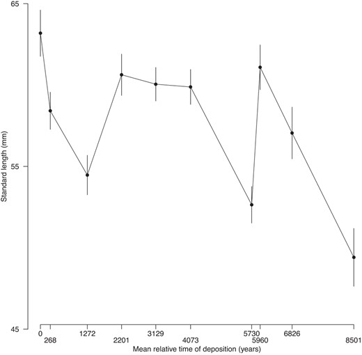
Means of standard length against sample mean relative time of deposition. Error bars are standard errors
Evolution of mean size and allometric intercepts (i.e. trait means) is mostly consistent with overall stasis or random walks
| Trait | ωi Trend | ωi Random walk | ωi Stasis | ωi Strict stasis |
| stl | 0.021 | 0.130 | 0.849 | 0.000 |
| pmx | 0.041 | 0.256 | 0.703 | 0.000 |
| ect | 0.043 | 0.267 | 0.689 | 0.000 |
| cle | 0.012 | 0.082 | 0.906 | 0.000 |
| ldf | 0.123 | 0.641 | 0.236 | 0.000 |
| lpt | 0.686 | 0.314 | 0.000 | 0.000 |
| tpg | 0.266 | 0.733 | 0.001 | 0.000 |
| lps | 0.277 | 0.719 | 0.004 | 0.000 |
| ds2 | 0.354 | 0.645 | 0.000 | 0.000 |
| ds3 | 0.278 | 0.717 | 0.005 | 0.000 |
Here, we report Akaike weights (ωi), which are roughly indicative of the probability that a given model is the best model. Bold indicates the best model.
Evidence for evolution of static allometric slopes and intercepts
| Trait | Slope variance (95% CI) | Intercept variance (95% CI) | Mean R2 | Minimum R2 | ΔDIC | Δslope |
| pmx | 0.153 (0.042–0.315) | 0.561 (0.076–1.362) | 0.570 | 0.181 | −5.07 | −0.305 |
| ect | 0.148 (0.045–0.308) | 0.502 (0.094–1.114) | 0.642 | 0.468 | −13.49 | −0.448 |
| cle | 0.150 (0.045–0.313) | 0.523 (0.090–1.185) | 0.643 | 0.412 | −13.64 | −0.298 |
| ldf | 0.153 (0.042–0.318) | 0.578 (0.097–1.298) | 0.543 | 0.342 | −13.31 | −0.711 |
| lpt | 0.176 (0.041–0.373) | 0.932 (0.089–2.292) | 0.220 | 0.002 | −10.23 | −1.263 |
| tpg | 0.176 (0.044–0.380) | 0.806 (0.076–2.139) | 0.360 | 0.000 | −2.88 | −4.217 |
| lps | 0.158 (0.046–0.334) | 0.582 (0.080–1.440) | 0.226 | 0.003 | −4.66 | −2.000 |
| ds2 | 0.149 (0.044–0.312) | 0.411 (0.066–1.000) | 0.198 | 0.006 | −0.60 | −1.485 |
| ds3 | 0.144 (0.039–0.302) | 0.379 (0.066–0.894) | 0.141 | 0.000 | 0.94 | −1.710 |
Among‐sample variances (95% CI) of the allometric slope and intercept are from the random‐slope random‐intercept mixed model. Mean and minimum R 2 are the average and the minimum of the R 2 values from OLS regressions to estimate the parameters of the allometric model in the ten samples. ΔDIC compares a GLMM model that allows static slopes to vary across samples versus a model where static slope is fixed. Negative ΔDIC values smaller than −2.0 favour the variable‐slope model. Δslope is the difference between the average static slope and the evolutionary (among‐sample) allometric slope. Negative Δslope values indicate that the evolutionary allometry is steeper than the average static slope.
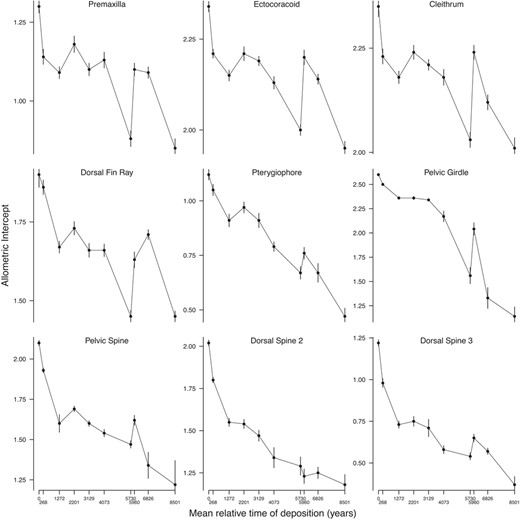
Allometric intercepts through time. For each sample, the intercept and standard error estimated by the allometric model are plotted Since the intercepts were calculated on mean‐centred data, these plots can be interpreted as change of trait mean through time
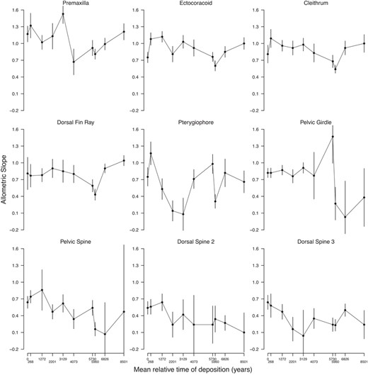
Evolution of static allometric slopes
The variable‐slope model was clearly favoured over the fixed slopes model for seven out of nine traits per DIC, suggesting that these allometric slopes contain variation that cannot be explained by sampling error alone. The exceptions were for the second and third dorsal spine length (Table 4). Slopes for the dorsal spine lengths showed best relative fit to the strict stasis model (Table 5). Thus, observed differences in slopes across time for both dorsal spines may be explained by sampling variance alone. Also changes in the slope of the pelvic girdle length were best fit by a strict stasis model (Table 5). Therefore, although it is possible that some evolution has occurred in the static allometric slopes of the pelvic girdle, we do not consider the evidence to be particularly convincing (Figure 4).
Evolution in allometric slopes is mostly consistent with fluctuating evolution but overall stasis
| Trait | ωi Trend | ωi Random walk | ωi Stasis | ωi Strict stasis |
| pmx | 0.028 | 0.232 | 0.439 | 0.301 |
| ect | 0.023 | 0.189 | 0.683 | 0.105 |
| cle | 0.043 | 0.368 | 0.567 | 0.022 |
| ldf | 0.037 | 0.281 | 0.658 | 0.025 |
| lpt | 0.007 | 0.057 | 0.886 | 0.050 |
| tpg | 0.021 | 0.140 | 0.140 | 0.699 |
| lps | 0.476 | 0.276 | 0.124 | 0.124 |
| ds2 | 0.172 | 0.200 | 0.105 | 0.523 |
| ds3 | 0.086 | 0.187 | 0.160 | 0.566 |
Again, we report Akaike weights (ωi). Bold indicates the best model.
Allometric slopes through time. For each sample, the slope and standard error estimated by the allometric model are plotted
In contrast to the three traits presented above, there is consistent evidence that the static slopes of the other six traits varied through time (Tables 4 and 5). However, pterygiophore length and pelvic spine length showed, on average, a low correlation with body size and had at least one sample for which this correlation was effectively zero (Table 4). One interpretation of this low—and even absent—correlation with body size is that the allometric model does not fit these traits well. That is, there is no convincing allometric relationship between body size and these traits (low R 2 values in Table 4). As such, pterygiophore and pelvic spine (as well as girdle length and the second and third spine lengths, Table 4) might not be relevant to our question of how fast static allometry evolves because there is no substantial allometric relationship to evolve in the first place. Therefore, we are left with four traits (premaxilla length, cleithrum length, ectocoracoid length and dorsal fin length) that each showed a consistent fit to the allometric model within each time interval (relatively high R 2 values in Table 4) and also have evidence for evolving slopes (Figure 4, Tables 4 and 5). Slope evolution for these four traits showed best relative fit to the stasis model (Table 5), indicating fluctuating but little net evolutionary change across 8500 years. The evolution of static slopes is correlated for some of these traits, including ectocoracoid, cleithrum and dorsal fin lengths (Table 6).
Correlations for changes in slopes (above diagonal) and intercepts (below diagonal) through time
| pmx | ect | cle | ldf | lpt | tpg | lps | ds2 | ds3 | |
| pmx | ‐ | 0.35 | 0.48 | 0.17 | −0.10 | 0.31 | 0.47 | 0.19 | −0.55 |
| ect | 0.85 | ‐ | 0.79 | 0.38 | 0.37 | 0.18 | 0.59 | 0.46 | 0.19 |
| cle | 0.82 | 0.68 | ‐ | 0.71 | 0.46 | 0.05 | 0.23 | 0.01 | 0.19 |
| ldf | 0.22 | 0.23 | 0.37 | ‐ | 0.22 | −0.02 | −0.01 | −0.38 | 0.23 |
| lpt | −0.15 | −0.28 | 0.02 | 0.18 | ‐ | 0.35 | 0.12 | −0.13 | 0.62 |
| tpg | 0.25 | 0.16 | 0.54 | −0.18 | 0.14 | ‐ | 0.74 | −0.11 | −0.31 |
| lps | −0.04 | −0.05 | 0.28 | −0.03 | 0.05 | 0.00 | ‐ | 0.34 | −0.33 |
| ds2 | 0.56 | 0.60 | 0.56 | 0.17 | −0.51 | 0.08 | 0.25 | ‐ | 0.14 |
| ds3 | 0.04 | −0.10 | 0.01 | 0.54 | 0.62 | −0.53 | 0.17 | −0.09 | ‐ |
Values in bold are above the threshold expected based on sampling error alone (see text for more details).
Alignment of static and evolutionary slopes
For each of the nine traits, the slope of the OLS regression for trait means upon mean size (i.e. the among‐sample, evolutionary allometric slope) deviates from the mean of the static allometric slopes averaged across samples (Figure 5, Table 4). The deviation between average static and evolutionary allometric slope is less for the non‐armour traits showing a consistent fit to the allometric model in all samples (i.e. lengths of the premaxilla, ectocoracoid, cleithrum and dorsal fin).
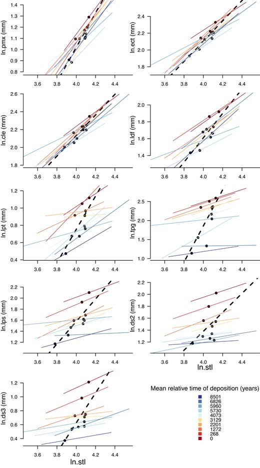
Static allometric relationships by trait by sample (thin black lines). Evolutionary allometric relationship is the OLS fit line through the sample means (heavy broken line). Axes are on a log (ln) scale. The top four traits are non‐armour traits. The bottom five traits are armour traits. Colour shows relative time of deposition, with blues being younger (time goes forward from red to blue)
Contributions of body size and allometric parameters to trait evolution
Variance in slope values across samples accounted for little of the variance in trait means across samples, relative to the contribution of variance in intercept and body size (Table 7). Thus, despite evidence for some evolution in static slope in four of the traits (i.e. the premaxilla, cleithrum, ectocoracoid, dorsal fin), these changes in scaling had almost no effect on trait evolution in the lineage. In contrast, only a few per cent of the variation was left in trait means when they were conditioned on both intercept and body size (median % variance remaining = 0.6; Table 7).
Per cent of the predicted variance among sample means that remains when conditioning on size, static allometric intercept and static allometric slope (or their combinations)
| pmx | ect | cle | ldf | lpt | tpg | lps | ds2 | ds3 | |
| Size | 25.1 | 16.90 | 20.00 | 42.10 | 42.40 | 42.50 | 45.90 | 68.10 | 50.60 |
| Intercept | 44.1 | 24.10 | 36.60 | 14.50 | 5.30 | 0.80 | 1.50 | 0.90 | 1.00 |
| Slope | 76.8 | 59.30 | 69.10 | 66.80 | 73.90 | 70.80 | 60.60 | 38.00 | 57.20 |
| Allometry | 44.1 | 19.20 | 34.80 | 11.70 | 4.40 | 0.50 | 0.80 | 1.00 | 0.90 |
| Intercept + Size | 2.5 | 1.00 | 1.50 | 0.60 | 1.80 | 0.20 | 0.20 | 0.10 | 0.20 |
| Slope + Size | 22.3 | 13.90 | 18.10 | 33.10 | 38.40 | 24.10 | 17.20 | 33.10 | 28.70 |
DISCUSSION
To what extent is allometry evolvable and does allometry constrain phenotypic divergence? These questions have generally been investigated using samples from extant, conspecific populations and species spanning either generational or macroevolutionary timescales. Here, we studied the evolution of static allometries of nine traits in a fossil stickleback lineage across 8500 years to investigate the tempo and mode of allometric evolution at a time scale that is intermediate between generational and macroevolutionary time scales. We also explored how evolvability of static allometry interacts with trait evolution.
In this system, trait means were known to evolve (Bell, 2009; Bell et al., 1985, 2006; Hunt et al., 2008; Stuart et al., 2020). At least three armour traits of this stickleback lineage experienced directional natural selection for reduction in this sequence (Hunt et al., 2008; Stuart et al., 2020). The armour traits in this sequence also showed a relatively poor fit to the allometric model, with mean R 2 values for all five traits across all samples ranging from 0.14 to 0.36 (Table 4) (although measurement error also contributes to the low R2). The observed mixed evidence for constraint is therefore difficult to interpret since allometric relationships were weak to begin with: at the same time as variation in static slopes contributed almost nothing to trait evolution, we also found that the static allometric slopes were poor predictors of the evolutionary allometries. We therefore conclude that allometry is probably not acting as a constraint on phenotypic diversification in armour traits. Perhaps a weak allometric relationship evolved in the lineage, precisely because strong directional natural selection for armour gain and loss had been regular feature of G. doryssus phylogeny, as follows.
Evolution of the closely related, extant Threespine Stickleback Gasterosteus aculeatus is remarkable in part for the repeated, independent reduction of armour in derived freshwater populations, relative to their marine ancestors. Armour evolution appears to be driven by two sources of selection—the physiological cost of building bone and predation defence. The strength and direction of selection from each source depends on whether the habitat is marine or freshwater and on the predation regime. Marchinko and Schluter (2007) showed experimentally that individuals with complete lateral armour plating grew more slowly than low‐plated individuals in freshwater, but that there was no difference when they developed in saltwater. This indicated that selection should favour armour loss in freshwater, where bone‐building minerals can be limiting (see also Giles, 1983; but see Rollins et al., 2014). Yet, bony armour makes it more likely that stickleback escape piscivorous vertebrate predators in both marine and freshwater habitats (Reimchen, 1994, 1995; Vamosi & Schluter, 2002). Thus, in marine environments, where vertebrate piscivores and bone‐building minerals are common, selection for armour by predators should be stronger, and oceanic Threespine Stickleback are highly armoured (Jamniczky et al., 2018). In freshwater, vertebrate piscivores are less common, and armour's physiological cost is greater, thereby driving armour loss (Hagen & Gilbertson, 1973; Reimchen, 1994, 1995, 2000; Vamosi & Schluter, 2002). Moreover, even variation in predation among freshwater habitats causes variation among populations for armour. For example, in replicate lakes that contain both littoral benthic and open‐water limnetic ecotypes, limnetics are more armoured than benthics (McPhail, 1994; Schluter & McPhail, 1992; Vamosi & Schluter, 2002), though both ecotypes are less armoured than marine stickleback. Predation experiments and comparative studies have shown that limnetic individuals are exposed to higher rates of trout predation, creating divergent selection that causes limnetic stickleback to retain more armour than benthics (Vamosi & Schluter, 2002, 2004). Selection for armour loss in freshwater may even be further enhanced if piscivorous insects, which apparently can use armour to grasp fish during capture, are present in benthic microhabitats (Marchinko, 2009; Reimchen, 1994). In sum, in G. aculeatus, selection appears to favour armour reduction in freshwater. Why would this cause evolution of weak allometric relationships between armour and size?
Size affects most aspects of an organism's biology. As such, evolutionary changes in size are likely to alter feeding, swimming, predation, growth, life history and other traits. If armour traits and size were strongly correlated (i.e. a tight allometric slope), then strong selection to evolve armour would result in correlated evolution of body size and ecologically important traits that vary with size. It stands to reason then that individuals with stronger allometric relationships between armour and size might be more likely to experience negative indirect effects when the rest of their body plan changes during armour evolution. Accordingly, weaker allometry of armour traits would be favourable in freshwater. Indeed, armour phenotypes of extant Threespine Stickleback tend to be polygenic, and the genes for them tend to be unlinked (Colosimo et al., 2004; Cresko et al., 2004; Howes et al., 2017; Indjeian et al., 2016; Roberts Kingman et al., 2021; Roberts Kingman et al., 2021; Shapiro et al., 2004). This genetic architecture could spread geographically during gene flow between marine and freshwater fish (the transporter hypothesis; Jones et al., 2012; Roberts Kingman et al., 2021; Schluter & Conte, 2009) and become a general characteristic of the species.
If these inferences are correct, we speculate that similar evolution would have been occurring for G. doryssus. If directional selection on armour produced maladaptive change in non‐armour traits through their genetic correlations with size (i.e. allometry), then the response to such selection could be impeded, reducing local adaptation to the predation regime. Selection would therefore have favoured individuals with weaker pleiotropic relationships between body size and armour traits. A weak relationship would have evolved and spread across a landscape with variable predation regimes. As such, adaptive armour evolution in the lineage we studied could have proceeded quickly, with little constraint from trait‐body size relationships. This is consistent with studies in extant G. aculeatus that have found minimal evidence for genetic constraint during adaptation to freshwater (Walker & Bell, 2000; Aguirre & Bell, 2012; but see Schluter, 1996; Hansen & Voje, 2011).
In contrast, the four non‐armour traits fit the static allometric model better: mean R 2 values across 10 samples for those four traits range from 0.54 to 0.64 (Table 4). These results suggest that armour phenotypes developed more independently with respect to body size than the non‐armour traits during the time span studied here. We found evidence for evolution of static allometric slopes of non‐armour traits (Tables 4 and 5). Although this evolution was not large and the direction of change varied (Table 5), the time scale on which we detected change was two orders of magnitude less than the one fossil case in which static allometric slope evolution has been observed. Wei (1994) detected evolution of static allometric slope of the foraminiferans Globoconella inflatus and G. puncticulata across 2–3 million years. Wei's (1994) study focussed on the effect of heterochronic changes to morphological evolution and did not explicitly study the evolvability of the allometric exponent. However, when we reanalysed the static slopes reported in Wei's (1994) Table 4 by subtracting the mean of the squared standard errors of the slopes from the variance in static slopes, we observed corrected standard deviations in the slope estimates of 0.13 for G. puncticulata and 0.38 for G. inflatus. These positive values imply evolutionary changes in slopes. Thus, although some of the slope variance that we observed could be explained by phenotypic plasticity (Stamp & Hadfield, 2020), effects of time‐averaging (Hunt, 2004a, 2004b) and other causes, a reasonable interpretation of our study is that static slopes can evolve on 1000‐year timescales. Purnell et al. (2007) showed that during the period that we studied, this G. doryssus lineage evolved changes in tooth wear that indicated a shift from benthic feeding to planktivory. Such a dietary shift should cause directional selection on jaw morphology and swimming traits (McGee et al., 2013; McPhail, 1994; Schluter & McPhail, 1992), which might drive changes in allometric relationships. Thus, our findings are consistent with the hypothesis that selection can shape allometric relationships on relatively short periods of time.
However, for several reasons, we caution against an inference that allometric slopes did not constrain non‐armour trait evolution in G. doryssus. First, observed variation in static slope values was small and fluctuated (Figure 3, Table 5), often departing little from white noise (i.e. stasis), even in a system with strong directional selection on trait values. Second, relative change in slope values through time was much smaller than change in intercepts. In other words, trait means (i.e. the intercept) seem to be more evolvable than the developmental relationship between the traits and size. Thus, it still appears that static slopes are less evolvable than other quantitative traits. Unfortunately, our data do not suffice to distinguish how pleiotropy and stabilizing selection might each contribute to the low evolvability of the allometric slopes observed here (Armbruster & Schwaegerle, 1996; Arnold et al., 2001, 2008; Bolstad et al., 2015; Gould, 1966, 1977, 2002; Houle et al., 2019; Huxley, 1932; Klingenberg, 2005; Lande, 1985; Maynard Smith et al., 1985; Pélabon et al., 2014; Savageau, 1979; Stevens, 2009).
CONCLUSION
In this lineage of G. doryssus, non‐armour traits had stronger static allometric relationships and less deviation between static and evolutionary allometries through time, compared to armour traits (Figure 5, Table 4). Moreover, in non‐armour traits, the observed variance in static slope across samples accounted for a negligible amount of the observed variance in trait means, and the static slopes of non‐armour traits remained sufficiently stable to influence the direction of phenotypic diversification predictably.
In contrast, armour traits had much weaker allometric relationships in the first place and had greater deviations between static and evolutionary allometries. This suggests armour trait evolution was not constrained by allometry, perhaps because previous, strong selection on armour during ancient, repeated colonization of freshwater (Nelson & Cresko, 2018; Schluter & Conte, 2009) weakened the developmental genetic relationships between armour and body size in Threespine Stickleback.
ACKNOWLEDGEMENTS
We thank the same organizations and people acknowledged in Stuart et al. (2020). We thank M.P. Travis for specimen photography, morphological data collection and counting annual laminations. This research was supported by NSF grants BSR‐8111013, EAR‐9870337 and DEB‐0322818, the Center for Field Research (Earthwatch), the National Geographic Society (2869‐84), and NIH grant GM124330‐01 to M.A. Bell and by NSF grant DEB‐1456462 to Y.E. Stuart. KLV is supported by an ERC‐2020‐STG (Grant agreement ID: 948465).
CONFLICTS OF INTEREST
The authors have no interests or relationships, financial or otherwise, that influence our objectivity.
AUTHOR CONTRIBUTIONS
YES and KLV designed the research, analysed data and created figures. MAB supervised sample and data collection. KLV wrote the R package. YES and KLV wrote the paper. All authors jointly edited the paper.
PEER REVIEW
The peer review history for this article is available at https://publons.com/publon/10.1111/jeb.13984.
OPEN RESEARCH BADGES
This article has earned an Open Data, for making publicly available the digitally‐shareable data necessary to reproduce the reported results. The data is available at https://doi.org/10.5061/dryad.5qfttdz76.
DATA AVAILABILITY STATEMENT
The data, R code and information necessary to recreate the analyses in this article will be archived at datadryad.org: https://doi.org/10.5061/dryad.5qfttdz76.
REFERENCES
