


Abstract
Our ability to examine genetic variation across entire genomes has enabled many studies searching for the genetic basis of local adaptation. These studies have identified numerous loci as candidates for differential local selection; however, relatively few have examined the overlap among candidate loci identified from independent studies of the same species in different geographic areas or evolutionary lineages. We used an allelotyping approach with a 220K SNP array to characterize the population genetic structure of Atlantic salmon in north‐eastern Europe and ask whether the same genomic segments emerged as outliers among populations in different geographic regions. Genome‐wide data recapitulated the phylogeographic structure previously inferred from mtDNA and microsatellite markers. Independent analyses of three genetically and geographically distinct groups of populations repeatedly inferred the same 17 haploblocks to contain loci under differential local selection. The most strongly supported of these replicated haploblocks had known strong associations with life‐history variation or immune response in Atlantic salmon. Our results are consistent with these genomic segments harbouring large‐effect loci which have a major role in Atlantic salmon diversification and are ideal targets for validation studies.
Abstract

INTRODUCTION
Technological advances enabling variation to be examined across entire genomes have enabled many studies searching for the genetic basis of local adaptation. These studies, which commonly examine a collection of populations for the genomic signatures of selective sweeps or the presence of polymorphisms that co‐vary with environmental parameters, have identified a myriad of loci as ‘candidates’ to underlie adaptive phenotypes (Haasl & Payseur, 2015; Hoban et al., 2016). Fewer studies, however, have investigated the extent of overlap among candidate loci across independent studies of the same species in different geographic areas or evolutionary lineages. Examining such overlap can provide important insights into the evolutionary process, in particular allowing us to ask whether the same genetic architecture repeatedly underlies adaptative diversification (e.g. Ravinet et al., 2015; Roesti et al., 2012; Turner et al., 2018; Yeaman et al., 2018), and whether this architecture includes loci of large effect (Oomen et al., 2020). Further, from a technical point of view, the rate of false‐positive candidates in a single study can be high (François et al., 2016; Lotterhos & Whitlock, 2015; Weigland & Leese, 2018). Loci that are repeatedly identified as locally adaptive candidates in replicated or complementary analysis of independent data sets (e.g. Buehler et al., 2014; Liu et al., 2014; Rellstab et al., 2015) are more likely to be true positives that are important in adaptive diversification for the species as a whole. Such loci are ideal targets for further research aimed at validating their adaptive importance by quantifying their phenotypic consequences and characterizing their effect on fitness in different environments, and ultimately understanding their population genetic history and evolutionary significance.
Salmonid fishes, including the anadromous and potadromous Atlantic salmon (Salmo salar), typically show strong population genetic subdivision due to their precise natal homing and/or isolation in different bodies of water (reviewed in Fraser et al., 2011). They also exhibit a wide range of life‐history variation within and across populations, including differences in age at sexual maturity, migration timing and breeding location, and exploitation of ecological niches (e.g. Bernatchez et al., 2010; Dodson et al., 2013; Quinn et al., 2016). These properties, together with the excellent genomic resources available for the taxon, have made salmonid fishes important models for examining the genetic basis of phenotypic variation and local adaptation. Recent studies have identified three independent large‐effect loci that repeatedly underlie life‐history variation across salmonid populations and species (Ayllon et al., 2015; Barson et al., 2015; Hess et al., 2016; Prince et al., 2017; Veale & Russello, 2017). A small number of additional loci have been confirmed as strong candidates to underlie local adaptation across multiple populations (Larson et al., 2019; Pritchard et al., 2018). Nevertheless, most loci that have been identified as locally adaptive candidates in salmonids remain unique to a single study. There is a need to examine how many of these loci are of broader adaptive significance.
The native breeding range of Atlantic salmon spans the north Atlantic coast from eastern North America to western Russia. Populations are genetically structured at multiple spatial scales, which reflects long‐term isolation and post‐glacial recolonization processes. This structure ranges from extreme divergence between the North American and European lineages to fine‐scale differentiation between populations in different tributaries of the same river (e.g. Lehnert et al., 2019; Vähä et al., 2007; Wennevik et al., 2019). European Atlantic salmon have been separated into up to five major phylogenetic lineages, each with a distinct geographic range (Bourret et al., 2013; King et al., 2001; Rougemont & Bernatchez, 2018; Verspoor et al., 1999). The ‘Barents–White Seas’ lineage of Atlantic salmon is distributed across the contiguous subarctic regions of north‐eastern Norway, northern Finland and north‐western Russia (Figure 1; Bourret et al., 2013; Wennevik et al., 2019). Rivers in this region support some of the world's most important wild Atlantic salmon populations, which face ongoing threats including legal and illegal fishing pressure, the local expansion of salmon aquaculture, and changing environmental conditions (Ozerov et al., 2012; Primmer et al., 2006). Previous studies using allozymes, mtDNA and microsatellites have identified further substructure within the Barents–White Seas lineage. In particular, on the Russian Kola Peninsula, there is a clear genetic transition between Atlantic salmon spawning in rivers that open into the Barents Sea and those spawning in rivers that open into the White Sea (Asplund et al., 2004; Ozerov et al., 2017; Tonteri et al., 2009; Wennevik et al., 2019). This transition is associated with broad‐scale differences in life‐history parameters between the two regional groups including age at sexual maturity and timing of the return spawning migration (Jensen, 1999; Ponomareva, 2007; Potutkin et al., 2007). Many studies have also identified a second genetic transition between the White Sea populations that spawn in rivers on the Kola Peninsula and those spawning in rivers opening onto the south‐western White Sea in the Republic of Karelia (Asplund et al., 2004; Tonteri et al., 2009; but see Ozerov et al., 2017). This regional sub‐structuring is suggested to be the result of post‐glacial recolonization from multiple refugia. There is a consensus that the Barents region was re‐colonized from the eastern Atlantic—uniquely among European Atlantic salmon, the Barents populations also contain genetic signals consistent with gene flow from North America (Asplund et al., 2004; Bradbury et al., 2015; Makhrov et al., 2005). Salmon are suggested to have re‐colonized the White Sea from a north‐eastern glacial refugium (Asplund et al., 2004; Bourret et al., 2013; Tonteri et al., 2009) or alternatively from the Baltic via freshwater Lake Onega (Makhrov et al., 2005).
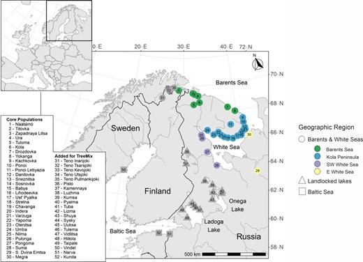
Map of the sampling locations. Colours indicate populations analysed in detail in this study, whereas grey indicates populations added for the TreeMix analysis. Different shapes represent major geographic regions (circles: Barents and White Seas, squares: Baltic Sea, triangles: landlocked freshwater locations), whereas colours indicate sub‐regions within the Barents and White Seas (green: Barents Sea; blue: Kola Peninsula; purple: South‐West White Sea; yellow: East White Sea). See Pritchard et al. (2018) for the sampling locations for the reanalysed Teno River data set
Recently, Pritchard et al. (2018) used a SNP array to scan for genomic signatures of differential local selection among 10 genetically distinct populations in the Teno (Tana/Deatnu) River, a drainage which supports a large, subdivided, Barents Sea Atlantic salmon stock. They examined patterns of interpopulation differentiation, allelic association with upstream catchment area and distance from the ocean, and local haplotype homozygosity, and identified 32 genomic segments as particularly strong candidates to contain locally adaptive variants. Here, we use the same SNP array to characterize population structure among 30 additional salmon populations from north‐eastern Europe, and ask whether the same genomic segments emerge as locally adaptive candidates between the different geographic regions.
MATERIALS AND METHODS
Data formatting and statistical analyses were performed either in R 3.5.1. (R Core Team, 2019), with assistance from functions in the tidyverse package (Wickham, 2016), or in the Linux shell.
Sample collection & DNA extraction
We used samples of Atlantic salmon that had been collected from 29 rivers in north‐eastern Russia and one river in north‐western Finland/Norway (Näätämö/Neiden/Njeävdám) between 1999 and 2008 (median sample size = 44 fish, range = 25–240; Table 1, Figure 1). All samples were obtained according to relevant national legislations. Most of these rivers are known to have temporally stable population genetic structure (Ozerov, Vasemägi, et al., 2013). Due to the late expansion of Atlantic salmon farming into this region, they are not expected to have contained genetic material from aquaculture strains at the time of sampling; however, several of the rivers including Kola and Umba have been subject to long‐term supplementary stocking programmes using locally caught broodstock (Makhrov et al., 2004). All Russian river samples were fin clips in ethanol from juvenile fish caught by electrofishing. Näätämö samples were dry scales taken from adult fish harvested in the river. DNA had previously been extracted from the samples using various methods (Ozerov et al., 2012; Pritchard et al., 2016; Zueva et al., 2014, 2018) and stored at −20ºC for several years. All archived DNA was qualitatively assessed for degradation using gel electrophoresis. For 618 degraded samples, DNA was freshly extracted from stored tissue using QIAamp DNA mini kits (Qiagen, Table 1).
Details of the studied Atlantic salmon populations: regional grouping, sample year and location, catchment area of the river, number of individuals pooled, and observed heterozygosity (H0). Population numbers match those in Figure 1
| Key | River | Region | Lat | Long | Catchment area (km2) | Sample year | DNA extracted | Pool size | Ho |
| 1 | Näätämo | Barents Sea | 69.7 | 28.98 | 2,962 | 2006–08 | 2012 | 4 x 60 | 0.316 |
| 2 | Titovka | Barents Sea | 69.48 | 31.82 | 1,226 | 2000 | 2006 | 38 | 0.343 |
| 3 | Zapadnaya Litsa | Barents Sea | 69.4 | 32.15 | 1688 | 2000 | 2015 | 43 | 0.348 |
| 4 | Ura | Barents Sea | 69.29 | 32.82 | 1,029 | 2000 | 2015 | 44 | 0.358 |
| 5 | Tuloma | Barents Sea | 68.67 | 31.94 | 18,231 | 1998 | 2015 | 40 | 0.352 |
| 6 | Kola | Barents Sea | 68.82 | 33.08 | 3,846 | 2000 | 2015 | 40 | 0.351 |
| 7 | Drozdovka | Barents Sea | 68.33 | 38.42 | 468 | 2001 | 2006 | 48 | 0.314 |
| 8 | Yokanga | Barents Sea | 67.99 | 39.71 | 5,944 | 2001 | 2015 | 39 | 0.353 |
| 9 | Kachkovka | Kola Peninsula | 67.43 | 40.95 | 843 | 2008 | 2008 | 66 | 0.349 |
| 10 | Ponoi | Kola Peninsula | 67.12 | 40.92 | 15,467 | 2008 | 2008 | 83 | 0.314 |
| 11 | Ponoi Lebyazia | Kola Peninsula | 67.07 | 38.57 | 714 | 2001 | 2015 | 48 | 0.342 |
| 12 | Danilovka | Kola Peninsula | 66.74 | 41.02 | 262 | 2008 | 2015 | 48 | 0.327 |
| 13 | Sneznitsa | Kola Peninsula | 66.58 | 40.69 | 235 | 2008 | 2008 | 25 | 0.333 |
| 14 | Sosnovka | Kola Peninsula | 66.5 | 40.58 | 582 | 2008 | 2008 | 47 | 0.314 |
| 15 | Babya | Kola Peninsula | 66.38 | 40.29 | 348 | 2008 | 2008 | 25 | 0.325 |
| 16 | Lihodeevka | Kola Peninsula | 66.33 | 40.17 | 308 | 2008 | 2008 | 53 | 0.337 |
| 17 | Ust' Pyalka | Kola Peninsula | 66.2 | 39.5 | 261 | 2008 | 2008 | 45 | 0.333 |
| 18 | Strelna | Kola Peninsula | 66.07 | 38.63 | 2,774 | 2008 | 2008 | 64 | 0.311 |
| 19 | Chavanga | Kola Peninsula | 66.15 | 37.77 | 1,212 | 2008 | 2008 | 42 | 0.334 |
| 20 | Indera | Kola Peninsula | 66.24 | 37.14 | 285 | 2008 | 2008 | 60 | 0.295 |
| 21 | Varzuga | Kola Peninsula | 66.4 | 36.62 | 9,836 | 2008 | 2008 | 48 | 0.298 |
| 22 | Yapoma | Kola Peninsula | 66.62 | 36.20 | 180 | 2000 | 2015 | 34 | 0.328 |
| 23 | Olenitsa | Kola Peninsula | 66.47 | 35.33 | 403 | 2000 | 2015 | 46 | 0.309 |
| 24 | Umba | Kola Peninsula | 66.82 | 34.28 | 6,248 | 2001 | 2001 | 44 | 0.331 |
| 25 | Nilma | SW White Sea | 66.5 | 33.13 | 164 | 2005 | 2005 | 39 | 0.265 |
| 26 | Pulonga | SW White Sea | 66.27 | 33.25 | 733 | 2005 | 2005 | 57 | 0.259 |
| 27 | Pongoma | SW White Sea | 65.28 | 34.00 | 1,200 | 2005 | 2005 | 41 | 0.293 |
| 28 | Suma | SW White Sea | 64.28 | 35.40 | 2041 | 1999 | 2000 | 36 | 0.263 |
| 29 | S. Dvina Emtsa | E White Sea | 63.51 | 41.83 | 14,100 | 2001 | 2015 | 42 | 0.323 |
| 30 | Megra | E White Sea | 66.15 | 41.57 | 2,180 | 2001 | 2015 | 36 | 0.335 |
DNA pool preparation and allelotyping
Each river was considered to represent a separate population. We used an allelotyping approach to estimate population allele frequencies as detailed in Pritchard et al. (2016) and Zueva et al. (2018). Briefly, all DNA extractions were fluorometrically quantified and adjusted to a final concentration of 10 ng/μl. Equal volumes of standardized DNA from each individual were combined into a pool, and the final concentration of each pool was verified as 10 ± 0.5 ng/μl. Each pool was independently generated four times (‘pipetting replicates’). For Russian rivers, the pools included all fish samples available for the river. For historical reasons, the 240 Näätämö samples were divided by sex and age at maturity into four pools of 60 fish each.
All pools were allelotyped at the Centre for Integrative Genetics (CIGENE, Norway) using a custom 220,000 Atlantic salmon SNP array (‘220K SNP chip’, Affymetrix Axiom) on a GeneTitan genotyping platform. The SNPs on the array are a subset of 930,000 SNPs that were discovered in Norwegian aquaculture salmon and included on a previous array (unpublished). The 220K SNPs were selected for maximum informativeness of the basis of their SNPolisher performance (SNPolisher, V1.4, Affymetrix), minor allele frequency (MAF) in aquaculture strains and physical distribution across the genome (Barson et al., 2015). The aquaculture strains used for SNP discovery were established in the 1970s from 41 Norwegian and Swedish wild populations (Glover et al., 2017); thus, ascertainment bias is expected to be low for northern European wild populations in general. The 220K SNP array has previously been used to identify candidate loci underlying age at maturity, and migration timing, and responding to differential local selection at fine and broad scales (Barson et al., 2015; Cauwelier et al., 2017; Lehnert et al., 2019, 2020; Pritchard et al., 2018; Sylvester et al., 2018), and is a workhorse for the genetic improvement of aquaculture salmon (e.g. Kijas et al., 2017).
Data preprocessing
We calculated raw relative B allele frequency for each allelotyped pool at each SNP from the A and B intensity values returned by CIGENE. To identify any SNPs with unusually high noise among pipetting replicates, we estimated the standard deviation (SD) of B allele frequencies over the four replicates, took the 20% of SNPs with the highest SD, and then compared the identity of these SNPs among populations (as in Zueva et al., 2018). No SNP had consistently high SD across pools for all populations, and therefore, no SNPs were excluded during this step. We then calculated the mean B allele frequency across all replicates within a river (4 for Russian rivers, 16 for Näätämö) and applied a polynomial probe correction algorithm (PPC) to adjust this B allele frequency estimate for SNP‐specific variation in the A and B intensities. We used PPC parameters that had previously been estimated from a simultaneously genotyped and allelotyped sample of 610 Atlantic salmon from the Teno River, as in Pritchard et al. (2016). We note that population‐specific polymorphisms in SNP flanking sequences, and incomplete representation of all three genotypes in the Teno data set used to calculate PPC parameters, may mean that this correction is suboptimal for some SNPs in our current data set. However, this is expected to add random noise to allele frequency estimates rather than generating systematic bias.
The following SNPs were permanently excluded from the initial 220,000 SNP data set: 1,846 SNPs without a known position on the Atlantic salmon genome assembly (ICSASG_v2, GCF_000233375.1); 36 SNPs with known off‐target variants; and 1,225 SNPs previously found to deviate from HWE at p < .0001 in either of two large single‐population samples of individually genotyped fish (Inarijoki, n = 120; Teno mainstem n = 268; Aykanat et al., 2015; Pritchard et al., 2018). The latter SNPs were excluded because HW deviations were considered to indicate technical genotyping problems. Prior to each analysis, we also removed SNPs with MAF < 0.05 across the relevant set of populations. Where required by input file format, we converted estimated allele frequencies to allele counts. Based on results from Ozerov, Veselov, et al., 2013, who found population allele frequencies to be accurately estimated from pools containing as few as 35 fish, we assumed a similar level of error for all pools and standardized the total number of alleles to 80 per population (40 diploid individuals).
Genetic variation & population genetic structure
We estimated genome‐wide heterozygosity for each population as mean observed heterozygosity over all SNPs following MAF filtering over the entire 30‐population data set (186,107 SNPs). To explore regional population genetic structure, we performed a principal component analysis (PCA) on population allele frequencies using the R package PCAdapt 4.1.0 (Luu et al., 2017). As we could not directly estimate linkage disequilibrium (LD) from our data set, we approximated LD pruning by excluding the same SNPs that were removed in the LD pruning step for the Teno River data set of Pritchard et al. (2018): 28,771 SNPs were kept. We initially ran the PCA allowing 29 PCs and selected the most suitable number to retain by examining the resulting scree plot.
This initial PCA (see below) identified two main clusters which separated along PC1 and included all Barents and Kola Peninsula populations (hereafter ‘Barents’ and ‘Kola’ regional groups). Thus, differentiation along PC1 corresponded to the previously observed genetic division between Barents and White Sea Atlantic salmon. The remaining six populations in South‐West (SW) and East (E) White Sea separated from the two main clusters and also from one other along PCs 2–5 (see below). To examine how different parts of the genome contributed to this overall differentiation between the Barents and Kola clusters, while avoiding confounding effects from other outlier populations, we retained only the 24 populations in the two main clusters and used PCAdapt with K = 1 to identify SNPs (out of 185,023 after MAF filtering) that disproportionately contributed to the single PC separating the two clusters. We transformed PCAdapt pvalues into qvalues using qvalue (Storey et al., 2020) and defined SNPs with q < 0.05 as outliers. We annotated these outliers with the overlapping or closest downstream protein‐coding gene (on either strand) using the closest function of BEDTools 2.29.0 (Quinlan & Hall, 2010) in combination with NCBI Salmo salar Annotation Release 100. We also asked whether SNPs with high inter‐cluster differentiation overlapped with recently documented structural variants in Atlantic salmon (including Barents and White Sea populations, Bertolotti et al., 2020) using BEDTools closest.
Phylogeographic history of Atlantic salmon in north‐eastern Europe
To investigate the phylogeographic history of western Russian Atlantic salmon in a wider geographic context, we combined our data with two additional 220K population allelotyping data sets. The first data set included Atlantic salmon populations from the Baltic Sea, Lake Ladoga, Lake Onega and landlocked sites in the Republic of Karelia, and was generated simultaneously with the primary Russian data set (Zueva et al., 2018; Figure 1, Table S1). The second data set, from Pritchard et al., 2016 (an independent data set from that of Pritchard et al., 2018), included salmon from five tributaries of the Teno River (Inarjoki, Kevojoki, Upper Pulmankijoki, Tsarsjoki & Utsjoki). Allele frequency estimation and quality control had been performed identically for all data sets; 196,621 SNPs were retained after MAF filtering across all 52 populations. We reconstructed the bifurcating tree relationship among sampled populations, allowing possible historical mixing events, using TreeMix (Pickrell et al., 2012). We specified the River Vindel as the outgroup based on previous phylogenetic studies of the region (Tonteri et al., 2005), and accounted for linkage disequilibrium by performing the analysis on windows of 30 contiguous SNPs (average physical distance = 308kb). Following pilot runs that allowed up to 10 mixing events, we performed 8 replicate runs each with 0–6 possible mixing events and examined how sequential addition of migration events altered the tree structure, model likelihood and matrix of residuals (visualized using TreeMix plotting functions in R). We obtained nodal support for the tree without migration by generating 100 bootstrap replicates with TreeMix and combining them using the consense function of Phylip 3.697 (Felsenstein, 1981).
Genomic signatures of differential local selection
In order to avoid confounding loci that exhibit high interpopulation divergence due to differential local selection with those that exhibit the same pattern due to regional phylogeographic history, we analysed the Barents and Kola regional population groups separately. We took two approaches. First, we identified SNPs that were unusually different among populations when examining FST or other measures of differentiation across the genome (‘outlier analysis’). Second, we looked for associations between SNP allele frequencies and an environmental variable previously identified as a selective factor for Atlantic salmon: upstream catchment area, a surrogate for expected river flow volume at the sampling site (Pritchard et al., 2018, ‘environmental association analysis’). As all recorded collection locations were close to the river mouth, we used total river catchment area as our measurement (Table 1). Catchment areas were obtained from the online database of the Federal Water Resources Agency of Russia (http://textual.ru/gvr/, last accessed 25th July 2020) and mean standardized for analyses.
We aimed to compare overlap between locally adaptive candidates identified in this study with those identified in the previous Teno River study of Pritchard et al. (2018), which used individually genotyped fish. That study applied some statistical approaches that are not possible with population‐level allele frequency data. Therefore, in order to more properly compare overlap in candidate regions among studies, we also reanalysed (where applicable) the Pritchard et al. (2018) data set using the statistical approaches below.
Total number of SNPs retained after MAF filtering across each regional group and therefore used in the following analyses were Barents, 187,262; Kola, 178,541; and Teno, 198,829. Of these SNPs, 83.6% were shared by all three groups and 93.3% by at least two of the three groups. We retained SNPs that were not shared between the three regional groups of populations, as SNPs below the 0.05 MAF threshold in one group may nevertheless label adaptively important genetic variation within another group.
PCAdapt: To identify SNPs disproportionately contributing to the PCs separating the individual populations (outlier analysis), we ran PCAdapt as described above, specifying K equal to (npopulations −1): Barents: K = 7; Kola: K = 15, Teno K = 9.
BayPass: BayPass 2.1 (Gautier, 2015) implements the statistical approach originally described in (Coop et al., 2010; Günther & Coop, 2013), and estimates a measure of deviation from underlying genome‐wide population structure (XTX), and measures of environmental association, correcting for population structure, for each SNP. We generated genomic variance–covariance matrices using subsets of SNPs obtained through approximate LD pruning, as described above (Barents, n = 28,885; Kola, n = 27,533; Teno, n = 33,175; parameters: ‐npilot 20, ‐pilotlength 1,000, ‐nthreads 8, all others default). We then performed five replicate runs of BayPass (parameters: ‐npilot 25, ‐pilotlength 2000, ‐nval 2000, ‐nthreads 8, all others default), each with an independently generated variance–covariance matrix. We used a different random number seed to initialize each instance of matrix generation and BayPass analysis. We used the median value of XTX (outlier analysis) or Pearson correlation coefficient r (environmental association analysis) over the five runs as our indicative variable for each SNP.
BayScEnv: BayeScEnv 1.1 (de Villemereuil & Gaggiotti, 2015) is a modification of the Bayesian approach implemented in BayeScan (Foll & Gaggiotti, 2008) that allows examination of the effects of putative environmental selective agents. BayeScEnv can implement a single model that simultaneously identifies SNP‐specific effects driven by a target environmental variable and discriminates them from SNP‐specific effects driven by other processes (including other forms of local selection). However, to obtain results that were comparable with those from our other analyses, we ran two separate models: one without an environmental effect (outlier analysis, equivalent to the BayeScan model, parameters: ‐pr_pref 1, ‐pr_jump 0.005, ‐nbp 12, ‐threads 16), and one examining only effects associated with upstream catchment area (environmental association analysis, parameters: ‐pr_pref 0, ‐pr_jump 0.005, ‐nbp 12, ‐threads 16).
LFMM: LFMM 1.4 (Frichot et al., 2013) examines SNP–environmental associations while correcting for population structure using latent factor mixed model (environmental association analysis). We specified number of latent factors (K) equal to the number of populations, performed five replicate runs for each regional group, and took the median z‐score over the replicate runs.
Evidence from combined tests: For each regional group of populations (Barents, Kola, Teno), we identified the genomic segments most likely to harbour loci under differential local selection by combining evidence from the different statistical approaches over all SNPs, following Pritchard et al. (2018). For the outlier analyses, we ranked SNPs independently by the three different test statistics (PCAdapt: pvalue; BayPass: XTX; BayScEnv: qvalue(alpha)) and retained the top‐ranked 0.5% for each. We then compared these three sets of top‐ranked SNPs and retained only the SNPs present in all three of them. Hereafter, we call these final retained SNPs ‘Outlier SNPs’—there is one set of Outlier SNPs each for Barents, Kola and Teno. We used an identical strategy to retain candidate SNPs for the environmental association analysis (hereafter ‘GEA SNPs’; SNPs ranked by—BayPass: absolute Pearson's R, BayScEnv: qvalue(g); LFMM: absolute z‐score).
Divergent selection on a locus is expected to leave a signature on multiple linked SNPs, and the possibility of detecting this within a set of populations depends on many factors including marker density and the local recombination landscape. We therefore assessed whether different Outlier SNPs or GEA SNPs could be tagging the same selected locus by asking whether they occurred within the same haploblock, defined as a physically contiguous set of SNPs exceeding a specified linkage disequilibrium threshold. As haploblocks cannot be estimated from population‐level allele frequency data, we used Plink 1.96 (Chang et al., 2015) to infer haploblocks for all SNPs included in this study using a data set of 883 individually genotyped fish from the Teno River (combined data from Barson et al., 2015; Pritchard et al., 2016, 2018). Parameters for haploblock estimation followed Pritchard et al., 2018, where they were relaxed from Plink defaults because these often returned multiple small haploblocks breaking up a single selective sweep (‐‐no‐small‐max‐span ‐‐blocks‐inform‐frac 0.8 ‐‐blocks‐max‐kb 5,000 ‐‐blocks‐strong‐lowci 0.55 ‐‐blocks‐strong‐highci 0.85 ‐‐blocks‐recomb‐highci 0.8). We defined haploblock boundaries as the positions halfway between the outermost haploblock SNPs and their closest nonhaploblock SNP. We combined any neighbouring haploblocks containing retained SNPs and within l0kB of each other into a single block. We annotated each haploblock that contained an Outlier or GEA SNP with the overlapping NCBI coding genes using the intersect function of BEDTools.
RESULTS
Genetic variation & population genetic structure
Mean observed heterozygosity ranged from 0.259 to 0.358, and was generally lowest in the SW White Sea populations and highest in the Barents Sea populations (Table 1). We retained 7 PCs from the PCA of the LD‐pruned 30‐population data set. The first two PCs (Figure 2) arranged the populations geographically, with PC1 separating the Barents Sea samples from all other populations and PC2 separating the SW White Sea populations from all others. The remaining PCs (Figure S1) separated individual rivers in the E and SW White Sea (Nilma, Pongoma, Pulonga, Suma, SD_Emtsa & Megra) from the rest of the populations. Thus, overall, we observed two clusters of genetically more similar populations, hereafter ‘Barents’, (comprising the 8 rivers opening to the Barents Sea), and ‘Kola’ (comprising the 16 rivers on the Kola Peninsula opening into the White Sea), plus six outlying populations in the E and SW White Sea that were strongly differentiated from the two main regional populations clusters and from one another.

When the six outlying populations were removed, a single PC separating the Barents and Kola population clusters captured most of the variation in the data set. PCAdapt identified 132 SNPs as contributing disproportionately (q < 0.05) to differentiation along this PC. These SNPs were distributed across 24 of the 29 chromosomes and associated with 80 overlapping or downstream protein‐coding genes and 7 documented structural variants (Figure S2, Table S2).
TreeMix without migration identified two strongly supported clades in the extended 52‐population data set, one comprising the Baltic, Lake Onega and Lake Ladoga populations and the second including all Barents and White Sea populations and three additional landlocked populations (Luzhma, Pisto and Kamennaya, Figure 3). When migration events were allowed, TreeMix inferred multiple alternative topographies across replicate runs for most values of m, making it difficult to select an unequivocally best model. However, all models inferred two long‐distance migration events: one from the Baltic clade into the Karelian landlocked populations, and one from the Baltic into the Teno (Figure 3). No model inferred migration from the Baltic into the White Sea populations.
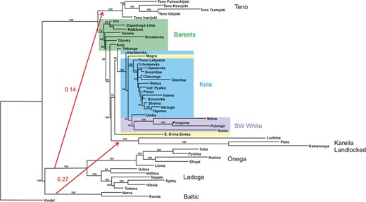
Results of the TreeMix analysis. Block colours show geographic regional groupings as in Figures 1 and 2. Numbers indicate nodal support based on 100 bootstrap trees without migration. Red arrows show long‐distance gene flow events inferred by TreeMix, with numbers indicating migration weight. The tree is unrooted
Genomic signatures of local selection within regional population groups
Three hundred and five SNPs were retained as ‘Outlier SNPs’ in the Barents analysis, 318 in the Kola analysis and 201 in the Teno re‐analysis (Table S3). These SNPs occurred within 263 independent haploblocks in Barents, 184 haploblocks in Kola and 80 haploblocks in Teno (Table S3). Only four of these outlying haploblocks were shared between all three regional groups, whereas a further 13 were shared between two groups (Table 2, Figure S3). In 10 of these 13 haploblocks, one or more Outlier SNPs were also shared between regional groups (Table 2); the other three shared haploblocks were labelled by different Outlier SNPs in the different groups. When examining the association between genomic variation and upstream catchment area, far fewer SNPs were retained as ‘GEA SNPs’: 20 SNPs in Barents, within 17 haploblocks; 14 SNPs in Kola, within13 haploblocks; and 123 SNPs in Teno, within 48 haploblocks (Table S3). Only a single catchment‐associated haploblock was shared between regional groups; this haploblock, on chromosome Ssa11, was also a shared outlier (Table 2, Figure S3).
Haploblocks containing candidate locally selected SNPs that were identified in more than one regional population group. Candidate SNPs identified from combined outlier analyses (‘Outlier SNPs’) or associations with upstream catchment area (‘GEA SNPs’)
| Outlier SNPs | GEA SNPs | Chr | HB_Start | HB_End | # shared candidate SNPs | Annotation |
| Barents, Kola | na | Ssa03 | 8,923,406 | 9,051,536 | 1/19 | ralyl, gimap8 |
| Barents, Kola | na | Ssa09 | 18,808,558 | 18,882,390 | 0/19 | cd276, kiaa1522, rbbp4, zbtb8os |
| Barents, Kola, Teno | Teno | Ssa09 | 24,572,313 | 24,956,797 | 28/55 | fgfrl1, tacc3, kif15, rd3, tdrd9, rtn1, lrrc9, pcnxl4, dhrs7, ppm1a, six6, pgbd4, six1 |
| Barents, Kola | na | Ssa09 | 70,676,323 | 70,691,232 | 1/1 | ppargc1b |
| Kola, Teno | na | Ssa10 | 19,245,658 | 19,414,999 | 0/25 | polrmt, fgf10, mcpt, cfd |
| Kola, Teno | Kola, Teno | Ssa11 | 19,198,258 | 19,305,775 | 2/9 | numa1, zfhx3, |
| Barents, Kola | na | Ssa12 | 25,150,145 | 25,570,229 | 1/23 | apoh, prkca, cacng5, |
| Barents, Kola | na | Ssa12 | 60,985,380 | 61,035,597 | 1/6 | slc41a1, etnk1, sox13 |
| Barents, Kola, Teno | na | Ssa12 | 61,472,809 | 61,699,297 | 6/45 | mdfi, tmem183a, ppfia1, tfeb, mhcII‐dab, |
| Kola, Teno | na | Ssa12 | 61,735,215 | 61,901,187 | 0/8 | perk8, foxp4 |
| Barents, Kola | na | Ssa13 | 71,035,682 | 72,586,328 | 0/52 | dlc1, sgcg, mrpl22, gemin5, cnot8, fam114a2, mfap3, glnt10, cdhrs11, ine, flot2a, tbx6l, eral, fam222b |
| Barents, Kola | na | Ssa18 | 58,936,002 | 58,952,501 | 1/2 | mfa3l |
| Barents, Kola | na | Ssa20 | 3,321,666 | 3,367,040 | 1/12 | suds3 |
| Barents, Kola, Teno | na | Ssa20 | 45,834,673 | 46,328,021 | 1/69 | ahnak, hipk4, pld3, fkh, irf2bp1, rpa34, nova1, gpr4, eml1, gcgr, cyp2m1, clip3, LOC106580757, akap12, tmem87b |
| Barents, Kola | na | Ssa21 | 320,945 | 642,361 | 0/17 | mycbp2, fbxl3, cln5 |
| Barents, Kola | na | Ssa21 | 12,187,008 | 12,190,232 | 0/21 | LOC106581842 |
| Barents, Kola, Teno | na | Ssa25 | 28,639,461 | 28,832,410 | 0/20 | vgll3, akap11, tnfsf11, epsti1, dnajc15 |
Chr: Chromosome; HB_Start, HB_end: start and end position of haploblock in bp; # shared candidate SNPs: how many SNPs in the haploblock were classed as candidate SNPs in two or more regional groups, compared to total number of shared SNPs in the haploblock; Annotation: annotated protein‐coding genes overlapping the haploblock.
DISCUSSION
Here, we used an allelotyping approach in combination with a 220K SNP array to characterize the population structure of Atlantic salmon in north‐eastern Europe, and ask whether the same loci emerge as locally adaptive candidates in independent analyses of different geographic regions. Our results largely recapitulated phylogeographic patterns that were previously inferred from much smaller marker sets. Although most candidate loci were unique to a single geographic region, several genomic segments repeatedly showed strong evidence for differential local selection across all three regions. The results from this study validate allelotyping as a reliable and cost‐effective alternative to individual genotyping when SNP genotyping arrays are available and the underlying population genetic structure is known.
Genome‐wide SNPs recapitulate population structure inferred from other markers
Analysis of genome‐wide SNP allele frequencies reiterated the population genetic structure found in earlier studies of the Atlantic salmon of north‐eastern Europe using microsatellites (Tonteri et al., 2005, 2009) and mtDNA (Asplund et al., 2004). We observed a clear genetic transition between the Barents and White Seas, with White Sea populations (Kola, E White Sea & SW White Sea) being distinct from Barents populations in the PCA and forming a well‐supported clade in the TreeMix analysis. This White Sea cluster was distant from the similarly well‐supported Baltic/Onega/Ladoga clade, with no inference of gene flow between the two: thus, our results do not support previous hypotheses of a close phylogeographic connection between the White Sea and the Baltic Sea (Kazakov & Titov, 1991; Makhrov et al., 2005). We observed further genetic differentiation between Kola Peninsula White Sea populations and E & SW White Sea populations. The SW White Sea populations in particular were strongly differentiated from one other and exhibited relatively low heterozygosity, suggesting that the observed structure in this region has been driven by population isolation and strong drift.
Our results are consistent with ancestral allopatry of Atlantic salmon in the Barents and White Seas, with subsequent gene flow between the two population clusters. In such a situation of secondary contact, genomic segments with elevated differentiation between the clusters may contain loci that are resistant to gene flow because they confer locally adaptive traits or otherwise reduce hybrid fitness (Wu, 2001). This pattern, however, can also emerge via other population genetic processes including linked purifying selection in areas of reduced recombination such as inversions (Cruickshank & Hahn, 2014; Lotterhos, 2019). Our analysis found segments of elevated differentiation between the Barents and Kola clusters to be distributed across 26 of the 29 chromosomes, with only a small number co‐occurring with known inversions (Table S2). Further investigation of possible genomic barriers to gene flow between the Barents Sea and White Sea Atlantic salmon lineages could improve our understanding of their recent evolutionary history and inform their management.
Strong candidates for differential local selection repeatedly emerge in replicated analyses
When analysing the Barents, Kola and Teno data sets independently, we identified numerous haploblocks that were unusually differentiated among populations within each region and so potentially harboured locally adaptative loci. Only four of these outlying haploblocks, however, were shared between all three geographic regions. For three of these four haploblocks (on chromosomes Ssa09, Ssa12 and Ssa25), there is powerful additional evidence for the presence of a selective target. This includes observations of locally extended haplotype homozygosity in the previous Teno River analysis (Pritchard et al., 2018) and well‐documented genotype–phenotype associations. The Ssa25 haploblock encompasses vgll3‐akap11, a large‐effect locus that strongly influences age at sexual maturity throughout the European range of Atlantic salmon and probably further afield (Ayllon et al., 2015; Barson et al., 2015; Kusche et al., 2017). Age, and therefore size, at sexual maturity is expected to have varying effects on fitness depending upon the physical and biological environment a salmon encounters during return spawning run; thus, differential selection among rivers is expected. Correspondingly, the age‐at‐maturity distribution of males and females varies substantially among the rivers included in this study (Primmer et al., 2006; Vähä et al., 2007). The haploblock encompassing six6, on Ssa09, has emerged repeatedly as a candidate for differential local selection throughout the range of Atlantic salmon (Pritchard et al., 2018). Variation in this genomic segment correlates with both age at maturity and seasonal timing of the return spawning migration (Barson et al., 2015; Cauwelier et al., 2017; Pritchard et al., 2018). Major histocompatibility complex II, on the Ssa12 haploblock, is well known for its role in pathogen response. For example, in Atlantic salmon, genetic variation at this MHCII‐containing segment is implicated in resistance to piscine myocarditis virus (Hillestad et al., 2020). Although much previous work on MHCII has focused on maintenance of genetic variability by balancing selection, there is strong evidence of differential local selection on MHCII genotype in other salmonid species (Larson et al., 2014, 2019; McClelland et al., 2013).
In the Teno River, Pritchard et al. (2018) found a correlation between vgll3 and six6 allele frequencies and upstream catchment area, a surrogate for river flow volume. This association was not observed in Barents or Kola, and over all we found rather few environmentally associated haploblocks when analysing the allelotyped data. This may be due to the unbalanced nature of the Barents and Kola data sets, which contained many rivers with small catchment areas and a few with very large ones (Table 1). Only one genomic tract, on chromosome Ssa11, was associated with upstream catchment area in more than one regional group; this haploblock, containing the genes numa1 and zfhx3, was also a shared outlier. It has been observed to co‐vary with seasonal migration timing in the Teno (Pritchard et al., 2018), and is unusually differentiated between populations of Atlantic salmon in northern and southern Norway (Kjærner‐Semb et al., 2016).
Our results are likely to underestimate the true overlap between locally selected targets among the three different regional groups of populations that we examined. The identification of outliers by combining evidence from several different statistical approaches is expected to be biased towards loci that show the strongest signals of selection within the Barents, Kola or Teno data sets (Forester et al., 2018). We also expect variation among data sets in the power we have to identify outliers due to the different number of populations examined, and the presence of many SNP markers linked to a single candidate locus which reduces the number of markers available to label other candidate loci when a fixed‐rank cut‐off for selection is applied. Additionally, in contrast to whole‐genome sequence data, the average density of SNPs on the array (~1 SNP per 15 kb) is unlikely to provide sufficient coverage of all possible selected variants. Further, in some cases, strong selection may have driven a variant to fixation in one of the geographic areas. For example, in Barents and Kola, we observe particularly strong evidence for differential local selection at a segment 18.8 Mb along chromosome Ssa09 (Table 2). This locus, which closely flanks a genomic segment recently implicated in adaptation to a landlocked life history (Kjærner‐Semb et al., 2020), is barely variable within the Teno populations analysed. We note, however, that the vast majority of identified ‘candidate loci’, including those previously inferred in the Teno River study of Pritchard et al. (2018), are unique to one of the three independent analyses. We suggest that this reflects a combination of false positives and truly different genomic architecture of local adaptation among regions.
Our results add to the growing evidence that adaptive diversification does not only occur by polygenic changes but can also involve large phenotypic shifts driven by single genes (or tightly linked genetic clusters). Such large‐effect loci, previously considered unlikely to contribute to complex locally adaptive traits, now been identified in a wide range of taxa (reviewed in Oomen et al., 2020). Here, we have identified several genomic segments with evidence for strong differential local selection among neighbouring populations of salmon across a wide area of northern Europe, including two phylogeographically distinct lineages. Several of these segments have previously been identified as selective targets across the broader Atlantic salmon distribution (Pritchard et al., 2018) and even in other salmonid taxa (Larson et al., 2019; Pritchard et al., 2018; Veale & Russello, 2017). Although the expectation remains that most local adaptation is polygenic, an influence of large‐effect loci can greatly alter evolutionary dynamics (Oomen et al., 2020). These strongly selected loci in Atlantic salmon are ideal targets for experimental validation of their role in local adaptation by characterizing their phenotypic consequences and examining their influence on fitness in different environments.
ACKNOWLEDGMENTS
We would like to thank Jan Nilsson, Jaakko Erkinaro, Anti Vasemägi, and others who participated in samples collection. We are deeply grateful to Anni Tonteri and Mikhail Ozerov for extracting DNA for some of the samples more than 10 years ago. Special thanks to the reviewers for useful comments that improved the manuscript. This research has been funded by the Academy of Finland (grants 284941, 314254 and 327255). We are grateful to Sigbjørn Lien, Matthew Kent, and Silje Karoliussen for assistance with SNP allelotyping. The authors dedicate this work to the memory of our dear friend and colleague, Alexey E Veselov, who passed away on 03.05.2020.
CONFLICT OF INTEREST
The authors have no conflict of interest to declare.
AUTHOR CONTRIBUTIONS
CRP, VLP and KJZ conceived and designed the experiments. KJZ performed the experiments. VLP and KJZ analysed the data. AEV, JL and CRP contributed reagents/materials/analysis tools. KJZ and VLP wrote the paper, CRP, JL, and AEV commented on the manuscript.
Peer Review
The peer review history for this article is available at https://publons.com/publon/10.1111/jeb.13732
DATA AVAILABILITY STATEMENT
Raw data and code used in the analyses are archived in Dryad Digital Repository: https://doi.org/10.5061/dryad.sn02v6x2t
REFERENCES
Author notes
The authors dedicate this work to the memory of our dear friend and colleague, Alexey E Veselov, who passed away on 03.05.2020.
