


Abstract
Optimal camouflage can, in principle, be relatively easily achieved in simple, homogeneous, environments where backgrounds always have the same colour, brightness and patterning. Natural environments are, however, rarely homogenous, and species often find themselves viewed against varied backgrounds where the task of concealment is more challenging. One result of variable backgrounds is the evolution of intraspecific phenotypic variation which may either be generalized, with multiple similarly cryptic patterns, or specialized, with each discrete colour form maximizing concealment against a single component of the background. We investigated the role of phenotypic variation in a highly variable population of the Neotropical toad Rhinella margaritifera using visual modelling and a computer‐based detection task. We found that phenotypic variation was not divided into discrete colour morphs, and all toads were well camouflaged against the forest floor. However, although the whole population may appear to consist of random samples from the background, the toads were a particularly close match to the leaf litter, suggesting that they masquerade as dead leaves, which are themselves variable. Furthermore, rather than each colour form being equally effective against a single background, each toad was specialized towards its own particular local surroundings, as suggested by a specialist strategy. Taken together, these data highlight the importance of background matching to a nominally masquerading species, as well as how habitat heterogeneity at multiple spatial scales may affect the evolution of camouflage and phenotypic variation.
Abstract

INTRODUCTION
Camouflage is a well‐known and widespread adaptation that protects animals from detection and/or recognition (Cuthill, 2019; Stevens & Merilaita, 2009a). Visually guided predators make use of multiple visual cues to segment their prey from the background, and so effective concealment can take many different forms (Cuthill et al., 2017; Troscianko et al., 2009). As such, camouflage patterns may utilize colour, intensity, spatial frequency, or the orientation of pattern to either match the background or disguise recognizable features (Cuthill, 2019; Endler, 1981; Stevens & Merilaita, 2009a). Moreover, the characteristics of the background itself, including colour and pattern heterogeneity as well as larger spatial structure, will affect the efficacy of visual search tasks and therefore influence the evolution of camouflage (Barnett et al., 2016; Dimitrova & Merilaita, 2009; Endler, 1984; Kjernsmo & Merilaita, 2012; Merilaita, 2003; Michalis et al., 2017; Xiao & Cuthill, 2016). In this paper, we quantify colouration in a highly variable Neotropical toad, Rhinella margaritifera (Bufonidae; Laurenti, 1768) and relate this to variation in the local microhabitat.
Although there are many forms of camouflage, three categories are arguably the most widespread and well characterized: preventing detection through background matching or disruption and preventing recognition through masquerade (Cuthill, 2019; Stevens & Merilaita, 2009a). Background matching, perhaps the most intuitive form of camouflage, reproduces environmental colours and patterns to minimize the signal‐to‐noise ratio between a target and its background (Merilaita et al., 2017). Disruptive camouflage breaks up the outline, or surface, of a target with high contrast patterns that differentially blend into the background (Cott, 1940; Merilaita et al., 2017; Stevens & Merilaita, 2009b). Masquerade, on the other hand, disrupts recognition rather than detection, with species mimicking whole background features, such that even if a target is perceptually segmented from the background, it may still be dismissed as an inedible or irrelevant object (Skelhorn et al., 2010; Skelhorn et al., 2010).
Although background matching may at first appear simple, it does have an important limitation. As the number of possible colours and patterns in an environment increases, the likelihood that a single pattern will closely match its immediate surroundings decreases (Michalis et al., 2017). The evolutionary response to a highly variable background largely follows two distinct routes: (a) to produce a generalist pattern which trades off the degree of matching within each patch for an acceptable level of camouflage across multiple locations, or (b) to specialize for high‐fidelity camouflage within a certain subsection of the background at the cost of camouflage in other areas (Houston et al., 2007; Hughes et al., 2019; Merilaita et al., 1999, 2001). The evolution of generalist or specialist strategies can be broadly linked to the spatial scale of background heterogeneity, where variation over an area smaller than the target favours generalist camouflage and variation on a scale larger than the target leads to specialist strategies (Bond & Kamil, 2002, 2006).
Furthermore, the evolutionary processes leading to generalist or specialist camouflage can also play out within species. This frequently results in phenotypic variation, which may be apparent as discrete morphs or as continuous variation, and may be found within populations of sympatric individuals or in allopatry (Rojas, 2017). Bond (2007) defined two categories of sympatric polymorphism: generalist polymorphism and specialist polymorphism. Generalist polymorphism evolves in fine‐grained, visually complex, environments where a species may diversify into a large number of sympatric colour forms with similar efficacy. Each colour form acts as generalist camouflage and matches a subsample of the visual characteristics of the background (Bond, 2007; Bond & Kamil, 2006). In contrast, in coarse‐grain, spatially structured, environments specialist polymorphism is more likely to evolve. Here, each colour form evolves towards maximum concealment against the particular local features of its own microhabitat, although each is less effective outside its local patch (Bond, 2007; Karpestam et al., 2013). However, despite these predictions research into naturally occurring colour patterns has primarily focused on the evolution of discrete polymorphism in allopatric populations, with comparatively little attention paid to continuous variation found within populations.
Here, we investigate whether sympatric continuous variation in the camouflage patterns of R. margaritifera conforms to the predictions of generalist or specialist camouflage strategies, and whether variation has detectable effects on camouflage efficacy. These toads are sit‐and‐wait predators that live amongst the rainforest leaf litter where their highly variable colour patterns appear to be well camouflaged (McElroy, 2016) (Figure 1). However, although R. margaritifera is highly toxic (Sinhorin et al., 2020), the toads do appear to be at risk from predators including birds, snakes and mammals (Gompper, 1996; Kollarits et al., 2013; McElroy, 2016; Oliveira et al., 2017; Toledo et al., 2007). Indeed, as the toads’ diet primarily consists of invertebrates, a large proportion of which are ants, it seems unlikely that high‐fidelity camouflage would evolve to aid in prey capture although the same principles of camouflage evolution would still apply (Almeida et al., 2019; Pembury Smith & Ruxton, 2020).
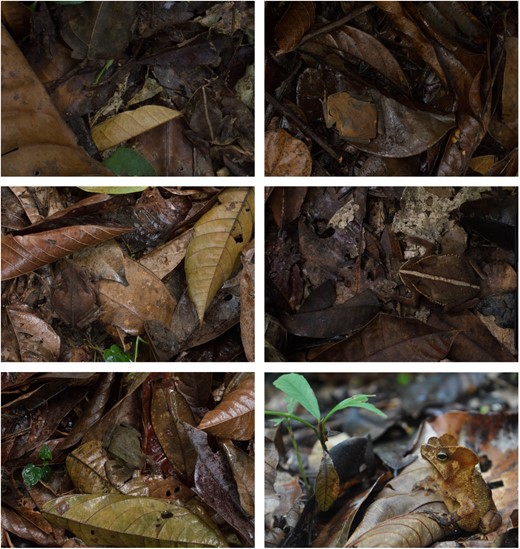
Examples of variation in toad colouration and local background characteristics
To investigate the efficacy of toad camouflage, we first used image analysis and visual modelling to assess whether toad variation falls into discrete colour morphs, as well as how well toads matched different components of the background. Then, to examine whether phenotypic variation was targeted toward local background characteristics (spatial microhabitat specialization), we ran a computer‐based detection experiment with human participants in which we presented toads on backgrounds from either near to where they were found, or randomly drawn from the wider environment. If the toads are utilizing a specialist strategy, we would expect to find discrete colour forms and that each morph was less detectable in patches near to where they were found. Conversely, if the toads use a generalist strategy, variation may be continuous or discrete, but detectability would be expected to be equal across the whole visual environment.
MATERIALS AND METHODS
Study species
The R. margaritifera species complex extends throughout tropical northern South America and into Central America. Currently, ~20 species have been described within the complex; however, the group systematics are complicated, with the geographic, genetic and phenotypic boundaries between species being difficult to discern (Fouquet et al., 2007; Lavilla et al., 2013; Pereyra et al., 2021).
At La Station de Recherche en Écologie des Nouragues (Nouragues Natural Reserve, French Guiana), there are three morphologically distinct clades of the R. margaritifera complex: R. castaneotica, R. lescurei and R. c.f. margaritifera. We focused on phenotypically identified R. c.f. margaritifera (hereafter R. margaritifera) which are distinct from R. castaneotica and R. lescurei due to the presence of a bony knob in the corner of the mouth and a row of tubercles running from the parotoid gland to the groin (Avila‐Pires et al., 2010; Hoogmoed, 1986), as well as larger size, the presence of large bony cranial crests and, in the female, dorsal vertebral spines (Avila‐Pires et al., 2010; Fouquet et al., 2007; Fouquet et al., 2007).
Image collection
We searched for adult R. margaritifera along 10 independent transects through the rainforest at La Station de Recherche en Écologie des Nouragues (Barnett et al., 2018b) (Figure 1). The transects were ~250 m in length and were separated by ~20 m with direction alternating either side of the central path. We photographed the dorsal pattern of each toad (n = 62), as well as the natural leaf litter background from within 1 m of 52 of the toads (local background: n = 4 non‐overlapping images per toad) and at ~5 m intervals along each transect (wider environment: n = 500, 50 per transect). Toads and backgrounds were photographed from heights of 70 cm and 150 cm, respectively (each background image covered ~80 cm × ~50 cm of the forest floor), with a Nikon D3200 DSLR camera and AF‐S DX NIKKOR 35 mm prime lens (Nikon Corporation, Tokyo, Japan), and all images contained a ColorChecker Passport (X‐Rite Inc., Grand Rapids, MI, USA). Each image was converted to a 300 dpi, 8‐bit, TIFF file, and the ColorChecker was used to scale, linearize and colour calibrate the image (Stevens et al., 2007) in MATLAB 2017a (The MathWorks Inc., Natick, MA, USA).
Image analysis—visual modelling
The visual modelling followed that outlined in previous work (Barnett et al., 2017, 2018a, 2018b, 2020; Xiao & Cuthill, 2016). We used the peak wavelength sensitivity values (λmax) from the cone cells of three ecologically relevant predators (Gompper, 1996; Kollarits et al., 2013; McElroy, 2016; Oliveira et al., 2017; Toledo et al., 2007): tetrachromatic birds (Hart, 2002; Toledo et al., 2007; Willink et al., 2014), trichromatic snakes (Kollarits et al., 2013; Macedonia et al., 2009) and dichromatic mammals (Calderone & Jacobs, 2003; Gompper, 1996; Jacobs & Deegan, 1992). The bird model used the violet‐sensitive tetrachromatic vision of the Indian peafowl (Pavo cristatus: λmax LWS = 605, MWS = 537, SWS = 477, VS = 432 nm, and D = 567 nm (Hart, 2002)), the snake model used the trichromatic vision of the coachwhip (Masticophis flagellum: λmax LWS = 561, MWS = 458 and UV = 362 nm (Macedonia et al., 2009)), and the mammalian model used the dichromatic vision of the domestic ferret (Mustela putorius: λmax LWS = 558 and SWS = 430 nm (Calderone & Jacobs, 2003)). We also included human L*a*b* colour space to allow for more intuitive interpretation of the data (CIELAB, 1976). We used natural daylight (D65); however, as there is minimal UV reflectance from the toads (McElroy, 2016) and minimal UV irradiance below the canopy (Théry, 2001), we did not include UV in our analysis.
Each visual model comprised a measure of achromatic intensity, henceforth luminance (L) and two opponent channels of hue (red‐green (rg) and yellow‐blue (yb)) which were analogous to the L*a*b* channels developed through behavioural testing of human visual perception (hereafter luminance and hue together are referred to as ‘colour’). Analysis of patterning followed Michalis et al. (2017), with pattern information being extracted using a log‐Gabor filter bank in MATLAB 2017a. These filters produced 24 dimensions, resulting from four spatial frequencies (wavelengths relative to the width of the smallest toad: very high = ⅛, high = ¼, medium = ½ and low resolution = 1), and six orientations (0°–150° in 30° increments) convolved with the luminance channel of each image (Barnett et al., 2018a, 2018b; Field, 1987; Gabor, 1946). As the background was isotropic, with no preferred direction, we reduced the number of dimensions by selecting the orientation with the maximum spectral energy for each spatial frequency. This produced three dimensions of colour (L, rg and yb) and four of pattern (very high, high, medium and low spatial frequencies).
Image analysis—polymorphism
As toad colouration was variable, we explored whether the toads fell into discrete morphs using factor analysis and k means clustering in R 3.6.1 (R Core Team, 2019). For each visual model, we calculated the mean of each of the three colour channels (L, rg and yb) and the mean of each pattern channel (very high, high, medium and low) from each toad. Toad colour varied from dark red brown to light beige, and pattern variation included homogeneous colours, small speckles, large irregular blotches and a mediodorsal stripe that varied in both intensity and width (Figure 1). Each of these pattern components would be identifiable by the characteristic distribution of mean energy across spatial frequency channels. In the factor analysis (R function factanal), we used varimax rotation and three factor classes for each visual model. In the k means clustering, we assessed the optimal number of clusters between one and 10, using the ‘elbow’ method and through silhouette analysis (R package cluster (Maechler et al., 2019); R function kmeans; Figure 2). The ‘elbow’ method identifies the point at which additional clusters begin to offer diminishing returns in explaining variance within a dataset. The silhouette coefficient is a measure of variance within clusters compared to that between clusters, with higher values indicating a more efficient number of groupings. All subsequent analyses used the raw dataset rather than the means or factor scores.
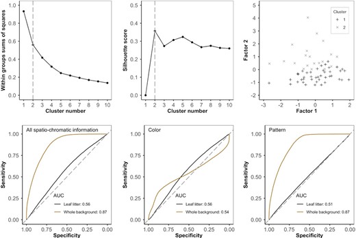
Image analysis using the avian visual model. Top: Plotting the within‐groups sums of squares (left) and the silhouette score (centre) for cluster numbers 1 to 10 shows that two clusters are the most suitable. However, plotting these two clusters along the two main factor axes (right) shows that there is no discrete boundary between clusters and toad variation is continuous. Bottom: ROC curves with the area under the curve (AUC) representing the accuracy with which the avian visual model could discriminate between toads and the two backgrounds (leaf litter and whole background). With all spatio‐chromatic information (left), toads are a closer match to the leaf litter than to the background as a whole. Analysing colour (centre) and pattern (right) separately shows that a mismatch in pattern between toads and the whole background underlies the difference in classification accuracy. AUC of ROC curves: 0.5–0.6 = fail, 0.6–0.7 = poor, 0.7–0.8 = fair, 0.8–0.9 = good and 0.9–1.0 = excellent
Image analysis—camouflage efficacy
To assess the efficacy of camouflage and to investigate what components of the background the toads matched most closely, we compared the accuracy with which a binary statistical classifier could discriminate between the toads and their backgrounds as viewed by the visual models. We used all 62 toads and randomly selected 124 background images from the wider environment. In order to assess whether the toads matched the background or masqueraded as dead leaves, we selected the whole background from 62 of the background images and selected only the leaf litter (without soil, stones, shadows, or new plant growth) from the other 62 background photographs. One thousand pixels were then selected using MATLAB’s uniform random number generator, without replacement, from each toad and from each background (Barnett et al., 2018a, 2018b, 2020).
We first assessed camouflage efficacy using all spatio‐chromatic data (colour = L, rg, yb; pattern: very high, high, medium, low), but then we analysed colour and pattern separately to discern what aspects of the background the toads matched most effectively. Discrimination accuracy was assessed with a binomial generalized linear mixed effects model (R package lme4 (Bates et al., 2015)) in R 3.6.1. Each channel from the visual model was centred and scaled (R function scale) and, to avoid overfitting the models, we used twofold cross‐validation where the toads were randomly split into two groups, with one used to train and the other to test the model (Barnett et al., 2018a, 2018b, 2020; Lantz, 2013). Classification accuracy was assessed using the area under the curve (AUC) of receiver operating characteristic (ROC) curves (Lantz, 2013) (R package pROC (Robin et al., 2011)). The AUC represents the probability of correct identification, with an AUC of 0.5 no better than allocating objects by chance and 1.0 indicating perfect discrimination of object type. We followed a common grading system, interpreting AUC as: 0.5–0.6 = fail, 0.6–0.7 = poor, 0.7–0.8 = fair, 0.8–0.9 = good and 0.9–1.0 = excellent (Barnett et al., 2018a, 2018b, 2020; Lantz, 2013).
Detection—local camouflage
To assess whether camouflage was most effective at the site where the toad was first encountered, we ran a screen‐based detection experiment with human ‘predators’. Human visual perception does differ from that of the toads’ natural predators, and care should be taken when using humans as surrogate predators. However, when directly compared humans and birds have been repeatedly found to have similar responses to camouflaged targets in the absence of UV reflectance (Barnett et al., 2016, 2018a, 2018b, 2020; Kjernsmo et al., 2020; Olsson et al., 2015; Troscianko et al., 2009; Xiao & Cuthill, 2016). Participants (n = 30), with normal or corrected‐to‐normal vision, were tasked with finding and mouse‐clicking on the toads presented against their local backgrounds and against randomly selected backgrounds from the wider environment. All participants gave their informed consent in accordance with the Declaration of Helsinki, and the experiments were approved by the University of Bristol Faculty of Science Research Ethics Committee.
We used the calibrated photographs of the 52 toads for which we had photographs of the local forest floor. For each toad, we randomly selected two calibrated photographs of its local environment and cropped a square region of interest (ROI) from each to act as the local background condition. For the random background condition, we randomly selected 52 images from the wider environment and from each we selected two independent ROIs of the background. This ensured that each condition captured a similar area of the forest floor and controlled for any differences in background variance. Each toad was then combined with the two local ROIs and two randomly selected random ROIs to create 208 toad–background combinations. The toads were cropped from their photographs and pasted onto the background images with both location (x‐y coordinates) and orientation (integer rotation between 0° and 359°) randomly selected from a discrete uniform distribution generated in MATLAB 2017a.
Prior to data collection, participants were briefed on the experimental procedure and presented with six training images in which the toad's location was identified. Each participant was then presented with an independently randomized sequence of the 208 stimuli split into four blocks of 52 images. Participants were free to take a break between blocks, but, in practice, none paused for more than a few seconds. We recorded the time taken to click on the toad (response time) for all events where the mouse‐click was located within the outline of the toad. Stimuli where the mouse‐click was outside the toad, or if there was no mouse‐click within 35 s, were recorded as missed. The 35 s time‐out criterion was chosen to be sufficient for the toad to be found in most trials, based on pilot runs by the authors.
The experiment was run in MATLAB 2017a using the Psychtoolbox extensions (Brainard, 1997) on a gamma‐corrected Iiyama Vision Master Pro 513 monitor (Iiyama Corp., Tokyo, Japan) connected to a MacBook Pro laptop (Apple Inc., Cupertino, CA, USA). Log‐transformed response time (only for trials where the target was detected) was analysed with a linear mixed effects model, and the number of correct and incorrect detections (detection accuracy) was analysed with a binomial generalized linear mixed effects model (R package lme4 (Bates et al., 2015)) in R 3.6.1. Both models included treatment (local or random background) as a fixed effect, and the identification numbers of the toad, the background and the participant were included as random factors.
RESULTS
Visual modelling—polymorphism
Using the avian visual model, factor analysis identified three main dimensions in the data (cumulative variance explained = 78.8%): 1—the intensity of the dorsal stripe (28.6% variance), 2— toad colour ranging from light brown to dark red (26.9% variance), and 3—the presence of low spatial frequency blotches (23.3% variance). In the k means clustering, silhouette analysis indicated that the optimal number of clusters was two (covering 40.0% variance). However, when plotting cluster values against factors 1 and 2, we found there to be no distinct boundaries between clusters (Figure 2). We therefore found no evidence to suggest that variation in toad colouring is divided into discrete morphs; instead, variation appears to be continuous. A similar trend was found in the computational models of snake, mammal and human vision (Table 1).
Percent variance explained through factor analysis and k‐means cluster analysis for each model of visual perception
| Variance explained (%) | Avian | Snake | Mammal | Human |
| Factor analysis | ||||
| Factor 1 | 28.6 | 28.7 | 31.5 | 26.3 |
| Factor 2 | 26.9 | 27.1 | 29.3 | 25.3 |
| Factor 3 | 23.3 | 25.3 | 6.8 | 24.4 |
| Cumulative variance | 78.8 | 81.1 | 67.6 | 76.0 |
| k‐means clustering | ||||
| k = 2 | 40.0 | 62.2 | 52.6 | 52.4 |
Visual modelling—camouflage efficacy
When comparing colour and pattern between the toads and the background, we found that the toads were a better match to the leaf litter component of the background than to the background as a whole. When analysing colour and pattern information together (all spatio‐chromatic information), all visual models were good at discriminating toads from the whole background, but all models failed to discriminate the toads from the leaf litter. When considering colour information alone, all visual models failed to discriminate toads from both the leaf litter and the whole background. However, with pattern we found that all models were good at separating toads from the whole background, but each model failed to separate the toads from the leaf litter (Figure 2; Table 2).
Discrimination accuracy between toads and the two backgrounds for each visual model
| Area under the curve | Avian | Snake | Mammal | Human |
| All spatio‐chromatic information | ||||
| Leaf litter | 0.56 | 0.55 | 0.56 | 0.54 |
| Whole background | 0.87 | 0.87 | 0.86 | 0.86 |
| Colour | ||||
| Leaf litter | 0.56 | 0.55 | 0.55 | 0.54 |
| Whole background | 0.54 | 0.56 | 0.51 | 0.50 |
| Pattern | ||||
| Leaf litter | 0.51 | 0.51 | 0.51 | 0.51 |
| Whole background | 0.87 | 0.87 | 0.87 | 0.87 |
Area under the curve (AUC) of ROC curves: 0.5–0.6 = fail, 0.6–0.7 = poor, 0.7–0.8 = fair, 0.8–0.9 = good and 0.9–1.0 = excellent.
Detection—local camouflage
Human participants took significantly longer to find toads against their local, as opposed to random, backgrounds (χ2 = 6.00, df = 1, p = 0.014; Figure 3 top‐right). There was, however, no statistically significant difference in detection accuracy, the trend being towards more detection errors on local backgrounds; this indicates that the response time data were not subject to a speed–accuracy trade‐off (χ2 = 3.18, df = 1, p = 0.074; Figure 3 bottom‐right).
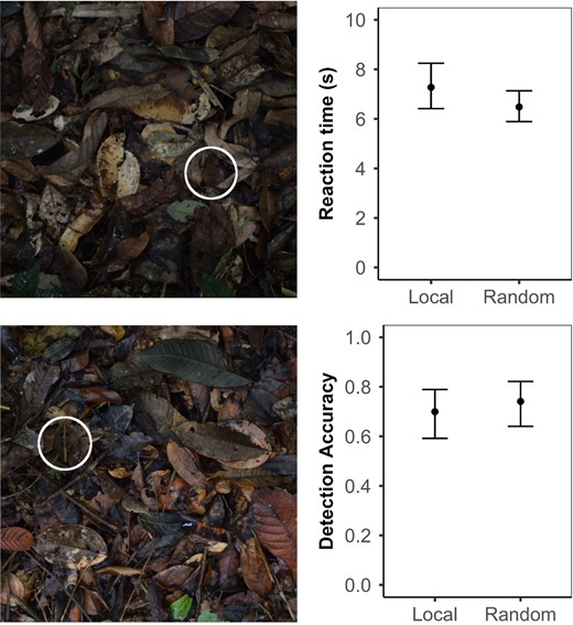
Detection experiment with human participants. Left: Example stimuli showing toads against the leaf litter background. Right: Local vs. random background detection experiment for toads presented on their local background vs a randomly selected background (means ± 95% CI from the model). Top‐right: response time, human participants took significantly longer to find toads on their local leaf litter than on randomly selected backgrounds. Bottom‐right: detection accuracy, there was no significant difference in detection accuracy between backgrounds
DISCUSSION
We found Rhinella margaritifera to be very well camouflaged against the forest floor, but, rather than specializing towards a single generalized background matching pattern, the toads were variable in both colour and patterning. The toads’ natural background is predominantly made up of a mix of fallen leaves, but also includes bare ground, fallen sticks, rocks, fungal fruiting bodies and new plant growth. Although toad colour was a good match across the whole background, toad patterning was only a close match to the leaf litter component. This close match in both colour and pattern between the toads and the leaf litter suggests that the toads masquerade as dead leaves. This conclusion was consistent between the different visual systems of avian, snake and mammalian predators.
Moreover, although the leaf litter may at first appear to be randomly distributed, and homogeneous over large scales, the visual environment does vary spatially depending on the composition of the overhead vegetation, the light environment and the moisture content found in the substrate. When this local variation was taken into account, we found that phenotypic variation resulted in toads being more difficult to detect within their own local patches. This effect was significant, but, as the absolute change in response time was slight and as screen‐based experiments cannot replicate all aspects of the three‐dimensional environment, further research is needed to confirm the ecological relevance of this effect under natural conditions and with natural observers. That said, in the wild—where toads are more sparsely distributed—the visual search task is expected to be more challenging, and any differences will be amplified.
Masquerade is frequently defined as camouflage without background matching, as it acts to disrupt recognition rather than detection and can continue to function even when isolated from its natural context (Skelhorn et al., 2010; Skelhorn et al., 2010). This may then suggest that, although colour and patterning would be tightly bound to those found within particular cohesive features (in this case dead leaves), selection to match the immediate microhabitat would be relaxed relative to background matching camouflage. Contrary to this prediction, however, we found that individual toads more closely matched local conditions within the wider visual environment.
This spatial assortment of toad colouration suggests that phenotypic variation develops as a result of microhabitat‐specific selection pressures. This variation was not, however, structured into well‐defined and distinct patches, but rather across a background characterized by continuous omnidirectional gradients as different individual trees influence the forest floor around them. This lack of larger spatial organization is more akin to the characteristics of a single heterogeneous background rather than a network of discrete and independent patches. On such heterogeneous backgrounds, continuous variation in camouflage may arise and be maintained by apostatic selection and the disruption of observer search image formation (Bond, 2007; Bond & Kamil, 2002, 2006; Karpestam et al., 2014, 2016). Such processes may be enhanced by greater diversity in colouration, but these toads do not conform to common assumptions regarding the random spatial distribution, and equal efficacy, of each colour form within the single background (Bond, 2007). The toad's phenotypic variation therefore appears to produce aspects of both specialist and generalist strategies across a small geographic area within which toads are not necessarily physically restricted to the patch where they were encountered. As such, toads may be able to benefit from both high‐fidelity local background matching, and from being distinct from sympatric conspecifics. It is, however, unknown whether this local matching was the result of selective predation, behaviourally mediated site selection, plasticity in colour development, or active colour change (Stevens & Ruxton, 2019; Stevens et al., 2017), although the implications for predator foraging behaviour remain the same. Future research is needed to understand whether this is a toad‐ or predator‐driven pattern, and to reveal what environmental cues the toads and their predators may be using for site selection, colour change, or prey choice.
Here, we found evidence that toad colouration acts as both masquerade and background matching, with toad colouring being a close match to the background and toad patterning being tailored towards mimicking leaf structure. McElroy (2016) also investigated the function of these colour patterns by recording the rate of predation on clay models representative of the Central American toad Rhinella alata (a phenotypically similar species within the R. margaritifera complex). McElroy (2016) found that when presented on the natural background, patterned models had a higher survival rate than plain coloured models, even when the base colour did not match the substrate. It is notable that many of the toads bear a light stripe down the middle of their back, rather like the petiole of a leaf, and diamond‐shaped blotches, both of which vary in intensity across individuals, and may act as masquerade (dorsal stripe) or surface disruption (high‐contrast blotches). Our data suggest that these different patterns are not discrete morphs but vary continuously with many individuals exhibiting intermediate patterns.
In the early days of camouflage research, strategies were defined by the characteristics of the pattern itself, whereas the modern description of defensive colouration focuses on how a pattern disrupts the perceptual processes of the observer (Cuthill, 2019; Merilaita et al., 2017; Stevens & Merilaita, 2009a). The current mechanistic approach unifies camouflage strategies in a manner independent from the particular features of the pattern but can result in ambiguity at the boundaries between different forms of camouflage. For example, although it appears possible for disruptive camouflage to function with (some) colours not found in the immediate background (Schaefer & Stobbe, 2006), efficacy can be higher when utilizing features found within the naturally occurring distributions of hue, luminance and pattern (Fraser et al., 2007; Stevens et al., 2006). Similarly, although masquerade can be effective when background matching is not possible, masquerading organisms will frequently be found amongst their models (Skelhorn et al., 2010; Skelhorn et al., 2010). Indeed, predators are less likely to detect masquerading prey both when the abundance of models is high and when they have previously encountered the model (Skelhorn et al., 2011; Skelhorn & Ruxton, 2011). Consequently, masquerading species can rely on background matching until perceptually segmented from the background (Skelhorn et al., 2011; Skelhorn & Ruxton, 2010a). Close comparison between masquerader and model can, however, allow predators to see through the disguise (Skelhorn & Ruxton, 2010b), and this is a factor that may select for greater site‐specific mimic fidelity. As the background contains variation at multiple spatial scales, the dominant camouflage strategy identified appears to depend on the scale at which we characterize the visual environment.
Considering our data, we find a complex interaction between background matching, masquerade and disruptive camouflage. We find that when a heterogeneous background contains continuous variation, specialist camouflage does not necessarily require discrete polymorphism and that background matching can be an important component of masquerade. These data stress the importance of taking context and multiple spatial scales into consideration when trying to understand how defensive colouration evolves.
ACKNOWLEDGMENTS
We would like to thank David Gibson (University of Bristol) for the log‐Gabor filter (MATLAB) code, N. Simon Sanghera (University of Bristol), Eric Guerra‐Grenier (McGill University), all members of CamoLab (University of Bristol) for discussion and the staff at the Nouragues Natural Reserve, French Guiana, for support in the field. This work was supported by a University of Bristol postgraduate scholarship (to JBB); the Centre National de la Recherche Scientifique (ANR‐10‐LABX‐25‐01 to JBB, CM, NES‐S, & ICC); and a Le Fonds de recherche du Québec – Nature et Technologies postdoctoral fellowship (PBEEE–V2: 263478 to JBB).
CONFLICT OF INTEREST
The authors have no conflict of interest to declare.
AUTHOR CONTRIBUTIONS
The experiments were conceived by JBB, CM, NES‐S and ICC. JBB and CM collected the data in the field, CM performed the detection experiment, and JBB, CM and ICC implemented the image analysis. JBB wrote the first draft of the manuscript with subsequent input from all authors.
PEER REVIEW
The peer review history for this article is available at https://publons.com/publon/10.1111/jeb.13923.
DATA AVAILABILITY STATEMENT
Raw data can be downloaded from the Dryad Digital Repository (https://doi.org/10.5061/dryad.b2rbnzsbc).
REFERENCES
Author notes
James B. Barnett and Constantine Michalis are joint first author.
