


Abstract
The study of ecological niche evolution is fundamental for understanding how the environment influences species' geographical distributions and their adaptation to divergent environments. Here, we present a study of the ecological niche, demographic history and thermal performance (locomotor activity, developmental time and fertility/viability) of the temperate species Drosophila americana and its two chromosomal forms. Temperature is the environmental factor that contributes most to the species' and chromosomal forms' ecological niches, although precipitation is also important in the model of the southern populations. The past distribution model of the species predicts a drastic reduction in the suitable area for the distribution of the species during the last glacial maximum (LGM), suggesting a strong bottleneck. However, DNA analyses did not detect a bottleneck signature during the LGM. These contrasting results could indicate that D. americana niche preference evolves with environmental change, and thus, there is no evidence to support niche conservatism in this species. Thermal performance experiments show no difference in the locomotor activity across a temperature range of 15 to 38 °C between flies from the north and the south of its distribution. However, we found significant differences in developmental time and fertility/viability between the two chromosomal forms at the model's optimal temperatures for the two forms. However, results do not indicate that they perform better for the traits studied here in their respective optimal niche temperatures. This suggests that behaviour plays an important role in thermoregulation, supporting the capacity of this species to adapt to different climatic conditions across its latitudinal distribution.
Introduction
The geographical distributions of species, in particular those of ectotherms, are partially determined by environmental variables such as temperature (Cossins & Bowler, 1987). Thus, the geographical range of any given species will be suggestive of their physiological tolerance (Hutchinson, 1957), and organisms respond to different environmental conditions by adapting genetically or by adjusting their phenotype (phenotypic plasticity) (Angilletta, 2009). In drosophilids, species' distributions reflect their upper thermal tolerance and there is a strong phylogenetic inertia in heat tolerance (Kellermann et al., 2012b). This suggests that the distribution of species is more limited by the lineage to which they belong than by local adaptation capacity. This may be true at the macroevolutionary level if climatic niche preference was constant over time; however, many Drosophila species have been able to invade different climatic regions (Parsons, 1983), demonstrating a capacity to adapt to new environments. For example, van Heerwaarden & Sgro (2013) have shown that D. simulans has the ability to respond to selection pressure towards increased upper thermal limits. This species also shows a plastic response to the diverse local conditions it encounters across its distributional range, performing optimally at a wide range of temperatures (Austin & Moehring, 2013). Contrary to this plasticity, individuals of D. melanogaster show adaptive response to the local conditions and perform better when subject to their local environment (Trotta et al., 2006). Thus, closely related species exhibit different responses to environmental change. In any case, there is evidence for a complex interplay between plastic, behavioural responses and the adaptive capacity of species (Calabria et al., 2012; Castañeda et al., 2013).
The study of ecological niches (Hutchinson, 1957; Soberon & Nakamura, 2009; Sillero, 2011) can be used to understand the effect of environmental change on species' distributions. These methods have been successfully used to accurately model the present, past and future distributions of many species (e.g. Waltari et al., 2007; Cordellier & Pfenninger, 2009; Jakob et al., 2010; Sillero & Carretero, 2013). To predict the future and past species' distributions, the current niche model of the species is extrapolated into the past and future climate reconstructions. However, this method relies on the niche conservatism assumption that species retain their ancestral ecological niche preferences. Combining ecological niche modelling (ENM) with inferences on the demographic history and phylogeography of the species provides a test of the assumption of niche conservatism. Recent phylogenetic analyses of temperature and desiccation tolerance in Drosophila suggest that this group of organisms show a conservative response to climate change (Kellermann et al., 2012a,b), which could be taken as evidence for phylogenetic niche conservatism. On the other hand, these studies did not specifically test this hypothesis using ENM and phylogeographical analyses for any of the Drosophila species included.
Drosophila americana belongs to the D. virilis group and has an estimated age of 1–1.6 million years (my) (Morales‐Hojas et al., 2008, 2011). It is native to the USA, inhabiting the Central and Eastern regions from Texas‐Florida to Montana‐Maine. It comprises two chromosomal forms, the northern form (D. a. americana) being characterized by a fusion of the chromosomes X and 4, whereas the southern form (D. a. texana) has these chromosomes unfused. Despite this difference in karyotype between populations, there is no evidence for significant genetic differentiation or population structure within the species, except at the base of the X chromosome (Vieira et al., 2006; Morales‐Hojas et al., 2008; Fonseca et al., 2013). The frequency of this rearrangement declines towards the south, where it is almost absent (McAllister, 2002; McAllister et al., 2008). This clinal distribution of the frequency of the chromosomal fusion indicates that natural selection is favouring one rearrangement over the other along a latitudinal transect. However, the shallow gradient of the cline, indicating a gradual change in frequency of the fusion, also shows that the selective force is not very strong. Despite this evidence, the factor responsible for the maintenance of the rearrangement gradient is unknown. The frequency of the fusion has been correlated with minimum January temperatures (McAllister et al., 2008), but this does not necessarily imply a causative relationship.
The main goal of the work presented here was to understand how a temperate species of Drosophila responds to different environmental conditions across its distribution. For this, we have first established what environmental factors constitute the niche and determined the distribution of D. americana using ecological niche modelling. We have also investigated the differences in niche preference between strains from the south and the north of the distribution and their performances under different thermal conditions to understand whether they are differentially adapted to different local temperature regimes. We have also analysed the evolution of niche preference of the species by extrapolating the present species model to the last glacial maximum (LGM; ~21 000 years ago) and the last interglacial (LIG; ~120 000–140 000 years ago) conditions in combination with a demographic analysis using DNA sequences to test the niche conservatism hypothesis.
Materials and methods
Environmental niche modelling
We used correlative methods of ecological niche modelling (Guisan & Zimmermann, 2000) requiring georeferenced presence‐only data and GIS‐based environmental data. The location data for D. americana were obtained from our collection sites (available at http://evolution.ibmc.up.pt; see also Reis et al., 2008) and those made available by Bryant McAllister (http://www.biology.uiowa.edu/mcallister/bfm_flies.html) (Appendix S1; Fig. 1a,b). We used 19 climatic variables from the WorldClim series (Hijmans et al., 2005; www.worldclim.org/): BIO1 = Annual Mean Temperature; BIO2 = Mean Diurnal Range [Mean of monthly (max temp–min temp)]; BIO3 = Isothermality (BIO2/BIO7); BIO4 = Temperature Seasonality (standard deviation ×100); BIO5 = Max Temperature of Warmest Month; BIO6 = Min Temperature of Coldest Month; BIO7 = Temperature Annual Range (BIO5–BIO6); BIO8 = Mean Temperature of Wettest Quarter; BIO9 = Mean Temperature of Driest Quarter; BIO10 = Mean Temperature of Warmest Quarter; BIO11 = Mean Temperature of Coldest Quarter; BIO12 = Annual Precipitation; BIO13 = Precipitation of Wettest Month; BIO14 = Precipitation of Driest Month; BIO15 = Precipitation Seasonality (Coefficient of Variation); BIO16 = Precipitation of Wettest Quarter; BIO17 = Precipitation of Driest Quarter; BIO18 = Precipitation of Warmest Quarter, and; BIO19 = Precipitation of Coldest Quarter. The spatial resolution of the variables was 30 arc‐seconds (approximately 1 km2), except for the LGM variables, with 2.5 arc‐minutes (approximately 5 km2). We calculated a Pearson correlation test to remove the bioclimatic variables that were most correlated (Appendix S2). Seven showed correlation values equal or lower than 0.75 (after rounding to two decimal places) and were included in the analyses. Models using alternative variables related to minimum temperatures were also estimated. We used three past climate scenarios in the analyses: one for the last interglacial (LIG: ~120 000–140 000 years BP; Otto‐Bliesner et al., 2006) and two (CCSM and MIROC) for the last glacial maximum (LGM: ~21 000 years BP).
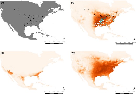
Presence data points (a) used to predict Drosophila americana's present distribution model (b). White squares represent locations of D. a. texana, black dots those of D. a. americana, and the triangles are the locations where heterozygotes have been observed. Drosophila americana distribution model predicted for the last glacial maximum (MIROC model) is depicted in (c) and the model for the last interglacial in (d).
We applied the maximum entropy (Maxent) method to estimate the following models of the realized ecological niche (sensu Sillero, 2011):
The model of the species in current climatic conditions of North America and projected to past climatic conditions.
The models of the two chromosomal forms in current climatic conditions. Populations were included in the americana or texana models when they showed ≥ 10% homozygous individuals for the fused or unfused X and 4 chromosomes, respectively (Appendix S1).
The models of D. americana and its chromosomal forms using current climatic conditions, with an alternative set of variables (removed from model 1, above) and related to minimum temperatures.
Models were estimated using the software maxent 3.3.3k (Phillips et al., 2004, 2006). This method is well suited to noisy or sparse information and is capable of dealing with continuous and categorical variables at the same time. Furthermore, it has been shown to outperform other methods, especially when samples sizes are low (Elith et al., 2006; Hernandez et al., 2006). We ran maxent with autofeatures (for establishing automatically the type of relationships among variables), randomly selecting 75% of the presence records as training data and 25% as test data. Ten model replicates were run. maxent then estimated the arithmetic mean with standard deviation of their projections through an iterative process (for a review on consensus models see Marmion et al., 2009). We tested the performance of maxent with receiver operated characteristics (ROC) plots. The area under the curve (AUC) of the ROC plot is a measure of the overall fit of the models (Liu et al., 2005). We selected AUC because it is independent of prevalence (the proportion of presence in relation to the total dataset size; VanDerWal et al., 2009), although recent critiques question the reliability of this measure (Lobo et al., 2008).
We used these models to identify the importance of each environmental variable for explaining the species' distribution by estimating: (i) the permutation importance determined by randomly changing the variable values among the training points and measuring the corresponding decrease in training AUC; thus, a model will depend strongly on those variables with a high decrease in permutation importance; (ii) jack‐knife analysis of the average AUC with training and test data; and (iii) average percentage contribution of each ecogeographical variable (EGV) to the models.
Additionally, we applied Ecological Niche Factor Analysis (ENFA, Hirzel et al., 2002) to the chromosomal forms of D. americana using the complete set of variables. ENFA models provide valuable ecological information about the realized niche of the species (Hirzel et al., 2002; Sillero et al., 2009; see below). ENFA was performed with biomapper 4.0 software (Division of Conservation Biology, University of Bern, Bern, http://www.unil.ch/biomapper). It compares the distributions of the environmental variables between the presence dataset (the species niche) and the whole study area, summarizing all the environmental variables into new uncorrelated factors with ecological meaning. Individual models, ranging from 0 to 100, were derived using the distance geometric mean algorithm (Hirzel & Arlettaz, 2003; Brotons et al., 2004). This algorithm makes no assumption on the shape of the species' distribution and takes into account the density of observation points in an environmental context by computing the geometric mean of all observation points. We evaluated ENFA models with an area‐adjusted frequency cross‐validation process (Boyce et al., 2002). The species locations were randomly partitioned into k different sets of equal size, k times. Each time, k‐1 partitions were used to compute the model, and the excluded partition was used for validation. Each model was reclassified into i bins, obtaining the area‐adjusted frequency for each bin as the proportion between the validation points (Ni) and the total area map (Ai): Fi = Ni/Ai. The expected Fi is 1.0 for all bins if the model is completely random. Low values of habitat suitability index should have a low F (below 1.0) and high values a high F (above 1.0). The predictive power of the model, measured by a Spearman rank correlation, was considered greatest when all Fi had a similar value (Boyce et al., 2002).
Samples and gene sequencing
The demographic history of the species was estimated using partial sequences from 16 genes in chromosomes 2 and 3 (Appendix S3). Polymorphic chromosomal inversions can confound the inference about the demographic history of the species, because the genetic signature reflects the evolutionary history of the rearrangement rather than that of the species. These chromosomes show no genetic structure across the species range (Morales‐Hojas et al., 2008) and are thus good candidates to study the demographic history of the species. Gene sequences for CG3223, CG9631, ebony, tll, pHCl and tra were available in GenBank (Table 1; Maside & Charlesworth, 2007; Morales‐Hojas et al., 2008, 2009). Genes geko, CG7255, sprk79D, dpr10, nkd, mub, CG8398, CG9674, CG14820 and Pk61C were recently obtained by the authors. Details on the amplification conditions, primers and sequencing procedures can be seen in Fonseca et al. (2013). Sequences have been deposited in GenBank (Appendix S3). Sequences used in analyses are from the texana strains Lake Ashbaugh (LA) Arkansas, Lake Hurricane, Arkansas (H), Monroe in Louisiana (ML) and Lone Star in Texas, (LP); americana strains used were from Niobrara in Nebraska (NN) and Gary in Illinois (G).
Contribution and importance after permutating the data of the different climatic variables towards the distribution model of Drosophila americana (a) and when using cold‐related alternative variables (b). In bold are the values of the variables with highest contributions to the model.
| Variables | Per cent contribution | Permutation importance |
| (a) | ||
| Mean temperature warmest quarter (BIO10) | 51.2 | 64.8 |
| Precipitation driest month (BIO14) | 18.1 | 4.1 |
| Annual precipitation (BIO12) | 13.1 | 5.3 |
| Temp. annual range (BIO7) | 9.6 | 15.5 |
| Mean diurnal range (BIO2) | 2.9 | 4.6 |
| Precipitation seasonality (BIO15) | 2.9 | 3.7 |
| Mean temperature wettest quarter (BIO8) | 2.3 | 2.1 |
| (b) | ||
| Mean temperature coldest quarter (BIO11) | 49.3 | 56.9 |
| Mean diurnal range (BIO2) | 22.3 | 29.6 |
| Precipitation seasonality (BIO15) | 18.5 | 11.1 |
| Precipitation coldest quarter (BIO19) | 9.9 | 2.4 |
Demography analysis
We tested for population expansion by estimating Tajima's D and Fu's F for each gene with dnasp v. 5.10 (Librado & Rozas, 2009). These statistics test for deviation from evolutionary neutrality, and a significant negative value is indicative of a population expansion, negative selection or recent positive selection. We also investigated the mismatch distribution of pairwise genetic differences for each locus using dnasp v. 5.10, comparing the observed distributions to a unimodal expectation under a model of recent population expansion. The fit of the data to an expansion model is determined by a nonsignificant value of the raggedness index (r, Harpending, 1994). Significance was evaluated with 1000 coalescent simulations assuming recombination.
We explored the population history of D. americana using Extended Bayesian Skyline Plots (EBSP) as implemented in beast 1.7.4 (Drummond et al., 2012). Multilocus analyses were run including all 16 genes with unlinked substitution models, unlinked clock models and unlinked trees settings. We first determined the models of evolution that best fitted our data for each gene with jmodeltest (Darriba et al., 2012). We performed two independent runs of 500 million iterations each (sampling every 50000 iterations), implementing a strict clock with a lognormal prior for the rate: initial value of 0.0005, log(mean) of −5, log(SD) of 2 and the offset set to 0. These settings resulted in a 95% confidence interval (CI) of the clock rate that ranged from 2.511E‐4 to 0.181 substitutions per nucleotide. The age of the species has been estimated to be in the range of 1–1.6 mya (Morales‐Hojas et al., 2008, 2011; Morales‐Hojas & Vieira, 2012). A root height prior was set to lognormal with a log(mean) of 0.095 and a log(SD) of 0.35, which resulted in a mean root height of 1.082 my (0.681–1.649 95% CI). The two runs were combined using logcombiner v. 1.7.4 (Drummond et al., 2012), and the appropriateness of run lengths and burnin level were analysed with tracer v. 1.5 (http://beast.bio.ed.ac.uk/software/tracer/).
Thermal performance assay
We used locomotor activity of individual adult flies at different temperatures (15, 18, 20, 22, 25, 28, 30, 35 and 38 °C) to approximate thermal performance. Locomotor activity was measured using a Drosophila Activity Monitor (DAM, TriKinetics, Waltham, MA, USA). DAM comprises 32 holding tubes (7 mm diameter) crossed by an infrared beam. Every time a fly crosses the beam, the intersection is recorded. For this assay, we used 112 adult males from the northern, americana form and 112 from the southern, texana form. These 112 adult males were drawn from four different strains of each chromosomal form. Thus, 28 adult males were used from each of these americana strains: O28, O29, O43 and O57 from Fremont, Nebraska, and 28 adult males were used from each of these texana strains: SF12, SF14, SF15 from St. Francisville, Louisiana, and W46 from Lake Wappapelo, Missouri. These strains were used as they are the last ones to be established in the laboratory, ~3.5 and ~1.5 years before the experiments for the O and SF strains, respectively, and are less likely to show adaptive responses to the laboratory environment (W46 was established in 2004). Males were raised for 15 days at room conditions in individual vials with food and placed in the DAM holding tubes with food the afternoon before running the experiments. Assays were performed in batches of 32 individuals per day during 7 days; thus, four individuals per strain (16 individuals of each chromosomal form) were tested each day in the same block. Assays were run from 09.25 to 18.40 h to expose the individual flies to all temperatures within the same day. We measured the activity of flies for 30 min at each experimental temperature after exposing them for 5 min to that same temperature; flies were rested for 30 min at room temperature in between each treatment to reduce stress and acclimation. The testing order of temperature treatments was randomly chosen every day; measurement at 35 and 38 °C were left to last to avoid high levels of stress and possible death.
Statistical tests were run with pooled locomotor activity scores for individuals at each temperature according to the chromosomal form. Normality of the data was tested using the Shapiro–Wilk test, and the nonparametric Mann–Whitney U test was used to compare the locomotor activity of the chromosomal forms at different test temperatures. Statistical analyses were performed in r.
Developmental time and fertility/viability assays
For these experiments, we used the same strains as for the thermal performance ones (see above). We established crosses between three virgin females and three males per vial at 25 °C under 12‐h dark–12‐h light cycles for each of the eight strains described above. After 7 days, the individuals were changed to new vials and females were allowed to lay eggs on the 8th day. All the individuals were then discarded, and the vials were transferred to a climate chamber set at 22.5 or 26.6 °C under 12‐h dark–12‐h light cycles. These temperatures were selected based on the maxent ecological niche models for americana and texana chromosomal forms. We recorded the developmental time (DT) as the time between egg laying and adult emergence of every male individual born in each flask. Data were obtained for at least 100 male progeny for each strain and temperature. We pooled all individual DT values at each temperature according to chromosomal form and used nonparametric tests as implemented in spss Statistics 19.0 (SPSS Inc., Chicago, IL, USA) to test for DT differences.
The fertility/viability for each strain was estimated as the ratio between the total number of male progeny born and the total number of crosses needed to obtain them, using each vial as a single data point. We performed chi‐square tests with one degree of freedom to compare fertility/viability estimates between and within chromosomal forms at the two experimental temperatures. The expected number of individuals, under the assumption of no differences between treatments and chromosomal forms, was obtained using information on the relative proportion of vials used and the total number of individuals involved in the comparison.
Results
Environmental niche modelling of D. americana
The maxent model of the species' present distribution with the first set of variables (Table 1a) had an AUC value of 0.93, indicating a reliable model performance that closely corresponds to the known distribution of the species (Fig. 1a,b). The variable that contributed most to the niche model (51.2%) was BIO10, the mean temperature of the warmest quarter, followed by BIO14 (precipitation of the driest month 18.1%) and BIO12 (annual precipitation 13.1%) (Table 1a). Nevertheless, the model was mostly dependent on BIO10, which showed the highest drop in training AUC after reevaluation of the model using permuted data (64.8%). This variable was most highly correlated with the annual mean temperature (BIO1; Pearson's correlation 0.92) and the maximum temperature of the warmest month (BIO5; Pearson's correlation 0.96), although it also showed high correlations with the minimum temperature of the coldest month (BIO6; Pearson's correlation 0.81) and the mean temperature of the coldest quarter (BIO11; Pearson's correlation 0.83) (Appendix S2).
Given that temperature variables were highly correlated, the model was also run including alternative variables related to minimum temperatures (Table 1b). In this case, BIO11 (mean temperature of the coldest quarter) was the variable with the largest contribution to the model (49.3%) and with the largest drop in AUC when using permutated data (56.9%) (Table 1b). This result is not surprising given the correlation between BIO10 (included in the model above) and BIO11 (Appendix S2), but reinforces the result pointing to temperature as the most relevant variable for the species' distribution model.
To further investigate the limiting climatic factors of the species' distribution, we extracted the values that maximized the probability of occurrence from the response curves of variable BIO10 and BIO11 (Fig. 2). The probability of occurrence was maximized around 25 °C mean temperature during the warmest quarter, increasing abruptly from 15 °C and decreasing until 35 °C. In the case of BIO11, the probability of presence was maximized around 4 °C mean temperature during the coldest quarter, with an increase from −15 °C and a decrease to a minimum probability of presence around 25 °C.
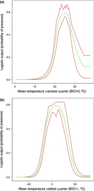
Response curves for the environmental variables that most contribute to the Drosophila americana distribution model when using (a) heat‐related variables and (b) cold‐related variables. The green middle line refers to the average probability of presence estimated from the 10 replicates run with maxent; red lines indicate the maximum and minimum values of the 10 replicates.
Environmental niche models, marginality and specialization of chromosomal forms
The models using the first set of environmental variables had high AUC values (0.943 and 0.987 for americana and texana chromosomal forms, respectively; Table 2a,b). The predicted distribution of the X/4 fused form was larger than that of the nonfused form (Fig. 3). Furthermore, maxent analyses also indicate that the niches of the two chromosomal forms differ in the relevance of precipitation. The mean temperature of the warmest quarter (BIO10) showed contribution values of 47.2% and 39.5% in the americana and texana chromosomal forms' models, respectively (Table 2a,b). The permutation importance of this variable was high with drops of 63.9% and 47.7%, respectively (Table 2a,b). The other variables of relevance in the distribution models of the two forms were different. Thus, the variable that contributes most to the texana model (53.6%) was BIO14 (precipitation of driest month), with a permutation importance of 34%, whereas in americana, the annual precipitation (BIO12) had a contribution of 17.9% but with a low permutation importance (1.3%) (Table 2a,b). In general, most precipitation‐related variables are correlated, making it difficult to unravel the relative importance of each. BIO12 and BIO14 have a Pearson correlation value of 0.71 (Appendix S2). However, the fact that their permutation test vales were different for the models of each chromosomal form suggests that precipitation is more important to the texana than the americana model.
Contribution and permutation importance of the different climatic variables towards the distribution model of (a) americana and (b) texana forms, and results with the alternative cold‐related climatic variables for (c) americana and (d) texana forms. In bold, the variables with the highest contribution for each chromosomal form.
| Variables | Per cent contribution | Permutation importance | Per cent contribution | Permutation importance |
| (a) americana | (b) texana | |||
| Mean temperature warmest quarter (BIO10) | 47.2 | 63.9 | 39.5 | 47.7 |
| Temperature annual range (BIO7) | 20.6 | 17.4 | 1.2 | 2.9 |
| Annual precipitation (BIO12) | 17.9 | 1.3 | 0.6 | 2.3 |
| Precipitation driest month (BIO14) | 6.5 | 6 | 47.2 | 34 |
| Mean diurnal range (BIO2) | 3.6 | 7.2 | 2.1 | 1.8 |
| Precipitation seasonality (BIO15) | 2.8 | 2.2 | 1.4 | 10.7 |
| Mean temperature wettest quarter (BIO8) | 1.6 | 2 | 1.6 | 2 |
| (c) americana | (d) texana | |||
| Mean temperature coldest quarter (BIO11) | 69.6 | 79.3 | 36.5 | 76.3 |
| Mean diurnal range (BIO2) | 21.7 | 15.2 | 4.4 | 2.2 |
| Precipitation seasonality (BIO15) | 4.5 | 2.4 | 12 | 14.3 |
| Precipitation coldest quarter (BIO19) | 4.2 | 3.1 | 47.1 | 7.2 |
| (c) americana | (d) texana | |||
| Mean temperature coldest quarter (BIO11) | 69.6 | 79.3 | 36.5 | 76.3 |
| Mean diurnal range (BIO2) | 21.7 | 15.2 | 4.4 | 2.2 |
| Precipitation seasonality (BIO15) | 4.5 | 2.4 | 12 | 14.3 |
| Precipitation coldest quarter (BIO19) | 4.2 | 3.1 | 47.1 | 7.2 |
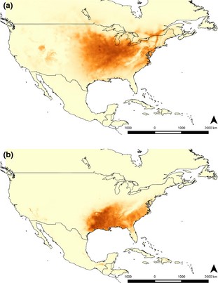
Prediction of present distribution range of (a) americana (X/4 fused form) and (b) texana (unfused form) estimated with maxent using the WorldClim dataset.
Results also showed differences between the two chromosomal forms' models when run with the alternative variables related to minimum temperatures (Table 2c,d). The variable that contributed most to the americana model was the mean temperature of the coldest quarter (BIO11), with a value of 69.6% and a permutation importance of 79.3%, followed by the mean diurnal range (BIO2) with a contribution of 21.7% and a permutation importance of 15.2%. The contribution of BIO11 was expected given its high correlation with BIO10; however, BIO2 showed no correlation > 0.75 to any other bioclimatic variable (Appendix S2). The variable that contributed most to the southern texana form model was the precipitation of the coldest quarter (BIO19), 47.1%, but the permutation importance was only of 7.2%. The second variable in contribution was the mean temperature of the coldest quarter BIO11, with a contribution of 36.5% and a permutation importance of 76.3%. BIO19 probably partly reflects the relevance of BIO14 in the model above as these two variables show a correlation of 0.67.
To further evaluate the differences in environmental conditions endured by the chromosomal forms, we extracted from the variables' response curves the range of values for which the model predicted suitability. In the case of americana, the predicted suitability for BIO10 ranges from 15 to 35 °C, with the maximum probability at 22.5 °C. In the case of texana, the model predicted suitability in BIO10 from approximately 19–35 °C, with the maximum probability at 26.6 °C. In the case of the precipitation during the driest month, the probability of occurrence started to increase at 20 mm, with the probability reaching a plateau at 80 mm. In the analyses using cold‐related variables, americana probability of presence ranged from −15 to 10 °C, with the predictability maximized at about −2 °C. In texana, it ranged from −5 to 22 °C, the probability of presence being maximized at 8 °C. The precipitation of the coldest quarter (BIO19) ranged from 5 mm to > 100 mm.
The differences in environmental niche between the chromosomal forms were further explored using the factor analysis of ecological niche (ENFA). The overall marginality values of the americana and texana forms were positive and relatively high (0.732 and 1.388, respectively), indicating that both occupy suitable areas that deviate substantially from the mean values of the environment available (marginal habitats). The value of marginality was higher in the case of texana, indicating that the level of differentiation between the form's habitat and the study area was higher than in the case of americana. With respect to overall specialization factors, both chromosomal forms showed similar high levels of specialization (4.243 and 4.437 for americana and texana, respectively), suggesting that they are present in a small range of the conditions available in the study area. These results suggest that both taxa have narrow niche breadths.
Models of species past distribution
The suitable habitat available for the species was substantially reduced during the last glacial maximum (LGM, ~21 000 years before present) in comparison with the last interglacial period (LIG ~120 000 to ~140 000 ybp) (Fig. 1c,d). The MIROC model showed a narrow strip of available habitat for the species in the southernmost regions of the USA during the LGM, whereas the CCSM model predicted a complete extinction of the available habitat for the species (map not shown). The area occupied by the species during the LIG was estimated from the distribution maps (no. of pixels × 111.12 km pixel−1) to have been 8441765.99 km2. This area was reduced to 3463.24 km2 during the LGM (MIROC) after which it has increased to the present estimated area of 4125639.86 km2.
Demography of D. americana
Tajima's D and Fu's F values were all negative suggesting a population expansion (Table 3). Deviation from the neutral model was significant for eight genes in the case of Tajima's D (sprk79D, pHCl, CG8398, CG9674, dpr10, nkd, pk61C and tra) and four for Fu's F (pHCl, CG9674, dpr10 and mub). The interpretation of a population expansion is supported by the nonsignificant values of the raggedness index (r) observed in all genes except mub (Table 3).
Tajima's D (D), Fu's F (F) and raggedness (r) test results for each gene. Significant values are shown in bold.
| Gene | D | F | r |
| CG3223 | −0.218 | −0.737 | 0.048 |
| CG9631 | −1.238 | −1.257 | 0.069 |
| Eb | 0.049 | −1.457 | 0.049 |
| tll | −0.521 | −1.778 | 0.045 |
| srpk79D | −1.562 | −6.364 | 0.047 |
| pHCl | −1.615 | −4.982 | 0.056 |
| CG14820 | −0.304 | −3.741 | 0.028 |
| CG7255 | −0.785 | −3.331 | 0.066 |
| CG8398 | −0.854 | −3.361 | 0.076 |
| CG9674 | −1.569 | −5.607 | 0.041 |
| Dpr10 | −1.322 | −6.277 | 0.045 |
| Geko | −0.632 | −4.452 | 0.026 |
| Mub | −0.608 | −5.553 | 0.011 |
| Nkd | −0.476 | −1.390 | 0.026 |
| Pk61C | −1.047 | −7.152 | 0.038 |
| Tra | −0.736 | −21.717 | 0.014 |
Two runs of 500 million generations each were combined to obtain good ESS values (> 200) as estimated with tracer. Multilocus EBSP results show highest posterior probability for two changes in population size. The plot indicates that the population of D. americana has been steadily increasing since its origin, with two expansions occurring around the time of origin ~1 million years before present (mybp) to ~0.7 mybp and at ~300 000 ybp (Fig. 4).
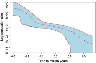
Extended Bayesian Skyline Plot of the Drosophila americana effective population size logarithmically scaled (Y axis) over time indicated in million years before present (X axis). The dashed line is the median population size, and the shaded area corresponds to the 95% HPD (credible intervals).
Thermal performance of the chromosomal forms
Locomotor activity of the flies increased with temperature as shown in the performance plot (Fig. 5; raw values in Appendix S4). The activity remained low between 15 and 25 °C and started to increase at 28 °C reaching a maximum at 38 °C. In the present range of temperatures, the expected rapid decrease in activity after the maximum was not reached, suggesting that the thermotolerance of this species is higher. The two chromosomal forms showed no difference in locomotor activity at the various test temperatures [nonparametric Mann–Whitney U tests with correction for multiple testing (Bonferroni, Holm, Hochberg, Hommel, BH, BY and SGoF); Table 4].
Average activity counts, estimated as the average number of times a fly crosses the beam in the DAM, and standard deviation, for each chromosomal form at different temperatures tested. P shows the probability values of Mann–Whitney U test after Bonferroni correction (less conservative methods for multiple test correction also result in adjusted P > 0.05, see text).
| Temp. (°C) | americana | texana | P |
| Activity counts (SD) | Activity counts (SD) | ||
| 15 | 6.6667 (24.4274) | 3.1964 (12.7214) | 1 |
| 18 | 6.3153 (17.4913) | 4.3929 (17.3877) | 1 |
| 20 | 10.3694 (25.1638) | 4.8571 (16.6911) | 0.05598 |
| 22 | 4.9459 (16.2815) | 3.1786 (9.4471) | 1 |
| 25 | 5.8288 (14.6516) | 7.4732 (17.4789) | 1 |
| 28 | 12.3784 (35.0042) | 24.2500 (58.4156) | 0.85833 |
| 30 | 30.4144 (36.5077) | 40.5000 (50.7497) | 1 |
| 35 | 89.9369 (55.7839) | 77.0893 (48.1601) | 0.51741 |
| 38 | 120.5315 (57.5645) | 102.1518 (54.8811) | 0.12942 |
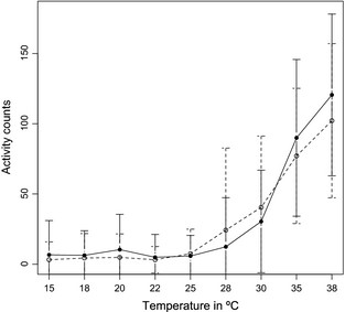
Average activity count and standard deviation (vertical bars) plot at the different temperatures tested. americana – solid line, texana – dashed line.
Developmental time and fertility/viability of the chromosomal forms
There were significant differences in males' DT within chromosomal forms at different temperatures and between chromosomal forms at the same temperature (Mann–Whitney U test P < 0.001; Table 5; number of individuals and number of vials needed to obtain it are shown in Appendix S5). DT was higher at 22.5 °C and decreased on average 3.1 and 4.0 days at 26.6 °C for americana and texana chromosomal forms, respectively (Table 5). Males from the americana chromosomal form developed faster on average than texana males. The differences in DT between chromosomal forms reached 1.2 days at 22.5 °C and 0.4 at 26.6 °C.
Average developmental times (DT) and standard deviation (SD) estimated as the number of days between egg laying and adult emergence, for each chromosomal form (americana and texana) at the two temperatures (Temp.) tested. N, number of male flies emerged. P shows the probability values of Mann–Whitney U test after Bonferroni correction.
| Temp. (°C) | americana | texana | P | ||
| DT (SD) | N | DT (SD) | N | ||
| 22.5 | 17.0 (1.1) | 651 | 18.3 (1.9) | 872 | < 0.001 |
| 26.6 | 13.9 (1.6) | 771 | 14.3 (1.5) | 427 | < 0.001 |
| Temp. (°C) | americana | texana | P | ||
| DT (SD) | N | DT (SD) | N | ||
| 22.5 | 17.0 (1.1) | 651 | 18.3 (1.9) | 872 | < 0.001 |
| 26.6 | 13.9 (1.6) | 771 | 14.3 (1.5) | 427 | < 0.001 |
Statistically significant differences in fertility/viability were found within chromosomal forms at both experimental temperatures (22.5 °C vs. 26.6 °C; = 7.64, P < 0.01 and = 99.82, P < 0.001 for americana and texana, respectively; Table 6a). On average, a decrease in one degree corresponded to an increase of 4.2% and 19.5% in viability for the americana and texana chromosomal forms, respectively. A statistically significant difference in fertility/viability was also found when comparing americana and texana at 22.5 °C ( = 100.36, P < 0.001; Table 6b), but not at 26.6 °C ( = 1.69, P = 0.193; Table 6b).
Comparison of the fertility/viability estimates within chromosomal forms at different temperatures (a) and between chromosomal forms at the same temperature (b).
| (a) | ||||||||||
| Chrom. | 22.5 °C | 26.6 °C | Chi | P | ||||||
| N | E | T | R | N | E | T | R | |||
| americana | 651 | 599.5 | 121 | 5.4 | 771 | 822.5 | 166 | 4.6 | 7.64 | < 0.01 |
| texana | 872 | 692.3 | 97 | 9.0 | 427 | 606.7 | 85 | 5.0 | 99.82 | < 0.001 |
| (a) | ||||||||||
| Chrom. | 22.5 °C | 26.6 °C | Chi | P | ||||||
| N | E | T | R | N | E | T | R | |||
| americana | 651 | 599.5 | 121 | 5.4 | 771 | 822.5 | 166 | 4.6 | 7.64 | < 0.01 |
| texana | 872 | 692.3 | 97 | 9.0 | 427 | 606.7 | 85 | 5.0 | 99.82 | < 0.001 |
| (b) | ||||||||||
| Temp. (°C) | americana | texana | Chi | P | ||||||
| N | E | T | R | N | E | T | R | |||
| 22.5 | 651 | 845.3 | 121 | 5.4 | 872 | 677.7 | 97 | 9.0 | 100.36 | < 0.001 |
| 26.6 | 771 | 792.3 | 166 | 4.6 | 427 | 405.7 | 85 | 5.0 | 1.69 | > 0.193 |
| (b) | ||||||||||
| Temp. (°C) | americana | texana | Chi | P | ||||||
| N | E | T | R | N | E | T | R | |||
| 22.5 | 651 | 845.3 | 121 | 5.4 | 872 | 677.7 | 97 | 9.0 | 100.36 | < 0.001 |
| 26.6 | 771 | 792.3 | 166 | 4.6 | 427 | 405.7 | 85 | 5.0 | 1.69 | > 0.193 |
Chrom., chromosomal form; Temp., temperature; Chi, value of χ2; P, Probability; N, number of males; E, expected number of males under the assumption of no differences in fertility/viability between the cells being compared; T, number of vials needed to get N flies; R is N/T. All significant values remain significant after Bonferroni correction for multiple testing.
Discussion
Temperature is commonly considered to be the main variable shaping the geographical distribution of Drosophila species. Although previous work has focused on populations from different latitudes assuming that temperature was the main factor affecting the individual fitness, there are no studies addressing the relevant environmental variables that drive the ecological niche of Drosophila in natural populations. In this study, we showed that temperature is the main limiting climatic variable of those included in the ecological niche model (ENM) of D. americana. This is also true when considering the two chromosomal forms (X/4 fusion, americana form and X free, texana form) separately, although precipitation also plays a major role in the ecological niche model of the southern, texana form. These results are in agreement with the previous study by McAllister et al. (2008), who found a correlation between the frequency of the X/4 chromosomal rearrangement and the minimum temperature of January. The ENMs revealed a difference of 4 °C between the texana and americana optimal model temperatures in the case of the warmest quarter (22.5 and 26.6 °C for americana and texana, respectively) and of 10 °C in the coldest quarter (−2 and 8 °C for americana and texana, respectively). The model temperature response curves largely overlap for the two forms, which is in agreement with the north–south clinal distribution of the X/4 chromosomal rearrangement. Overall, results indicate that the northern and southern populations of D. americana are subject to slightly different but overlapping environmental ranges. Nevertheless, the climatic factors that drive their ecological niches differ in their relevance. The southern form is more dependent on precipitation than the northern form, whose model is preferentially driven by temperature, suggesting a difference in their niche preference.
Populations can respond differently to the varying climatic conditions occurring in their ranges. For instance, there is evidence for the adaptation of Drosophila populations to different temperatures along latitudinal gradients and between tropical and temperate populations (Balanyà et al., 2003; Trotta et al., 2006; McAllister et al., 2008; Rezende et al., 2010; van Heerwaarden & Sgro, 2013). In addition, there is evidence that behavioural plastic responses are of relevance when coping with temperature differences (Austin & Moehring, 2013; Castañeda et al., 2013). In the case of D. americana, it has been previously suggested that the alternative chromosomal rearrangements influence divergent overwintering strategies and may represent the early stages of ecological speciation (McAllister et al., 2008). However, the question of whether populations of this species are differentially adapting to their respective niches has, so far, not been investigated. Although ENMs showed different variables of varying importance, we observed no significant differentiation between forms in locomotor activity at the various temperatures tested. This suggests that optimal body temperature for locomotor performance does not differ between adult males of the two chromosomal forms, although longer exposure to the different temperatures could uncover as yet undetected differences. However, there is no evident tendency towards different preferred temperatures for each form after 35 min of exposure while there is a clear increase in activity with temperature. If 35 min were not sufficient to elicit a locomotor response, we would not expect to observe a tendency in the temperature preference gradient either. Results, thus, suggest that there is no evident differential adaptation in the locomotor activity optimal body temperature between the chromosomal forms, which could suggest a role for behavioural thermoregulation in adult flies for this trait.
In contrast, we found significant differences in the developmental time and fertility/viability between and within chromosomal forms at the optimum mean temperatures of the warmest quarter as inferred from their respective models. These results indicate that performance of D. americana related to these traits is clearly dependent on temperature, as in the case of other species, such as D. melanogaster and D. simulans (James et al., 1997; Petavy et al., 2001; Trotta et al., 2006). However, our results show that the populations are not optimally adapted in these traits to the average environmental temperatures they encounter in their distribution area. Thus, developmental time is significantly lower in both chromosomal forms at 26.6 °C than at 22.5 °C, and viability/fertility is significantly smaller at 26.6 °C than at 22.5 °C. If chromosomal forms were differentially adapted in these traits, the direction of change from one temperature to the other should be opposite in each chromosomal form. This is not observed, showing no evidence for differential adaptation to the local environment in the traits studied here. However, these results do not eliminate the possibility of thermal adaptation in other traits that we have not measured. In Drosophila, there is a trade‐off between fecundity and survival that is mediated through body size and developmental time (Roff, 1981). Thus, given that the americana form develops faster and still has a similar fecundity at 26.6 °C when compared to the southern texana form, the americana form would be expected at higher frequencies in the southern populations than it is observed. This points towards a disadvantage with respect to the local texana form in some other traits not studied in the present work.
In the case of D. americana, the width of the locomotor activity curve is small, and developmental time (DT) as well as fertility/viability is significantly reduced within a narrow range of temperatures. This indicates a narrow thermal range in comparison with that observed in other species such as D. melanogaster and D. simulans (Petavy et al., 2001). The thermal range of D. americana is also in agreement with the observed values of marginality and specialization obtained with the ENFA analyses, which suggest a narrow niche breadth and marginal habitat in contrast to the distribution model's predicted range of temperatures. This observation could be explained if phenotypic plasticity and/or behavioural thermoregulation at the microhabitat level were relevant in the thermal adaptation process of D. americana, and therefore in its latitudinal geographical distribution.
According to the realized niche models, the suitable distribution for D. americana during the last interglacial period [LIG; ~140 000 to ~120 000 years before present (ybp)] is predicted to have been twice the size of the current one. The models also predicted a drastic reduction in the suitable area for D. americana during the last glacial maximum (LGM) ~21 000 ybp, which suggest a strong bottleneck during that period followed by a recent (< 21 000 ybp) expansion to the present day distribution, approximately 1190 times larger. However, there is no evidence from the DNA analyses for a bottleneck during the LGM, but rather demographic expansions of the population of D. americana around 1–0.7 mya and 300 000 ybp. The lack of support for a LGM bottleneck with post‐glacial expansion is in agreement with previous studies that concluded that the species had a stable recent historical population size (Schäfer et al., 2006; Morales‐Hojas et al., 2008). Other studies suggest a fairly large recent increase in population size within a time span of approximately 0.11 × 2Ne generations, corresponding to approximately 61 600 ybp (de Proce et al., 2012). This estimate relies, however, on the assumption of an effective population size that is 38% of that recently estimated for this species based on a much larger polymorphism dataset and the sequence of two genomes (Fonseca et al., 2013). Therefore, the expansion may have occurred as long as 79 200 ybp, under the assumption of five generations a year (as in de Proce et al., 2012), but it could be as old as 99000 ybp under the assumption of eight generations a year, based on developmental time data for D. americana obtained in this study and that estimated by Fonseca et al. (2013). In any case, the demographic history of this species as estimated from molecular data is not detecting a bottleneck during the last glaciation (~21 000 ya). Contradictory results between species' past distribution inferred from the ENMs and the demographic history inferred from the DNA‐based analyses could be an indication of the absence of niche conservatism in this species. Under this scenario, the populations of D. americana would have been able to respond to different climatic conditions from those that comprise their present niches. This explanation would support the idea that niche preference of D. americana evolves as a response to environmental change through time, and behavioural thermoregulation probably plays a key role in this capacity to respond to the diverse climatic conditions it encounters. However, there are other possibilities that would explain the contradictory results between the niche models and the molecular data. If the genetic diversity of the species had recovered rapidly after the bottleneck, its molecular signature would be lost. Two possible scenarios would meet this condition: (i) there were more than one refuge for the species during the LGM, and after the ice retreated the genetically differentiated populations mixed rapidly, increasing the genetic diversity of the species; (ii) there was one single population, and its effective population size was sufficiently high to prevent a drastic reduction in the genetic diversity of the species. Results from the ENM using the MIROC model show at least three main isolated areas suitable for the species (Fig. 1c), which would support the first scenario over the latter. A third possible explanation, compatible with the previous two, relates to the assumption that the past and current land surfaces of North America are equal. As the glaciers increased in volume, the sea level dropped exposing new land surface. Thus, the real reduction in habitable area for the species may have not been as drastic as predicted by the past projection of the model, and the species would have occupied areas now under water, maintaining a large effective population size throughout the LGM.
In conclusion, there is no evidence for local divergent adaptation in the traits studied here to the different environmental conditions observed along the species' geographical range. However, we cannot reject the possibility of local adaptation along the latitudinal gradient occurring in other traits not included in the present study. The inconsistent results between the demographic molecular analyses and the predicted past species' distribution models suggest that this species has a capacity to respond to different environmental conditions, supporting a role for behavioural thermal regulation. Nevertheless, there are some caveats in the molecular analyses and further sampling will be fundamental to fully comprehend the phylogeographical history of the species.
Acknowledgments
This work was funded by FEDER Funds through the Operational Competitiveness Programme – COMPETE and by national funds through FCT – Fundação para a Ciência e a Tecnologia under the projects FCOMP‐01‐0124‐FEDER‐037277 (PEst‐C/SAU/LA0002/2013) and a PhD grant attributed by FCT with the reference SFRH/BD/61142/2009 to M.R. We would like to thank Robert A. Cheke for his revision and comments to the manuscript.
References
Author notes
These two authors have equally contributed to the work
Co‐senior authors
Data deposited at Dryad: doi: 10.5061/dryad.5ng71
