


ABSTRACT
In preclinical models, the composition and function of the gut microbiota have been linked to bone growth and homeostasis, but there are few available data from studies of human populations. In a hypothesis‐generating experiment in a large cohort of community‐dwelling older men (n = 831; age range, 78–98 years), we explored the associations between fecal microbial profiles and bone density, microarchitecture, and strength measured with total hip dual‐energy X‐ray absorptiometry (DXA) and high‐resolution peripheral quantitative computed tomography (HRpQCT) (distal radius, distal and diaphyseal tibia). Fecal samples were collected and the 16S rRNA gene V4 hypervariable region sequenced. Sequences were bioinformatically processed through the DADA2 pipeline and then taxonomically assigned using SILVA. Generalized linear models as implemented in microbiome multivariable association with linear models (MaAsLin 2) were used to test for associations between skeletal measures and specific microbial genera. The abundances of four bacterial genera were weakly associated with bone density, structure, or strength (false discovery rate [FDR] ≤ 0.05), and the measured directions of associations of genera were generally consistent across multiple bone measures, supporting a role for microbiota on skeletal homeostasis. However, the associated effect sizes were small (log2 fold change < ±0.35), limiting power to confidently identify these associations even with high resolution skeletal imaging phenotypes, and we assessed the resulting implications for the design of future cohort‐based studies. As in analogous examples from genomewide association studies, we find that larger cohort sizes will likely be needed to confidently identify associations between the fecal microbiota and skeletal health relying on 16S sequencing. Our findings bolster the view that the gut microbiome is associated with clinically important measures of bone health, while also indicating the challenges in the design of cohort‐based microbiome studies. © 2022 American Society for Bone and Mineral Research (ASBMR).
Introduction
Complex multicellular organisms exist as a symbiosis between the host and resident microbiota. The largest portion of the human microbiota is in the gut, which is also responsible for the majority of immune, metabolic, and biochemical host‐microbial interactions.(1) As a result, the composition of the gut microbiota has been linked to a wide variety of normal physiological processes outside the intestine, disturbances have been implicated in the causation of numerous disorders, and there may be many opportunities to therapeutically alter microbiota composition or function.(2) Due to the diversity of microbial chemistry and the lifelong nature of association with a personalized gut microbiome, gut microbes could participate in health phenotypes that might be unexpected, such as kidney stone formation, inorganic detoxification, and developmental processes.(3,4)
Skeletal homeostasis appears to be affected by the gut microbiota.(5‐7) A number of critical experiments in laboratory animals have revealed skeletal effects of changes in gut microbiota composition. Germ‐free mice can have altered bone characteristics, including increased bone density.(8‐11) However, these findings are not consistently present,(12‐14) and as with many gnotobiotic animal settings, different outcomes are potentially related to the background strains of the animals used, the protocols for the studies, the age or sex of animals, housing conditions, etc. Similarly, antibiotic treatments have been shown to have a range of effects on bone density; antibiotic‐treated mice appear to have higher bone density in some experiments,(12) but other reports include adverse(15,16) or no effects.(17) Finally, a number of experiments have demonstrated that probiotic preparations, commonly including one or more Lactobacillus species, may positively affect mineral metabolism or bone health.(18‐21)
Despite the growing series of animal experiments that demonstrate an effect of the gut microbiome on skeletal health, there are very few studies in humans that examine whether there are associations between the gut microbiome and skeletal status. Wang and colleagues(22) reported the relationship between categories of BMD (primary osteoporosis, osteopenia, normal based on dual‐energy X‐ray absorptiometry [DXA]) in a very small number of participants (three male and 15 female patients), but there are no studies in larger cohorts. Jones and colleagues(13) recently summarized compelling studies that suggest that the critical adverse skeletal effects of oophorectomy, and the positive effects of some probiotics, are at least in part mediated via alterations the gut microbiota, gut permeability, and immune function. The mechanisms that mediate the interaction between the gut microbiota and bone are undoubtedly complex, but may involve combinations of immune function and inflammation,(12,23‐25) changes in endocrine factors,(26,27) nutritional effects and prebiotics,(28‐34) secreted microbial products,(35,36) effects mediated by exercise,(37) and others.(5,14,20,27,38,39)
We thus aimed to test for covariation between the gut microbiome and skeletal biology in humans by studying the associations of the fecal microbiome with multiple measures of bone density, microarchitecture, and strength in a large cohort of community dwelling older men. We obtained stool samples from 831 participants in the Osteoporotic Fractures in Men (MrOS) study—a longitudinal observational study of musculoskeletal health and aging.(40,41) We then performed 16S rRNA amplicon sequencing, and tested for associations between the abundance of microbial clades and human bone measures obtained with high‐resolution peripheral quantitative computed tomography (HRpQCT) and DXA. We viewed this experiment as exploratory and hypothesis generating. Because the resulting associations were of generally small effect, we utilized this experience to explore the implications for the design of future cohort‐based microbiome studies specifically planned to confidently identify microbiome compositions that are associated with skeletal traits.
Subjects and Methods
Participants: the MrOS cohort
The MrOS study is a prospective study of 5994 community‐dwelling older men, recruited at six clinical sites in the United States between 2000 and 2002. The cohort and recruitment methods have been described.(40,41) At baseline, participants were at least 65 years of age, able to consent, walked without assistance of another person, and did not have bilateral hip replacement or any condition that in the judgment of the site investigator that would likely impair participation in the study. The Institutional Review Boards at all sites reviewed and approved the study and all participants provided informed consent. All surviving active MrOS participants were invited to participate in a year 14 visit occurring between May 2014 and May 2016.
As part of a microbiome study, 1329 of the men participating in the visit were invited to provide a stool sample starting in 2015. Some men (347) refused or were deemed ineligible to collect specimens because of cognitive or physical limitations that interfered with the sample collection, 982 participants agreed, 951 specimens were obtained, 31 specimens were inadequate, and one did not pass the pipeline validation code after genotyping; thus, 919 had complete microbiome data available (Fig. 1). There were a few small but significant differences between those who agreed and those who refused: the men who agreed were slightly younger, more active, stronger, and more often reported good or excellent health than those who declined.(42) Participants were also queried about antibiotic use in the 30 days prior to sample collection, and the 66 (7.2%) who reported use were excluded from the analyses. Finally, complete covariate data were missing in 22. Thus, the final analyses included 831 participants.
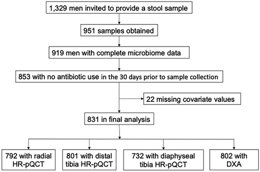
Selection of participants; fully described in Subjects and Methods.
Microbiome sample collection, 16S rRNA gene sequencing, and sequence data processing
As described,(42) after collection instructions were provided during the in‐person clinic visit, fecal samples were collected by study participants at their homes using the Omnigene Gut collection kit (OMR‐200; DNA Genotek, Ottawa, Canada) that includes a stabilizing reagent to preserve stool DNA at ambient temperature for up to 60 days.(43,44) Stool collection was within 1 month after the study visit for 98.3% of participants, and others were within 3 months. Samples were mailed directly to Portland and stored at −80°C until DNA extraction. The specimens were sent to the Alkek Center for Metagenomics and Microbiome Research (CMMR), Baylor College of Medicine in Houston, TX, USA, where the samples were aliquotted and genomic bacterial DNA was extracted using the MO BIO PowerSoil DNA Isolation Kit (MO BIO Laboratories, Inc, Carlsbad, CA, USA). The 16S rRNA gene V4 hypervariable region (hereafter abbreviated 16S) was then amplified using primers 515F and 806R by polymerase chain reaction and sequenced on the MiSeq platform using the 2 × 250‐bp paired‐end protocol (Illumina, San Diego, CA, USA). The fecal samples were extracted, amplified, and sequenced in two batches: the first 599 men from whom fecal samples were collected, and those 320 from whom samples were received thereafter. Collection, sample processing, and 16S amplification and sequencing procedures were identical in the two subcohorts. The clinical characteristics of the men in the two batches were highly similar, and microbiome diversity was minimally different between the two batches of samples. Specifically, Shannon alpha diversity (for methods, see Statistical Analyses below) was minimally, albeit significantly, different (batch 1: median Shannon diversity index 3.66; batch 2: 3.76, p = 0.006). Thus, all analyses were performed using the results from the two batches combined, with adjustment for batch in all analyses. In the analyses, no significant batch effects were seen with HRpQCT measures.
Raw amplicon sequences as FASTQs were then bioinformatically processed through the DADA2(45) workflow in R which has been wrapped in the reproducible bioBakery workflow(46) with AnADAMA2. Briefly, sequences are demultiplexed, after which DADA2 de‐noising, filtering, trimming, merge, chimera removal, and taxonomic classification is executed in R (R Foundation for Statistical Computing, Vienna, Austria; https://www.r-project.org/) using default parameters for paired‐end Illumina sequence data. DADA2 assesses the reads for sequence error rates and corrects on a base‐by‐base basis. Chimera removal occurs while simultaneously assigning amplicons to amplicon sequence variants (ASVs). Assigning ASV is based on determining which exact sequences were read and how many times each was read. These data are then combined with an error model for the sequencing run, enabling the comparison of similar reads to determine the probability that a given read at a given frequency is not due to sequencer error. Phylogenetic trees are constructed after alignment of sequences using Clustal Omega.(47) ASVs are then taxonomically assigned using the SILVA(48) reference database (version 128).
This yielded a total of 12855 denoised ASVs across all samples, with an average of 25487 reads per sample (ranging from 5429 to 70721 reads). ASVs were excluded if present in <10% of samples or at a relative abundance of <0.0001, leaving 2788 available for analysis after quality control.
Skeletal measures
HRpQCT measures were performed using Scanco XtremeCT II machines (Scanco Medical AG, Brüttisellen, Switzerland) as described.(49) Centrally trained operators acquired scans of the distal radius (9 mm from the articular surface), distal tibia (22 mm from the articular surface), and diaphyseal tibia (centered at 30% of tibial length, as measured externally from the tibial plateau to the tibial malleolus. The radius from the nondominant arm and the tibia from the ipsilateral leg were scanned except in the case of prior fracture, metal shrapnel or implant, or recent non‐weight‐bearing status persisting >6 weeks; 8% of radius scans and 8% of tibia scans were performed on the dominant limb. Machines were calibrated prior to being used in the present study, and a single cross‐calibration density phantom was circulated among the study sites.
Centralized quality assurance and standard analysis of all image data, including micro‐finite element analysis (μFEA), was performed. A central observer read all images for motion artifacts and used an established semiquantitative five‐point grading system (1 = superior, 5 = poor) to score image quality; images of grade 4 or 5 were deemed to be of insufficient quality and were excluded from the analytic data set (97% of scans had image grade ≤ 3). The final analyses included 792 radial, 801 distal tibial, and 732 proximal tibial images (Fig. 1).
A fully automated analysis pipeline was developed to segment the radius and tibia for quantification of bone density and microarchitecture. Volumetric bone mineral density (BMD) and cross‐sectional area of the total, cortical, and trabecular compartments were measured. Cortical porosity and thickness, and trabecular thickness and number were calculated directly. Linear elastic μFEA of a 1% uniaxial compression was performed using a homogenous elastic modulus of 10 GPa and a Poisson's ratio of 0.3 (Scanco FE Software v1.12; Scanco Medical). The failure load was estimated by calculation of the reaction force at which 7.5% of the elements exceed a local effective strain of 0.7%. The measures were identified as suggested by Whittier and colleagues.(50) The precision of HRpQCT measures have been reported.(51,52) Because associations of bone measures with the gut microbiome may be different depending on the specific site of measurement (eg, cortical versus trabecular, radial versus tibial) we examined these associations using several types of bone measures. In that analytical context, the intercorrelations between measurement sites should also be considered; those intercorrelations are shown in Supplemental Fig. 1.
Hip DXA scans were performed on Hologic 4500 scanners (Hologic, Waltham, MA, USA) as described.(53) Centralized quality‐control procedures, certification of DXA operators, and standardized procedures for scanning were used to ensure reproducibility of DXA measurements. The coefficient variation of the MrOS DXA scanners estimated using a central phantom ranged from 0.3% to 0.7% for the total hip. Each participant's right hip was scanned unless there was a fracture, implant, hardware, or other problem preventing the right hip from being scanned; in those instances, the left hip was scanned.
Other measurements
Body weight was measured on balance beam or digital scales; height was measured using a Harpenden stadiometer (Holtain, Dyfed, UK). Body mass index (BMI) was calculated as weight (kg)/height (m2). Medical history included self‐reported physician diagnosis of diabetes. Alcohol use was assessed as 0–5 or ≥6 drinks/week. All men completed questionnaires and were interviewed about health status, including an assessment of life space.(54) Each self‐reported his health as excellent/good, fair, poor, or very poor. The Physical Activity Scale for the Elderly (PASE) questionnaire was used to estimate physical activities.(55) All prescription medications were recorded in an electronic medication inventory database and matched to its ingredients based on the Iowa Drug Information Service drug vocabulary (College Pharmacy, University of Iowa, Iowa City, IA, USA).(56) The composite life space score, a comprehensive measure of mobility that captures an individual's movement in their environment, was assessed by questionnaire.(54) Diet was assessed using the Block dietary questionnaire, and the response data was reduced using factor analyses to derive two major dietary patterns (“Western” and “prudent”),(57,58) which were used as covariates in these analyses. They represent two dietary patterns that are commonly empirically derived based on the underlying distribution of the dietary habits of participants. The Western dietary pattern is characterized by high intakes of processed meat, fried foods, snacks, and desserts. The prudent dietary pattern is characterized by high intakes of fruits, vegetables, legumes, whole grains, and lean meats like chicken. The scores are a linear combination of foods in that pattern; a higher factor score indicates a higher correlation of foods in that dietary pattern.
Statistical analyses
The analytic sample for the present analysis included those 831 men with 16S sequencing and measures of bone parameters who reported no use of antibiotics within the past month and complete data for the adjustment covariates (Fig. 1). The Kruskal‐Wallis test was used to determine differences in categorical demographic and clinical covariates such as age, race, diet, BMI, and clinic site.
Diversity analyses
Alpha diversity (estimated using the Shannon index) is a measure of the richness of a microbial community (total number of taxa and evenness of the taxa present) in a single sample. We tested for alpha diversity associations with HRpQCT measures using linear regression controlling for covariates (age, race, clinic site, diet, and BMI).(57,59) Beta diversity estimates (measures of the differences in microbial abundance between two samples) included Bray‐Curtis dissimilarity and unweighted and weighted UniFrac distance metrics. Weighted‐UniFrac takes into account the relative abundance of species/taxa shared between samples, whereas unweighted‐UniFrac only considers presence/absence. Principal coordinates analysis (PCoA) was used to analyze and visualize patterns of beta diversity in sequence count data. To prepare the analytic data set from raw ASV count data we agglomerated ASVs to the genus level, filtered the resulting taxa (requiring at least 10% prevalence and 0.0001 abundance) and used relative abundance to normalize; ie, control for differences in library sizes. We did not rarefy to equalize counts for any of the analyses. The final dataset included 122 total ASVs. Permutation analysis of variance (PERMANOVA) as implemented by the adonis function in R vegan was used to test the statistical significance of microbial community dissimilarities across continuous bone measures with 999 permutations.
Associations between microbial abundance and skeletal measures
For association analyses, counts were filtered and then agglomerated (final dataset, 129 ASVs). Generalized linear models as implemented in Microbiome Multivariable Association with Linear Models (MaAsLin 2) were used to test for associations between skeletal measures and specific microbial genera.(60) Bacterial count data were normalized and transformed according to methods available in the package (CSS normalization and log transformation). The default MaAsLin 2 parameters were applied (taxonomic feature prevalent in a minimum of 10% of all samples, minimum percentage relative abundance 0.01%, p < 0.05, q < 0.25). Models used each genus as the outcome (all ASVs for the same genus were agglomerated) and the standardized phenotypes as predictors of interest; ie, the association of the relative abundance of the microbe per SD increase in the bone phenotype. False discovery rate (FDR) values for discovery using MaAsLin 2 were calculated with respect to the set of associations for each skeletal measurement site individually (Table 2). All models were additionally adjusted for age, race, clinic site, diet, BMI, batch number, PASE score, self‐rated overall health, self‐rated diabetes, alcohol use, and number of medications used.
We also evaluated our confidence in the associations of genera with skeletal measures using established approaches for examining local FDR considerations that are similar to those applied to genome association studies,(61‐63) essentially by examining the overall distribution of Z‐scores of associations to determine the degree to which effect estimates in the tails of the Z‐score distribution were expected (followed the theoretical normal null distribution) or unexpected (likely to be non‐null). We used these analyses to estimate the attained power of our study design, and finally considered the power needs of similar future studies. In fact, the observed Z‐score distribution has somewhat long and asymmetrically dense tails (Supplemental Fig. 2), suggesting that at least a proportion of these extreme values (either positive or negative) may represent meaningful associations. Detailed methods for these analyses of the distribution of Z‐scores are provided in Supplemental Statistical Methods. Briefly, we performed a finite mixture analysis of the association Z‐scores, assuming a three‐component mixture where the central component (centered near zero) is normally distributed and represents the “null” associations, and the outer (extremal right and left) components represent the admixture of “non‐null” associations hidden within the tails of the observed distribution. Based on the empirical spread of all the Z‐scores (from all bone measures) taken together, we fit a normal distributional curve to the central (“null”) component and extrapolated that curve into the tails to yield the distribution of Z‐scores that would be expected under the null hypothesis (of no association), given the observed data. At each end of the mixture distribution of the observed Z‐scores, we identified regions in the tails that showed higher density than expected from the normal null distribution and were thus more likely to contain high concentrations of non‐null associations. These components of the mixture were considered “enrichments” (of extreme positive or negative values occurring at higher rates than expected for null associations). To clarify the power of our study design and the challenges in interpreting “significant” effects that may or may not represent real associations, we estimated the expected local FDR value for a non‐null effect appearing in an enriched area of one of the tails of the Z‐score distribution. The local FDR differs from the typical FDR adjustments applied to p values in that the local FDR applies to each Z‐score individually, and is conditioned on that value; it is interpretable as an empirical Bayes probability that the specific Z‐score of interest is a false finding, ie, that it comes from the null distribution rather than from a component of enrichment (typical FDR adjustments, eg, the Benjamini‐Hochberg algorithm, only estimate the average false discovery rate expected across all “discoveries” with a p value more extreme than some cutoff; they are not true probabilities and do not apply to individual results). The expected local FDR for a non‐null effect is the average local FDR value for Z‐scores coming strictly from an enrichment, given the estimated locations of the enrichment components. The higher the expected local FDR value, the lower the power to discover true effects using FDR‐based cutoff criteria (because the probability that any given finding comes from the null distribution instead is high on average).
Visualization of clusters of phenotypes and taxa of interest: Differences in microbial composition per standard deviation of each HRpQCT measure were assessed using the multivariable MaAsLin 2 analysis, and the log2 fold change and FDR‐adjusted p value for each taxon were used to create a heatmap. We performed a hierarchical clustering analysis to group associations found using MaAsLin 2 across the variety of skeletal measures (HRpQCT and DXA). We used Cronbach's alpha to assess the coherence of associations within clusters; we probed the volatility of the alpha coefficient to small amounts of shuffling of the components of the clusters.
Analyses were performed using R version 3.6.0 for processing the microbiome data, diversity analysis were performed using the Phyloseq package in R, regression analysis of the ASVs with the bone phenotypes were performed using the MaAsLin 2 package in R, heatmaps were created using the heatmap2 package in R, Stata version 16.1 (StataCorp, LLC, College Station, TX, USA) was used for the finite‐mixture analysis of association Z‐scores and meta‐analysis of effect sizes across measurement sites, and SAS version 9.4 (SAS Institute, Inc., Cary, NC, USA) was used for creating summary tables.
Results
Participants
Samples adequate for amplicon sequencing were available from 919 men. A number of men were excluded for use of antibiotics and some outcome measurements were missing in additional participants (Fig. 1); the final analyses included data from 831. The clinical characteristics of these men are provided in Table 1, where we also provide a summary of the diversity measures and the average number of amplicon sequence variants (ASVs) detected. Within this population, none of the skeletal measures were significantly associated with alpha diversity (Shannon diversity; Supplemental Table 1) or beta diversity (examples in Supplemental Fig. 3).
Cohort Characteristics (n = 831)
| Characteristic | Value |
| Age (years) | 84.2 ± 4 |
| BMI (kg/m2) | 27 ± 3.7 |
| PASE score | 123 ± 66 |
| Self‐rated health status, n (%) | |
| Excellent/good | 744 (90) |
| Fair, poor, or very poor | 87 (10) |
| Diabetes, n (%) | 124 (15) |
| Alcohol, n (%) | |
| 0–7 (drinks/week) | 503 (60) |
| >7 (drinks/week) | 326 (40) |
| Western diet | −0.03 ± −1.0 |
| Prudent diet | −0.01 ± −1.0 |
| Total number of medications taken | 9 ± 6 |
| Composite life‐space score | 85 ± 22 |
| Shannon alpha diversity* | 3.6 ± 0.6 |
| Observed amplicon sequence variants (ASVs)*, n (range) | 144 (48) |
| Min Bray–Curtis dissimilarity* | 0.6 ± 0.05 |
| Distal radial | |
| Failure load (FL) (kN) | 4921 ± 1344 |
| Total BMD (Tt.BMD) (mg HA/cm3) | 276 ± 60 |
| Trabecular BMD (Tb.BMD) (mg HA/cm3) | 170 ± 39 |
| Trabecular number (Tb.N) (1/mm) | 1.4 ± 0.2 |
| Cortical thickness (Ct.Th) (mm) | 1.0 ± 0.2 |
| Cortical porosity (Ct.Po) (%) | 0.02 ± 0.01 |
| Distal tibial | |
| Failure load (FL) (kN) | 4921 ± 1344 |
| Total BMD (Tt.BMD) (mg HA/cm3) | 276 ± 60 |
| Trabecular BMD (Tb.BMD) (mg HA/cm3) | 170 ± 39 |
| Trabecular number (Tb.N) (1/mm) | 1.4 ± 0.2 |
| Cortical thickness (Ct.Th) (mm) | 1.0 ± 0.2 |
| Cortical porosity (Ct.Po) (%) | 0.02 ± 0.01 |
| Total hip BMD (gm/cm2) | 0.94 ± 0.15 |
Values are mean ± SD or n (%).
Skewed data reported as mean and inter‐quartile range.
Associations between genera and skeletal measures
After multivariable adjustment, we identified possible associations between skeletal measures and specific bacterial genera (Table 2). At MaAsLin 2‐derived FDR ≤ 0.05, the abundances of four genera were associated with one or more skeletal measurement sites: greater Anaerofilum abundance was associated with lower radial and tibial density, radial and tibial strength, tibial cortical thickness and cortical porosity, and hip DXA BMD; Methanomassiliicoccus was associated with greater distal tibial cortical porosity. On the other hand, Ruminiclostridium 9 was associated with less distal tibial cortical porosity, and Tyzzerella with greater tibial density measures. The abundances of two additional genera were associated using a slightly less strict criterion (FDR ≤ 0.1): Lactobacillus and Streptoccocus were both associated with worse bone measures at radial and tibial sites. As this was intended to be an exploratory analysis, Table 2 also includes associations with FDR up to 0.25.
Associations Between Taxa Abundance and Bone Measures From the MaAsLin Multivariate Adjusted Model
| Genus | Mean relative abundance* | Bone phenotype | Log 2 fold change** | FDR q value*** |
| Anaerofilum | 0.00028 | FL distal radius | −0.262 | 0.019 |
| BMD DXA THD | −0.249 | 0.027 | ||
| FL distal tibia | −0.214 | 0.075 | ||
| Ct.Th distal radius | −0.189 | 0.136 | ||
| Tt.BMD distal radius | −0.184 | 0.148 | ||
| Tb.BMD distal radius | −0.166 | 0.186 | ||
| Ct.Th diaphyseal tibia | −0.186 | 0.195 | ||
| Tb.N distal radius | −0.155 | 0.247 | ||
| Ruminiclostridium 9 | 0.00321 | Ct.Po distal tibia | −0.232 | 0.027 |
| Methanomassiliicoccus | 0.00012 | Ct.Po distal tibia | 0.165 | 0.027 |
| Tyzzerella | 0.00084 | Tt.BMD diaphyseal tibia | 0.338 | 0.048 |
| Tt.BMD distal tibia | 0.244 | 0.165 | ||
| Lactobacillus | 0.00035 | Tb.N distal radius | −0.191 | 0.076 |
| FL distal radius | −0.161 | 0.159 | ||
| FL distal tibia | −0.155 | 0.162 | ||
| Streptococcus | 0.00151 | FL distal tibia | −0.285 | 0.100 |
| BMD DXA THD | −0.275 | 0.120 | ||
| FL distal radius | −0.262 | 0.145 | ||
| Tb.BMD distal tibia | −0.223 | 0.230 | ||
| Ruminiclostridium 5 | 0.00314 | Ct.Th distal tibia | −0.191 | 0.115 |
| Ct.Po distal tibia | 0.147 | 0.250 | ||
| Sellimonas | 0.00009 | Ct.Po diaphyseal tibia | 0.141 | 0.117 |
| Romboutsia | 0.00103 | Ct.Th distal tibia | −0.253 | 0.131 |
| Lachnospiraceae FCS020 group | 0.00013 | Ct.Po diaphyseal tibia | −0.165 | 0.139 |
| Ruminococcaceae UCG‐009 | 0.00008 | Tb.N distal radius | −0.124 | 0.141 |
| 0.00008 | Total hip BMD DXA | −0.114 | 0.193 | |
| UBA1819 | 0.00233 | Ct.Th distal tibia | −0.219 | 0.148 |
| Cloacibacillus | 0.00027 | Tb.BMD distal tibia | 0.154 | 0.150 |
| Flavonifractor | 0.00161 | Total hip BMD DXA | 0.261 | 0.151 |
| FL distal radius | 0.253 | 0.164 | ||
| Tb.N distal radius | 0.253 | 0.166 | ||
| Ct.Th diaphyseal tibia | 0.252 | 0.214 | ||
| Tb.BMD distal radius | 0.222 | 0.230 | ||
| Tt.BMD diaphyseal tibia | 0.245 | 0.231 | ||
| Ruminiclostridium 6 | 0.01081 | Tb.N distal radius | −0.340 | 0.166 |
| Erysipelatoclostridium | 0.00047 | Ct.Th distal tibia | −0.205 | 0.154 |
| Holdemania | 0.00020 | Ct.Th distal radius | −0.171 | 0.166 |
| UC5‐1‐2E3 | 0.00161 | FL distal tibia | −0.270 | 0.172 |
| Akkermansia | 0.02971 | Tt.BMD distal radius | −0.344 | 0.182 |
| Eisenbergiella | 0.00025 | Tb.BMD distal tibia | 0.169 | 0.188 |
| GCA‐900066575 | 0.00017 | Ct.Po distal radius | −0.151 | 0.193 |
| Ruminiclostridium 1 | 0.00028 | Total hip BMD DXA | −0.164 | 0.200 |
| Lachnospiraceae UCG‐001 | 0.00290 | Tt.BMD distal tibia | 0.263 | 0.202 |
| Ct.Th distal tibia | 0.256 | 0.225 | ||
| Odoribacter | 0.00350 | Tb.N distal tibia | 0.248 | 0.205 |
| Clostridium sensu stricto 1 | 0.00310 | FL distal radius | −0.262 | 0.210 |
| Tt.BMD distal radius | −0.254 | 0.227 | ||
| Faecalitalea | 0.00030 | Ct.Po distal tibia | 0.162 | 0.212 |
| Tyzzerella 3 | 0.00013 | Tb.N distal tibia | 0.129 | 0.221 |
| Intestinimonas | 0.00191 | FL distal radius | 0.176 | 0.221 |
| Methanobrevibacter | 0.00080 | Ct.Po distal tibia | 0.171 | 0.223 |
| Erysipelotrichaceae UCG‐003 | 0.00131 | FL diaphyseal tibia | 0.250 | 0.225 |
| Lachnospiraceae UCG‐004 | 0.00268 | Tb.N distal tibia | −0.258 | 0.226 |
| Acidaminococcus | 0.00099 | FL distal tibia | 0.185 | 0.233 |
| Lachnospiraceae NK4A136 group | 0.01274 | Ct.Po diaphyseal tibia | −0.231 | 0.241 |
| Lachnospiraceae UCG‐010 | 0.00096 | Total hip BMD DXA | 0.186 | 0.242 |
| Bacteroides | 0.25190 | Total hip BMD DXA | 0.122 | 0.243 |
| Terrisporobacter | 0.00034 | Tb.N distal tibia | −0.162 | 0.243 |
| Oscillibacter | 0.00329 | Total hip BMD DXA | 0.157 | 0.246 |
Includes all associations with FDR q values ≤ 0.25.
SD = standard deviation.
Mean relative abundance is the abundance of each genus (from raw counts) as a proportion of all genera.
Log 2 fold change is the log‐ratio of the association of the relative abundance of the microbe per SD increase in the bone phenotype.
The q value is the expected proportion of false positives among all features at least as extreme as the observed one.
Patterns of associations across skeletal phenotypes
The availability of a number of complementary microarchitectural and density measurements at three skeletal sites allowed us to explore the patterns of their joint associations with microbial taxa (Fig. 2). Several overall patterns were apparent. First, there was a group of genera with generally positive associations with measures of bone density, microarchitecture, and failure load (the top cluster in Fig. 2), and another with generally negative associations (the bottom cluster in Fig. 2).

Associations between gut microbial taxa and bone measures. Differences in microbial composition per standard deviation of each bone measure were assessed using generalized linear models in MaAsLin 2, and the log2 fold change and FDR‐adjusted p value for each taxon were used to create the heatmap. Only those associations with FDR <0.25 are included. A hierarchical clustering was performed to group associations across the variety of skeletal measures. *p < 0.05.
Second, the direction of associations with measures of cortical porosity tended to be similar, particularly at the two tibial sites (Fig. 2, right columns) and were frequently in the opposite direction to the measures of density or structure, as might be expected if perilacunar remodeling was broadly and similarly affected throughout the skeleton, as greater porosity would be expected to lower bone density. Correspondingly, associations between genera and porosity were found to be highly consistent across genera (Cronbach's alpha = 0.75) and were similarly consistent for non‐porosity measures (Cronbach's alpha = 0.95). The correlations between measures of cortical porosity and other skeletal measures were low (Supplemental Fig. 1) and did not explain the grouping of associations between genera and cortical porosity, and the fact that they are often in the opposite direction from density measures.
Finally, the associations of genera with measures of cortical thickness, cortical density and total density were similar at the distal radius, distal tibia, and diaphyseal tibia, and clustered together. Failure load at the diaphyseal tibia, determined primarily by cortical bone characteristics, is also in this cluster. Associations with measures of trabecular density and number, and failure load at the distal radius and tibia, tended to be similar, and to represent a separate cluster. The associations of genera abundance with total hip BMD assessed by DXA were generally comparable to those of trabecular measures and failure load assessed by HRpQCT. These findings are possibly consistent with the correlations between the skeletal measures.
Power and sample size considerations
We used our results to estimate the attained power of the current study to identify associations of microbiota with skeletal traits. From the overall distribution of the MaAsLin 2‐derived Z‐scores of all associations tested (Fig. 3) we identified areas of the tails of the distribution that contained a greater enrichment of effects than would be expected from a normal null distribution comprising all the Z‐scores considered together (Fig. 3). Based on the finite mixture analysis of this distribution (see Statistical Analyses), the expected (ie, mixture‐model‐based average) local FDR value across all the enriched portions of the tails (red and green areas in Fig. 3) was very large at 0.76. This number represents the average probability of false discovery that would apply to a Z‐score selected at random from an enrichment area. Since most of the Z‐scores in these areas are in regions of high null density (the height of the smooth black line shown in Fig. 3), they lack salience as true “discoveries.” Moreover, the average local FDR value for even the most extreme members of the distribution, for example the three most extreme negative Z‐scores and the three most extreme positive Z‐scores, was 0.33, indicating that even in the furthest reaches of the tails, null density is still sufficiently large that the Z‐scores found there could very plausibly have come from the null distribution instead of from an enrichment. Note that this somewhat large local FDR estimate for the most extreme Z‐scores contrasts with the lowest FDR values presented in Table 2. That difference is because the FDR values in Table 2 are tail‐averaged (ie, not local) FDR values calculated by MaAsLin 2 for associations at each skeletal measurement site individually, while the distribution‐based estimates here use the full set of associations across all measurement sites together, and also consider local FDR (ie, at each Z‐score) rather than average tail FDR (for details about local FDR see Statistical Analyses).
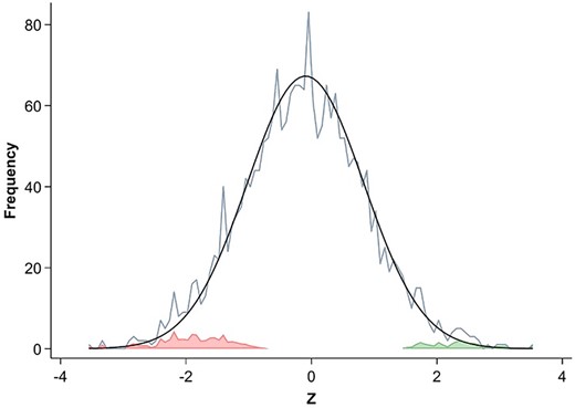
Finite mixture analysis of association Z‐score distribution. The smooth black curve is an estimate of the hypothetical normal distribution of null associations, based on the observed range and density of Z‐scores near zero. The jagged light‐blue line shows the distribution (in bins of 1/14–0.0714 Z‐score units) of all actual, observed Z‐scores of the taxa‐skeletal measure associations. The colored areas represent the number of taxa‐skeletal measure associations not expected to occur within the hypothetical normal distribution of null effects, and thus representing potentially true associations: red the number of potentially true negative effects, and green the potentially true positive effects. The false discovery rates at each location on the Z scale can be visually estimated by comparing the height of the red or green areas at that location to the height of the overall histogram (light‐blue line) at the same location. See Supplemental Statistical Methods for a fuller description of the finite mixture model.
In studies of the association of microbiome composition with skeletal traits, low expected false discovery rate (eg, FDR < 0.1) for promisingly large associations would be desirable. The Z‐scores observed among the most robust associations in the current studies had estimated log2 fold changes of approximately 0.25 per standard deviation of bone measure (Table 2), with standard errors on the order of 0.1. An optimistic power calculation assuming enrichment fraction and effect sizes at similar levels to what was observed in the current study estimates that a sample size of no less than n = 6000 would be required, and upward of n = 10,000 or more may be required if the true effect sizes are smaller, the enrichment fraction is lower, or both.
Discussion
The gut microbiome has been linked to bone homeostasis in a variety of animal experiments, and probiotic supplements have been reported to have beneficial effects on bone density in postmenopausal women,(20) but there are few data concerning what elements of the microbiome might be related to skeletal health in humans. This is the first large study to test for associations between the microbiome and skeletal measures in humans. We found suggestive evidence that the abundances of several bacterial genera were associated with skeletal bone density, microarchitecture, and strength. Four genera were associated with at least one skeletal measure (Anaerofilum, Methanomassiliicoccus, Ruminiclostridium 9, and Tyzzerella). Two more (Lactobacillus and Streptococcus) were associated using somewhat less stringent significance criteria. Most associations were negative, but others suggested higher genera abundance was associated with indices of better skeletal health. This is concordant with dysbiotic shifts in other health conditions, which are frequently not attributable to single organisms, but which can instead modify any one of several “more” or “less beneficial” microbes among different individuals. Moreover, these relationships were generally consistent across a variety of skeletal measurement sites. Although the study must be considered exploratory and we cannot be highly confident of the associations we identified, our results should be useful in highlighting specific bacterial genera and pathways that may be of particular interest for additional confirmatory research. The genera we report as having the most robust associations have not, to our knowledge, been previously reported to affect skeletal traits and the mechanisms that might mediate those effects are unknown. More detailed studies using metagenomic data generated by shotgun sequencing (ie, at the species or functional level) would be better suited to identify biological functions that might be important for bone.
The patterns of the associations of the microbiome with skeletal measures may also be informative. The associations between genera abundance and bone were generally consistent across multiple measurement sites and bone compartments. For instance, genera most strongly associated with lower trabecular BMD were also likely to be associated with lower cortical thickness and higher cortical porosity, and hence lower integral BMD and failure load. This pattern is expected if mediated by a broad‐based effect of the microbiome on remodeling balance (either positive or negative) that would drive density and porosity measures in opposite directions. This also suggests that putative influences of microbial composition on bone were not limited to a particular bone compartment but involve widespread remodeling‐based mechanisms. To some extent, these consistent associations across measures of several anatomical sites are expected based on underlying correlations among the skeletal measures (Supplemental Fig. 1). However, these are sometimes quite weak in isolation (eg, r ~ 0.4), making it difficult to assume they completely explain the consistent associations of microbes with multiple skeletal measures. The associations with distal radial cortical porosity were somewhat less consistent, but the accuracy of cortical porosity measures at the distal radius is questionable. Overall, the consistency and biological plausibility of the patterns of associations argues against statistical artifact, and suggests an underlying microbiome‐bone interaction.
A notable finding given the nontrivial size of our sample of participants (n > 800) was that there were few strong associations between taxa and skeletal measures. This is again in some ways to be expected, as the routes by which the gut microbiome can affect systemic physiology are relatively narrow. Molecular mechanisms to transmit chemical products or immune activity from the gut throughout the body for bone development and/or maintenance must of necessity act gradually at best, and in extreme cases the latter will be confounded with overt inflammatory disease. A further challenge in this cohort of older men is that variation in the HRpQCT features also reflects genetic variation and the influence of lifetime exposure to environmental effects. Thus, some of the effects of the microbiome would likely be proportionately small. Our experience with these data suggests that studies similar to this one would have to be large (≥6000 participants) to provide adequate power to confidently detect meaningful associations. Cohort studies that utilize metagenomic data with resolution exceeding that of our 16S rRNA gene amplicon sequencing might need even greater population sizes to provide sufficient power. These challenges are similar to studies using genetic markers, in which effect sizes of common variants with phenotypes are of extremely small magnitude.(64‐66) Conversely, studies of more focused patient populations might require fewer numbers. For instance, studies of participants with specific clinical characteristics or studies that exclude variables that might confound the relationships,(67) could improve power.
The study had several strengths. MrOS is a well‐phenotyped cohort with extensive information about the participants' clinical characteristics. We excluded men with recent exposure to antibiotics, and adjusted for potentially confounding factors. Fecal samples were collected using an approach known to preserve nucleic acids and well‐established methods were used for bacterial genotyping and analyses. Standardized bone measures were performed at several skeletal sites using state‐of‐the‐art approaches.
We also identified several important limitations. Most importantly, our strongest associations between bone phenotypes and the gut microbiome were relatively small, and it is clear that even in >800 men these results must be considered exploratory. On the other hand, the genera that we have identified may be very useful as specific targets for future replication studies, especially if adequately powered, and eventually to identify pathways or to design targeted research using mouse models. While the homogeneity of the MrOS aids in analysis, this was as a result a cross sectional evaluation that included only elderly males; we could not evaluate the potential influence of age, sex, or racial/ethnic differences, longitudinal measures of the gut microbiome and the skeleton, and their interrelationships. On the other hand, although the human microbiome can vary in response to a variety of stimuli, it is generally relatively self‐stable over long periods.(68,69) Also, as is often necessary in human populations, the study was observational, and causation cannot be determined from our results. Finally, although we examined multivariable models that included a number of factors that might influence bone, the microbiome or their interactions, there may be additional confounding variables that were not considered.
In summary, we examined associations of genus‐level gut microbial components with measures of bone density, microarchitecture, and strength in a cohort of older men. We found several taxa that were nominally associated with bone measures, and a compelling pattern of genus‐bone relationships that suggest the influences of microbial composition on bone are not limited to a particular bone compartment but involve more generalized mechanisms. The magnitudes of the associations we detected were not large, but therapeutically targeting the microbiome over many years could still translate into preservation or enhancement of skeletal integrity. Clearly, additional studies should involve larger cohorts of men and women over wider age ranges and/or more causally incisive methods.
Acknowledgments
The Osteoporotic Fractures in Men (MrOS) Study was supported by the National Institute on Aging; the National Institute of Arthritis and Musculoskeletal and Skin Diseases; the National Center for Advancing Translational Sciences; the National Institutes of Health Roadmap for Medical Research (grant numbers U01 AG027810, U01 AG042124, U01 AG042139, U01 AG042140, U01 AG042143, U01 AG042145, U01 AG042168, U01 AR066160, and UL1 TR000128). DPK’s effort and a portion of gut microbiome genotyping were supported by the National Institute of Arthritis and Musculoskeletal and Skin Diseases R01 AR061445. We acknowledge the essential contributions of all the MrOS participants, investigators and staff whose dedication, commitment, and contributions make the MrOS study possible.
Authors’ roles: EO contributed to data collection, study conceptualization, drafting of the analysis plan, data curation, formal analysis, interpretation of results, writing of the original and final draft of the manuscript, and supervision of the study. NP contributed to analysis and reviewing of the manuscript. JW contributed to analysis, interpretation of results, and reviewing of the manuscript. JL contributed to data curation, interpretation of results, and writing and reviewing of the manuscript. NN contributed to interpretation of results and reviewing of the manuscript. JEW contributed to the design of the analysis plan, interpretation of results, and reviewing of the manuscript. CH contributed to the design of the analysis plan, interpretation of results, and reviewing of the manuscript. LL contributed to interpretation of results and reviewing of the manuscript. DPK contributed to data collection, study conceptualization, interpretation of results, reviewing of the manuscript, and supervision of the study.
Conflicts of Interest
EO: Consultation for Amgen, Bayer, BioCon, Radius; research support from Mereo; travel funding from the OI Foundation. DPK has received grants to his institution from Amgen, Inc, and Radius Health; he has received consulting fees from Solarea Bio and Pfizer for serving on Scientific Advisory Boards, and royalties for publication in UpToDate by Wolters Kluwer. NP, JW, JL, NN, JEW, CH, and LL have nothing to declare.
Peer Review
The peer review history for this article is available at https://publons.com/publon/10.1002/jbmr.4518.
Data Availability Statement
The data that support the findings of this study are available upon request. In addition, MrOS data, including the microbiome genotypes, are available at MrOS Online (https://mrosonline.ucsf.edu/).
References
Author notes
[Correction added on 4 March 2022, after first online publication: Author Contribution section has been removed]
